An Optimized HT-Based Method for the Analysis of Inter-Area Oscillations on Electrical Systems

Abstract

The paper deals with a novel method to measure inter-area oscillations, i.e., electromechanical oscillations involving groups of generators geographically distant from one another and ranging within the frequency interval from 0.1 Hz up to 1 Hz. The estimation of the parameters characterizing inter-area oscillations is a crucial objective in order to take the necessary actions to avoid the instability of the transmission electrical system. The proposed approach is a signal-based method, which uses samples of electrical signals acquired by the phasor measurement unit (PMU) and processes them to extract the individual oscillations and, for each of them, determine their characteristic parameters such as frequency and damping. The method is based on Hilbert transformations, but it is optimized through further algorithms aiming at (i) improving the ability to separate different oscillatory components, even at frequencies very close to each other, (ii) enhancing the accuracy associated with the damping estimates of each oscillation, and (iii) increasing the robustness to the noise affecting the acquired signal. Results obtained in the presence of signals involving the composition of two oscillations, whose damping and frequency have been varied, are presented. Tests were conducted with signals either synthesized in simulated experiment or generated and acquired with actual laboratory instrumentation.

1. Introduction

Inter-area oscillations are phenomena that affect electricity systems interconnecting areas geographically distant from each other, such as different nations. Various phenomena can cause the inter-area oscillation; a rapid change of load, a line faults, the control and regulation necessary to guarantee the stability of large power system area, the connection between large power system with weak lines. Practically, all these phenomena determine a transient in the transferred power which bring the system into a new balance operating condition [1].

The balance point will be reached after a redefinition of the power contributions of the various generators connected to the system [2].

The dynamic modes characterizing the motion from a balance condition to another belong to the Low Frequency Oscillations (LFOs) category. In particular, each i-th mode of evolution of the electrical system is typically representable according to the following expression:

$$y_i\left(t\right)=A_i{e}^{-d_{i}t}sin\left(2\pi f_{i}t+{\phi }_i\right),$$

(1)

where $A_i$ is the amplitude, $d_i$ is the damping coefficient, $f_i$ is the frequency and ${\phi }_i$ is the starting phase.

Usually, the frequency range is from 0.1 Hz up to 2 Hz and the oscillations are divided into two categories:

-

inter-area oscillations from 0.1 to 1 Hz;

-

local oscillations from 1 up to 2 Hz.

As regards the damping value, a generic classification adopted in the scientific literature is the following [3,4,5]:

• damped $d_i\in \left[0.05,+\infty \right[$;
• weakly damped $d_i\in \left]0,0.05\right[$;
• divergent $d_i\in \left]-\infty ,0\right[$.

The accurate estimate of the damping coefficient of the oscillations is a fundamental issue. In fact, particularly dangerous for the stability of the electrical system are the oscillations that exhibit a weakly positive or negative damping coefficient. In fact, if the oscillations are not attenuated for a long time or they are amplified and can reach dangerous amplitudes, they can cause the intervention of protections or, in the worst cases, could jeopardize network operation.

The estimation of damping coefficient is crucial to take the adequate countermeasures in order to assure the network stability. On the other hand, the inter-area oscillations are often characterized by weak damping, and the estimation of the damping sign is not a straightforward process.

In the paper, a novel method based on an optimized combination between the Hilbert transform (HT) and non-linear least square (NLS) fitting is proposed. The method aims at separating the dynamic modes that are combined in the acquired signal and estimating frequency and damping coefficient of the individual oscillations.

The paper is organized as follows. In Section 2 the main methods described in the literature for the analysis of inter-area oscillations are discussed. In Section 3 theoretical fundamentals about HT are given. In Section 4 the proposed approach is presented. The results obtained from both numerical and experimental assessment are reported in Section 5. Section 6 deals with the digital signal processing method to analyze oscillations characterized by very close frequency values. Concluding remarks are given in Section 7.

2. Approaches Available In Literature

Recognizing as soon as possible the divergent or weakly damped oscillations is a fundamental task to be able of employing appropriate countermeasures and consequently guarantee the stability of the electrical systems. The estimation algorithm has to exhibit, as main characteristics, a low computational burden, high robustness to noise, high accuracy in parameter estimation and no need of a priori information about the signal of interest.

Generally, the methodologies reported in scientific literature follow two different approaches [6]:

• Model-based;
• Signal-based.

As reported in [6,7,8] the model-based approach aims at estimating the parameters of synchronous generators in order to derive an overall model of the electrical system. The possibility of retrieving the system model is appealing, but these methods are characterized by high computational burden. The order of the equivalent model, in fact, can be very high, since it is strictly dependent on the extension of the electrical system [9]. Moreover, the obtained equivalent model is valid for a limited time interval because of the constant evolution of the network topology.

Although many methods have been proposed aiming at power system reduction for dynamic analysis with consequent lower computational burden, the results obtained do not seem to be sufficiently accurate.

An interesting approach is represented by a hybrid method based on the Kalman Filter, reported in [10,11], that combines the model-based and signal-based methodologies. This method processes signals acquired through the phasor measurement units (PMUs) to obtain the overall model of the electrical system. As known, the Kalman filter is a valuable approach for real-time signal analysis, thanks to its adaptive behavior. However, also this method exhibits a significant computational burden, because of the matrices dimensions, dependent on the complexity of the model. For this reason, this approach is usually adopted to estimate damping coefficient and frequency of the dominant mode, with consequent loss of information about eventual other oscillatory modes. Moreover, the proper initial choice of the measurement noise covariance and process noise covariance is the most sensitive issue characterizing the Kalman filter.

Owing to the analytical difficulties involved in Model-based approach, the scientific literature is increasingly oriented towards the study and development of a Signal-based method for the analysis of LFOs.

The typical structure of such algorithms is characterized by two steps: decomposition in mono-component signals, and estimation of signal parameters.

Several solutions available in the literature match with this type of approach: variational mode decomposition (VMD) and Teager–Kaiser in [12]; discrete Fourier transform (DFT) and curve-fitting in frequency domain in [13]; singular value decomposition (SVD) and matrix pencil method in [14]; empirical mode decomposition (EMD) and Hilbert spectrum analysis in [15,16], as an example. Each of the mentioned algorithms is characterized by different advantages and drawbacks. Generally, the most critical issue is related to the non-stationary and non-linear nature of the electrical system [17].

The most analyzed approach, in the literature, is undoubtedly the Prony method [3]. The Prony algorithm is a parametric method of direct signal decomposition. It assumes that the acquired signal can be approximated by a sum of damped sinusoids. This method does not need a priori information, since a precise model has been chosen to fit the signal; moreover it only needs to analyze a period and a half of the oscillations in order to estimate its damping and frequency. However, as is well known in the literature, the algorithm is very sensitive to the noise, so that in some cases additional mono-component signals are not detected. The direct consequence is a limited accuracy in the estimation of the parameters of interest. In order to solve this problem, pre-filtering techniques are used for noise cancellation, such as digital filters and EMD, causing an increase of the computational burden of the algorithm.

In [18] the authors propose an improved Prony method where the method is coupled with a low order model of the signal and the parameters are evaluated with a least square method. Instead, the paper [19] introduces a covariance matrix in order to improve the estimation of low frequencies with Prony method.

Another interesting approach involves the use of multivariate autoregressive model which helps in the identification of low frequencies signals. In [20] the identification of inter-area oscillations is carried out through the use of Yule–Walker estimator; the results highlight the good performance of the algorithm also when the measurement noise and the lost of packets affects the signal.

Authors have finally focused their attention on Hilbert-based approaches as in [21,22]. These methods are flexible, do not require information about the signal and are suitable for representing non-linear and non-stationary systems. The critical issue is the process for separating the mono-component oscillations; even a small edge effect causes a considerable lack of accuracy in the damping estimate.

3. Ht Fundamentals

The HT of a real signal $x\left(t\right)$ is defined as the following convolution integral:

$$H\left[x\left(t\right)\right]=\frac{1}{\pi }P.V.{\int }_{+\infty }^{-\infty }\frac{x\left(\tau \right)}{t-\tau }d\tau ,$$

(2)

where it is necessary to consider the Cauchy Principal Value ($P.V.$) of the integral, resulting from the eventual singularity of the integrand function.

The HT has the fundamental property of shifting the phase of the real signal of a positive angle equal to $\frac{\pi }{2}$, without the need of changing the representation domain (both HT input and output belong to the time domain). This characteristic is useful to obtain the analytic signal of a real signal $x\left(t\right)$.

$$z\left(t\right)=x\left(t\right)+j{x}_H\left(t\right)=x\left(t\right)+jH\left[x\left(t\right)\right]$$

(3)

The signal can be written according to the polar coordinates, so it can be seen as the product between two terms: the first one takes into account the amplitude modulation and the second one includes the phase modulation. If the signal exhibits slow amplitude variations with respect to the phase variations, i.e., if the amplitude modulation is characterized by frequencies much lower then those characterizing the phase modulation [23], the analytic signal in polar coordinates can be considered as a rotating phasor:

$$z\left(t\right)=A\left(t\right)e^{j\theta \left(t\right)}.$$

(4)

The time-varying amplitude is the envelope of the real signal and phase can be estimated according to the equations:

$$\begin{array}{ccc}\hfill A\left(t\right)& =& \sqrt{x{\left(t\right)}^2+H{\left[x\left(t\right)\right]}^2}\hfill \end{array}$$

(5)

$$\begin{array}{ccc}\hfill \theta \left(t\right)& =& arctan\frac{H\left[x\left(t\right)\right]}{x\left(t\right)}.\hfill \end{array}$$

(6)

From the expression of the instantaneous phase it is possible to determine the instantaneous frequency, defined as:

$$f\left(t\right)=\frac{1}{2\pi }\frac{d{\theta }_u\left(t\right)}{dt},{\theta }_u\left(t\right)=\theta \left(t\right)+\Lambda \left(t\right),$$

(7)

where $\Lambda \left(t\right)$ is a function whose values are integer multiples of $\pi$, required to assure the continuity of the phase ${\theta }_u\left(t\right)$.

If $x\left(t\right)$ is a damped oscillation, the HT is a suitable tool for estimating the oscillation parameters. Equation (7), in fact, provides the oscillation frequency; the instantaneous amplitude, instead, provides the damping factor. In fact, the instantaneous amplitude can be written as:

$$A\left(t\right)=A_1{e}^{-\sigma t}$$

(8)

where $A_1$ is the starting amplitude and $\sigma$ is the damping coefficient. By performing the natural logarithm:

$$ln\left[A\left(t\right)\right]=ln\left(A_1\right)-\sigma t$$

(9)

The damping coefficient, thus, can be evaluated performing the time derivative of the terms of Equation (9):

$$\sigma =\frac{d}{dt}\left(\sigma t\right)=-\frac{d}{dt}\left[ln\left(A\left(t\right)\right)\right].$$

(10)

Since HT is a linear operation, the following equation holds:

$$H\left[kx\left(t\right)\right]=kH\left[x\left(t\right)\right]$$

(11)

where k is a generic constant.

By keeping this in mind and by recalling the property of shifting the phase, if $x\left(t\right)$ is a cosinusoidal function, according to Equation (11), its HT is:

$$H\left[Acos\left(\omega t+\phi \right)\right]=Asin\left(\omega t+\phi \right),$$

(12)

where A is the constant amplitude, $\omega$ stands for the angular frequency, $\phi$ represents the phase and $sin\left(\omega t+\phi \right)$ is the HT of the cosine. This relationship will be exploited in the successive section.

Lastly, if $x\left(t\right)$ is the product of two functions, namely f and g, the HT of $x\left(t\right)$ could be evaluated as the multiplication between $f\left(t\right)$ and the HT of $g\left(t\right)$, according to:

$$H\left[f\left(t\right)·g\left(t\right)\right]=f\left(t\right)·H\left[g\left(t\right)\right].$$

(13)

This equivalence is maintained if f and g satisfy the Bedrosian’s conditions [16,21], i.e., if their spectra are separated and f is characterized by low-frequency components with respect to g.

4. Proposed Approach

The proposed method is event-based, i.e., the algorithm has to run when an oscillation is detected, in order to estimate its parameters; in normal operating conditions, the results of the parameters estimation would be unmeaningful.

The proposed approach consists of three main steps:

• Separation of individual oscillations: the acquired signal is processed in order to recognize the individual inter-area oscillations;
• Oscillations reshaping: the estimation of each component is refined by matching a damped oscillation model;
• Correction of Gibbs effect and parameter estimation: the estimate of the full signal is further refined in order to remove Gibbs oscillations and to evaluate the frequency and damping coefficients of the oscillations.

In the following subsections these steps are described in detail.

4.1. Separation of Individual Oscillations

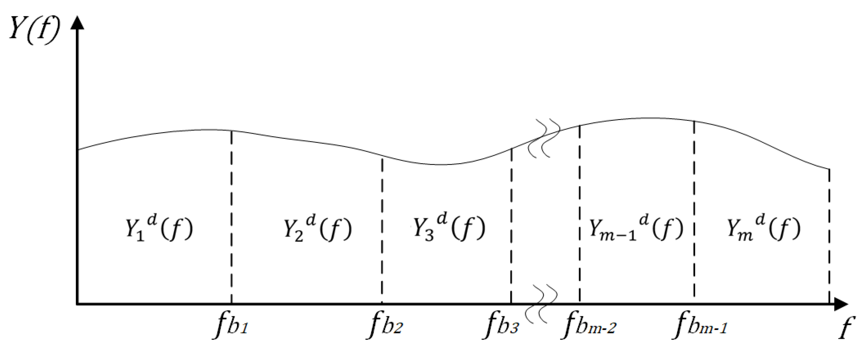
The Hilbert-based algorithm uses a decomposition method, presented and demonstrated in [21]. According to the theorem stated in [21], it is possible to describe the signal acquired by the PMU $y\left(t\right)$ as the sum of m components $y_i^d\left(t\right)$:

$$\sum _{i=1}^m{y}_i^d\left(t\right).$$

(14)

The components $y_i^d$, with i ranging from 1 to m, are such that their spectra $Y_i^d\left(f\right)$ are not overlapped and are significant only in a narrow frequency band, as show in Figure 1, delimited by the frequencies $f_{b_{i-1}}$ and $f_{b_i}$ (with $f_{b_0}=0$), in the following referred to as bisecting frequencies; moreover, the sum of all the spectra $Y_i^d\left(f\right)$ is equal to the spectrum $Y\left(f\right)$ of the signal $y\left(t\right)$.

If $s_i\left(t\right)$ is the time domain signal corresponding to the portion of the spectrum $Y\left(f\right)$ of Figure 1 between the frequencies 0 and $f_{b_i}$, each of the components $y_i^d$ can be obtained by subtraction according to the following formulas:

$$y_i^d\left(t\right)=s_i\left(t\right)-s_{i-1}\left(t\right),$$

(15)

where, if i is equal to 1, then $s_{i-1}\left(t\right)=s_0\left(t\right)=0$ and if i is equal to m, then $s_m\left(t\right)=y\left(t\right)$.

The terms $s_i\left(t\right)$ are evaluated, as demonstrated in [21] according to the Bedrosian theorem:

$$s_i\left(t\right)=sin\left(2\pi f_{b_i}t\right)H\left[y\left(t\right)cos\left(2\pi f_{b_i}t\right)\right]-cos\left(2\pi f_{b_i}t\right)H\left[y\left(t\right)sin\left(2\pi f_{b_i}t\right)\right]$$

(16)

It is worth noting that the truncation of the spectra in Figure 1 generates oscillations on the estimated signal $s_i\left(t\right)$, well known as Gibbs effect. At this aim, in Equation (12) authors preferred the use of Hilbert-Boche transform [24] that is able to reduce this undesired phenomenon.

The authors applied this method to extract the individual oscillations from the signal acquired by a PMU. It should be noted that, in this case, the spectra of the mono-components are overlapped, because the presence of damping causes the spread of the spectrum. The estimated components $y_i^d$ therefore do not exactly fit the oscillations composing the input signal. In other words, the portion $Y_i^d$ of the spectrum results from the super-position of two components. Therefore, the separation algorithm will return a $y_i^d$ component that differs from the mono-component oscillation; the more overlapping the spectra of the component oscillations, the higher the estimation error.

In [21] the LP-periodogram is used to identify the number of components and the values $f_{b_i}$ of the bisecting frequencies that delimit the spectrum intervals. The number of oscillations is given by the peaks of the spectrum, whereas the value of $f_{b_i}$ is calculated as the arithmetic average of the frequencies corresponding to the periodogram peak.

If the signal of interest $y\left(t\right)$ can be modeled as a sum of damped oscillations, each of them is characterized by a narrow band spectrum. Thus, the presented separation method can be exploited in order to obtain the individual oscillations.

The component signals $y_i^d$ therefore, are the inter-area oscillations affecting the bus voltages, whose frequency and damping coefficients have to be estimated.

The separation is applicable if a bisecting frequency can be recognized. Thus the proposed method requires the detection of at least two peaks in the spectrum. If only one peak is visible, because the acquired signal involves only one oscillation or because it involves oscillations whose frequency distance is lower than the spectral resolution, the method fails.

Also the presence of undesired frequency components, not related to inter-area oscillation, could put in crisis the separation method. In the paper, however, authors have taken into account only canonical signals observed in power system; the robustness to other type of components is going to be studied in future works.

Optimal Choice of Bisecting Frequencies

As aforementioned, in order to separate the oscillations, the bisecting frequency is typically evaluated as the average between the frequencies of two sequential peaks of the periodogram of the input signal [21]. Actually, the optimal separation does not correspond to this frequency. For the sake of clarity, a signal obtained by the sum of two damped oscillations is taken into account. In particular, the signal is described by the following analytical expression:

$$y\left(t\right)=30e^{-0.3t}sin\left(\pi t\right)+5e^{-0.1t}sin\left(1.6\pi t\right).$$

(17)

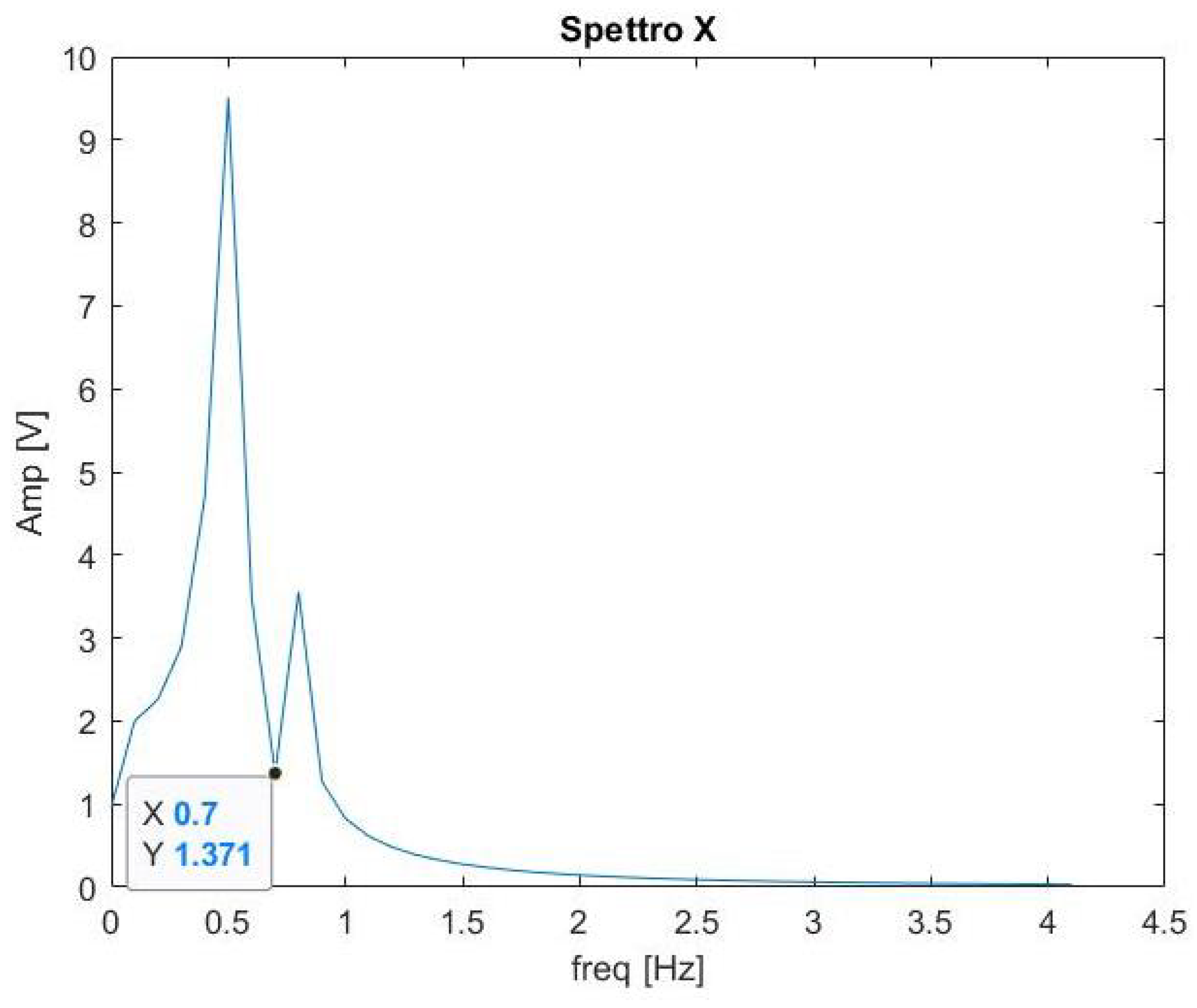
The spectrum of this signal, shown in Figure 2 exhibits only two peaks centered at the frequencies 0.8 Hz and 0.5 Hz. The bisecting frequency, evaluated as average frequency, is equal to:

$$f_b=\frac{f_1+f_2}{2}=\frac{0.8+0.5}{2}=0.65\mathrm{Hz}$$

(18)

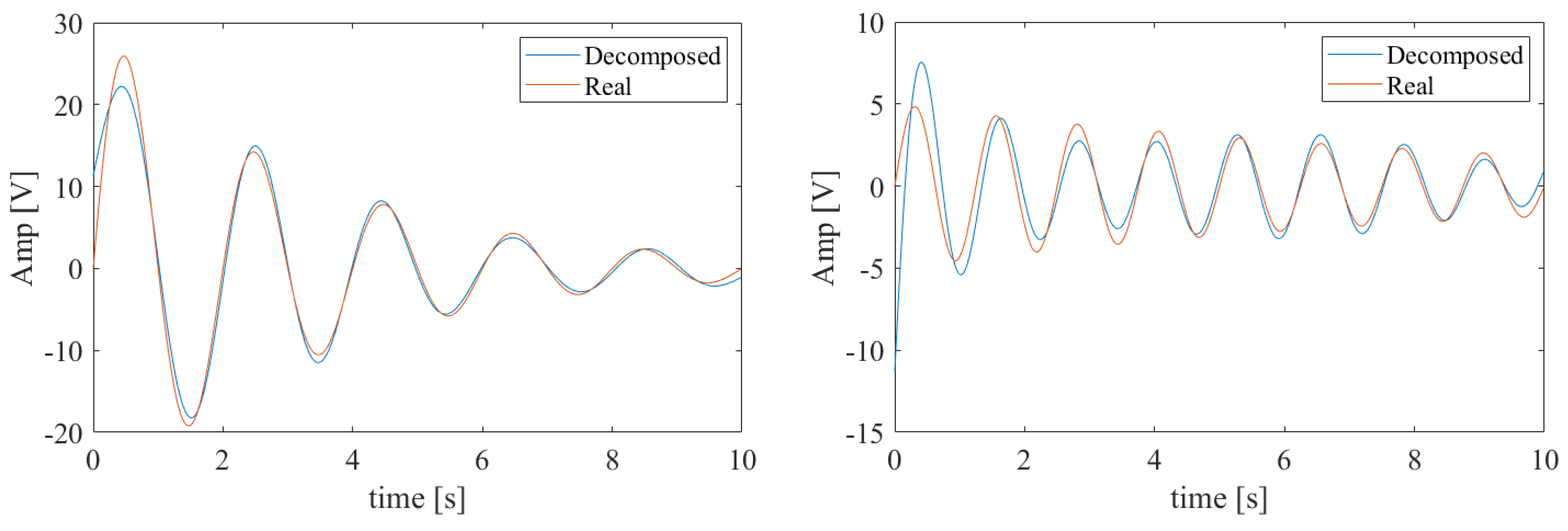
The separation algorithm, described in the previous section, performed with $f_b$, provides two components, whose time evolution, compared with that of the nominal oscillations, is shown in Figure 3.

Besides an amplitude error caused by the Gibbs effect, it can be noted that even the zero crossing of the estimated components do not coincide with the oscillations composing the input signal.

This means that the estimation of the frequency of the two mono-component signals suffers from a slight deviation from the actual value.

The authors, therefore, decided to improve the criterion for choosing the bisecting frequency. In particular, the frequency corresponding to the minimum of the portion of the signal spectrum delimited by two peaks is selected as the bisecting frequency.

In this way, in fact, the separation error is minimized when the spectra of the two components are partially overlapped.

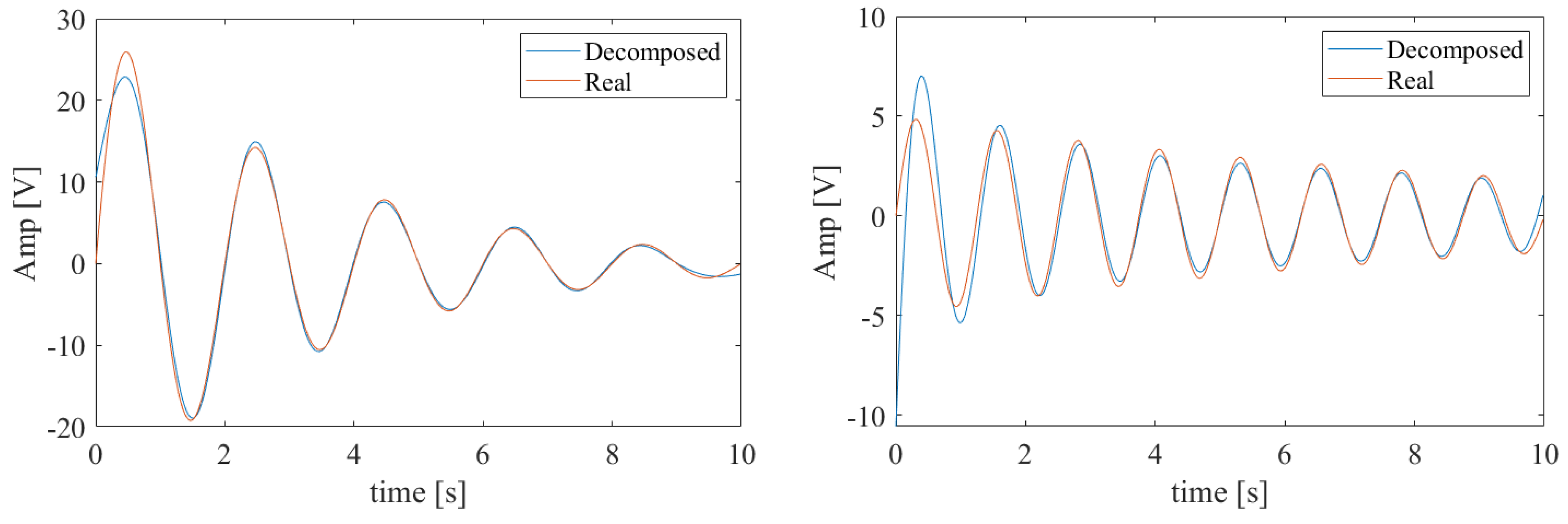
As it can be appreciated from the spectrum of Figure 2, the estimated bisecting frequency, in this case, is equal to 0.7 Hz; the corresponding mono-component signals obtained by the separation algorithm are shown in Figure 4. It should be noted that, although the Gibbs effect is still present, the estimated oscillations match the frequency values characterizing the nominal input signals.

4.2. Oscillations Reshaping

Despite of the adoption of some optimizations such as the Hilbert–Boche method and better choice of sectioning frequency, a deviation between the actual components and their estimates, due both to Gibbs effect and overlapping oscillations spectra, is still significantly appreciable. As noticeable in Figure 4, the estimate suffers from a distortion mainly evident at the oscillation edges, that hugely affects the damping estimate.

The second step of the proposed approach, then, relies on the reshaping of the mono-component signals. In detail, for each component, a non-linear least squares (NLS) regression algorithm is performed in order to detect the damped oscillation that is the best fit of the estimated mono-component.

At this aim the optimization tools of MATLAB^® (R2018B, MathWorks, Natick, MA, USA) has been exploited [22], where the sequential quadratic programming (SQP) [25] has been set as minimization method and the fitting function is given by the formula:

$$y_i^{dr}\left(t\right)=A_i{e}^{d_{i}t}sin\left(2\pi f_{i}t+{\phi }_i\right),$$

(19)

where the unknown variables are the amplitude $A_i$, the damping coefficient $d_i$, the frequency $f_i$ and the starting phase ${\phi }_i$; $y_i^{dr}\left(t\right)$ is the reshaped version of each estimated mono-component $y_i^d\left(t\right)$. Figure 5 shows the obtained oscillations after the reshaping performed on the mono-components of Figure 4. It can be noted that, for both the oscillations, the edge effects have been substantially reduced and the estimated frequencies almost match the actual ones. However, a slight amplitude deviation is still appreciable and, therefore, the oscillations estimate has to be further adjusted in order to properly estimate the damping coefficients.

The reshaped components are used as initial estimate for the successive step, that aims at accurately estimating the amplitude of the components and, consequently, the damping coefficient.

4.3. Correction of Gibbs Effect and Parameters Estimation

Finally, the third step of the proposed approach consists of a further non-linear regression.

This time, the processed signal is the estimate of the overall signal $y_i^r\left(t\right)$, obtained by summing all the reshaped oscillations $y_i^{dr}\left(t\right)$.

Also this regression is an NLS, performed by exploiting the SQP method. However, the fitting function is given by:

$$\widehat{y}\left(t\right)=\sum _{i=1}^m{A}_i{e}^{d_{i}t}sin\left(2\pi f_{i}t+{\phi }_i\right)$$

(20)

All the amplitudes, frequencies, damping coefficients and starting phases are the unknown variables. It should, however, be pointed out that the NLS algorithm converges rapidly (typically a time of less than 100 ms is required) since the initial values of the variables are those obtained from the second step and, therefore, already quite close to the values of the final fitting solution. Moreover, the NLS algorithm allows us to set the constraints (frequency and damping can vary in definite ranges) that limit the range of the possible solutions and favor the convergence.

In order to highlight the improvements introduced by the double regression algorithm,

Table 1. Variable estimates after the third step of the proposed method.

	Component 1
	Actual	Estimated
Damping [s${}^{-1}$]	0.3	0.29999
Frequency [Hz]	0.5	0.49999
Amplitude [V]	30	29.99999
	Component 2
	Actual	Estimated
Damping [s${}^{-1}$]	0.1	0.09999
Frequency [Hz]	0.8	0.79999
Amplitude [V]	5	4.99999

shows the actual parameters and those estimated after the third step of the proposed method, for the components of the example signal described by equation Equation (17).

5. Experimental Assessment

The proposed method has been assessed through both numerical and emulated experiments.

A preliminary design of the tests was required in order to set: (i) the duration of the signal time window to be analyzed; (ii) the sampling frequency characterizing the acquired signal, (iii) the characteristics of the test signal, and (iv) the figure of merit (FoM) to be used to evaluate the method performance.

The duration of the time window has been chosen in order to both minimize the response time of the algorithm and acquire at least one cycle of each mono-component signal (required condition for assuring the convergence of the NLS algorithm). The inter-area oscillations are characterized by a frequency range from 0.1 Hz up to 1 Hz; the window, assuring one cycle of a 0.1 Hz oscillation, is characterized by the width of 10 s.

As regards the sampling frequency, it has been selected according to the frequencies recommended for PMUs by Standard [26]. A minimum value of 5 S/s is mandatory to comply with the Nyquist–Shannon sampling theorem. However, low sampling rates correspond to few numbers of points acquired in each oscillation period, making unreliable the result of the NLS algorithms. On the other hand, higher sampling frequencies would result in increased number of points to be processed, and, consequently, higher computational burden and response time. A trade-off sampling frequency equal to 50 S/s has been selected. This sampling rate presents another advantage: being nominally equal to the fundamental frequency of the bus voltage, if the sampling operation is perfectly synchronized with the fundamental frequency, only the contribution of low frequency components is visible in the acquired signal.

The considered test signal is composed by two inter-area oscillations and is expressed by the formula:

$$y\left(t\right)=1e^{-d_{1}t}sin\left(2\pi f_{1}t\right)+1e^{-d_{2}t}sin\left(2\pi f_{2}t\right).$$

(21)

For the sake of simplicity, the amplitudes of both the oscillations have been set equal to 1 V and the starting phases has been set equal to zero. The frequency and the damping coefficient of the oscillations have been varied within their typical intervals reported in literature [1].

In particular, two sets of experiments have been planned. In the first one, referred in the following to as Test I, the frequencies $f_1$ and $f_2$ of the two oscillations have been set equal to 0.1 Hz and 0.6 Hz respectively. The damping coefficients, instead, are varied within the following intervals:

• $d_1=[-0.05,0.3]$s${}^{-1}$;
• $d_2=[-0.05,0.3]$s${}^{-1}$.

In the second set of experiments, referred in the following to as Test II, the damping coefficients have been set equal to 0.1 and 0.3 s${}^{-1}$, respectively, and the frequencies have been varied in order to change the frequency distance between the oscillations. In particular, an experiment has been performed by setting $f_1=0.1$ Hz and varying $f_2$ from 1 Hz to 0.3 Hz; another experiment has been carried out by setting $f_2$ equal to 1 Hz and varying $f_1$ from 0.1 to 0.8 Hz. This way, Thanks to the variation of the distance $|f_1-f_2|$ between the frequencies of the two components, it has been possible to assess method performance in the case of components characterized by low (near 0.1 Hz) or high (near 1 Hz) oscillation frequency.

The selected FoM is the deviation between estimated $\widehat{d}$ and nominal d damping coefficients for both the oscillations:

$$\Delta d=\widehat{d}-d$$

(22)

Particular attention, in fact, has been paid to the ability of the method to correctly estimate the oscillations damping coefficient, that is the parameter that mostly predicts potential system instability [27,28].

5.1. Numerical Tests with Ideal Signal

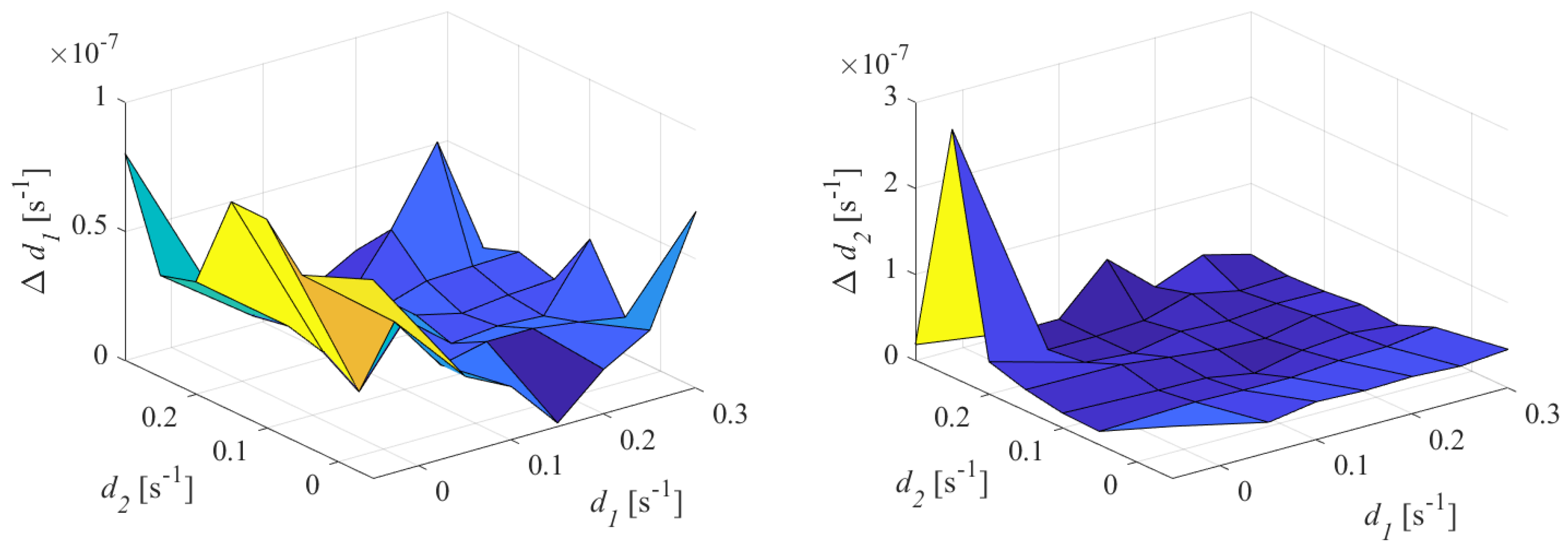
The preliminary performance assessment of the proposed approach has been carried out through numerical tests in MATLAB^® environment; to this aim, the signal of Equation (21) has been synthesized as input, according to the selected sampling rate of 50 S/s. The evolution of estimated values of FoMs versus the damping coefficients of the two mono-components for Test I is shown in Figure 6.

The proposed method exhibits excellent performance regardless the damping coefficients characterizing the oscillations. In fact, it is able to recognize and separate the two oscillations composing the test signal and, for both the components, it is able to estimate the damping coefficient with a $\Delta d$ values lower than ${10}^{-7}$s${}^{-1}$ (corresponding to a relative percentage deviation of ${10}^{-4}$%).

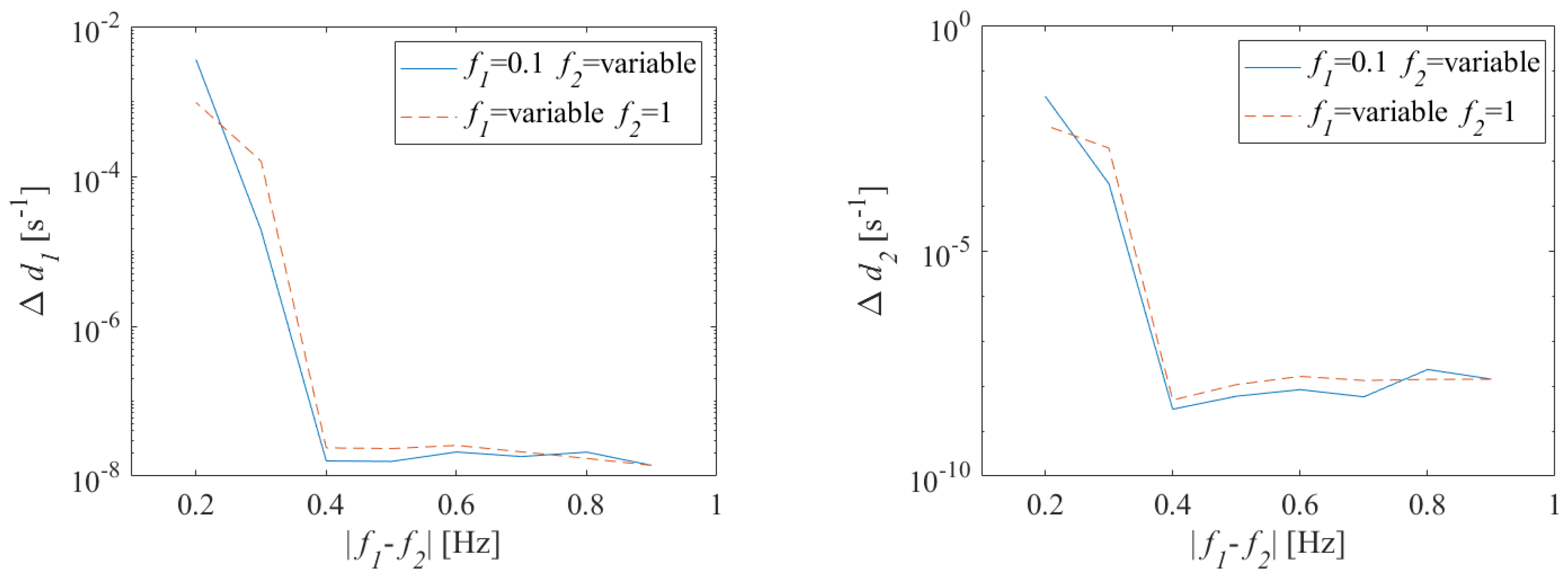
The results obtained in test II conditions are shown in Figure 7. To better appreciate method performance, the logarithmic scale has been set for the vertical axis of both graphs.

For both damping coefficients, estimate deviation $\Delta d$ was lower than ${10}^{-7}$s${}^{-1}$ as long as the oscillation frequency distance was at least 0.4 Hz, corresponding to four times the spectral resolution associated with the sampling conditions. When $|f_1-f_2|$ was reduced, an increase in the estimate deviation was experienced; however, when $|f_1-f_2|$ is equal to 0.2 Hz, the estimated $\Delta d$ was lower than ${10}^{-2}$s${}^{-1}$ for both the oscillations. This result was expected, since when the frequency are nearer, the spectra of the two mono-components are more overlapped and the distortion resulting from the separation procedure increases. A particular case consists of two oscillations whose frequency distance $|f_1-f_2|$ was lower than 0.2 Hz; the method described in Section 4 failed, because the two oscillations were so near in frequency that a minimum in the signal spectrum is not detected and a bisecting frequency cannot be estimated. To obtain a suitable damping estimate even in such critical conditions, the measurement method has been improved by means of a further digital signal processing procedure that will be described in detail in Section 6.

Finally, $\Delta d$ turns out to be sensitive to the frequency distance between the two oscillations, but, given the same $|f_1-f_2|$, the estimate of damping coefficients seemed not to sense if the oscillations were located at either high or low frequency.

5.2. Numerical Test with Noise and Quantization

Successive tests have been performed in conditions more similar to the actual sampling conditions. Thus, the effects of both noise and the quantization resulting from the analog to digital conversion stage have been added to the test signal of Equation (21).

The signal has been corrupted with white noise, whose amplitude has been set in order to assure a Signal to Noise Ratio (SNR) equal to 40 dB.

The use of an eight-bit analog-to-digital converter (ADC) has been hypothesized for introducing the quantization.

Since the presence of noise causes an inevitable dispersion of the algorithm results, the authors preferred to carry out N equal to 50 repeated trials, for each frequency and damping condition. The damping estimates of the 50 tests were processed in order to evaluate the mean value and associated standard deviation. The FoM evaluated in these tests were the mean and the standard deviation of the measured $\Delta d_i$, with i = 1, 2, …, N:

$$\mu \left(\Delta d\right)=\frac{1}{N}\sum _{i=1}^N\left(\Delta d_i\right)$$

(23)

$$\sigma \left(\Delta d\right)=\sqrt{\frac{1}{N-1}\sum _{i=1}^N{\left(\Delta d_i\right)}^2}.$$

(24)

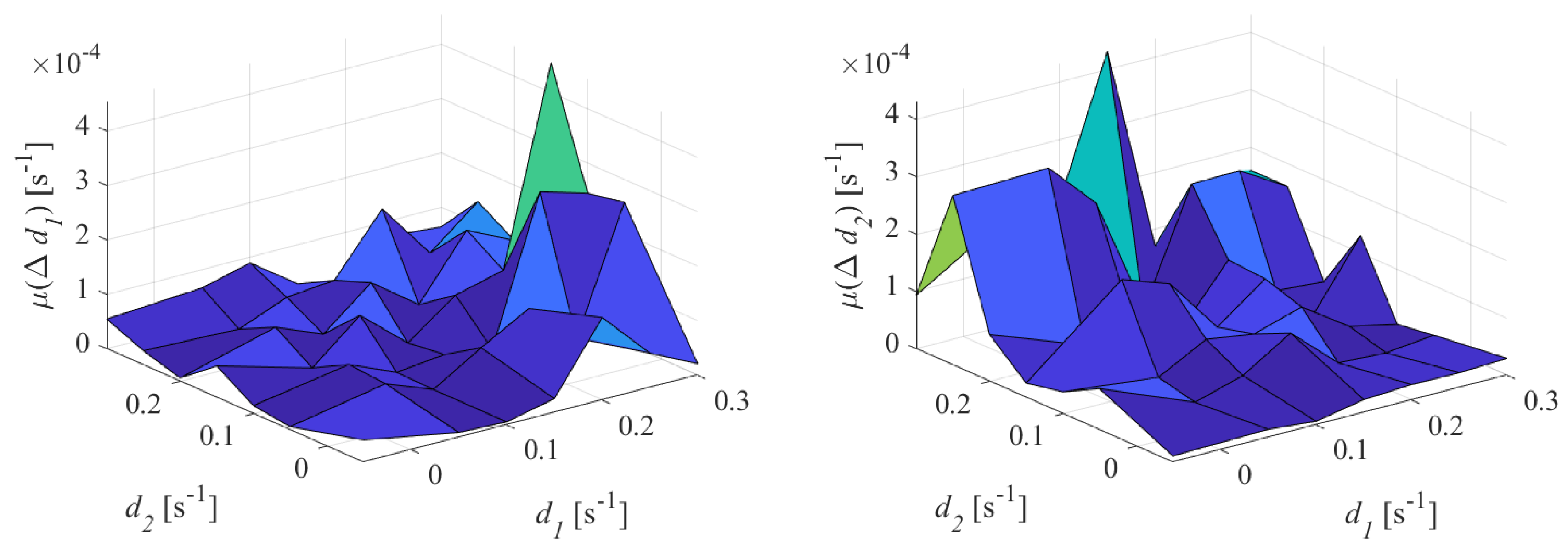
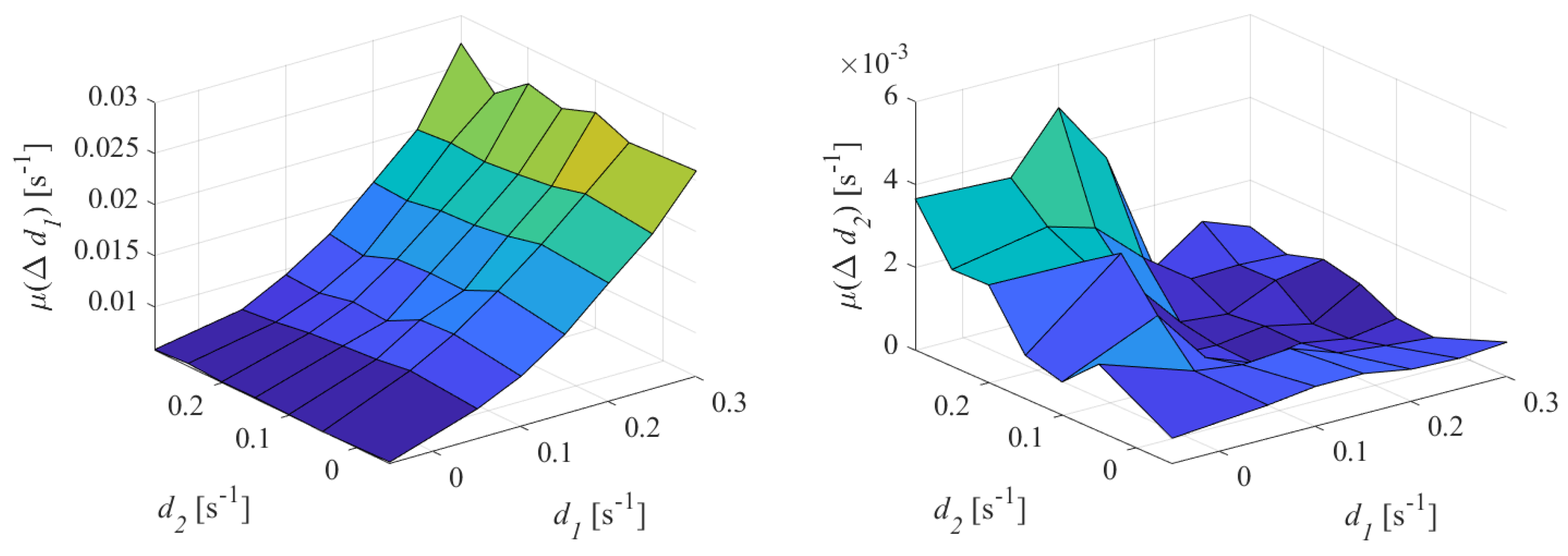
Figure 8 shows the evolution of the estimated FoM versus damping coefficient, for both the oscillation in Test I configuration.

With respect to the values observed with ideal signals, an increase of estimate $\Delta d$ for both damping coefficients was appreciated. For both oscillations, however, the deviation of the estimate remained lower than ${10}^{-4}$s${}^{-1}$.

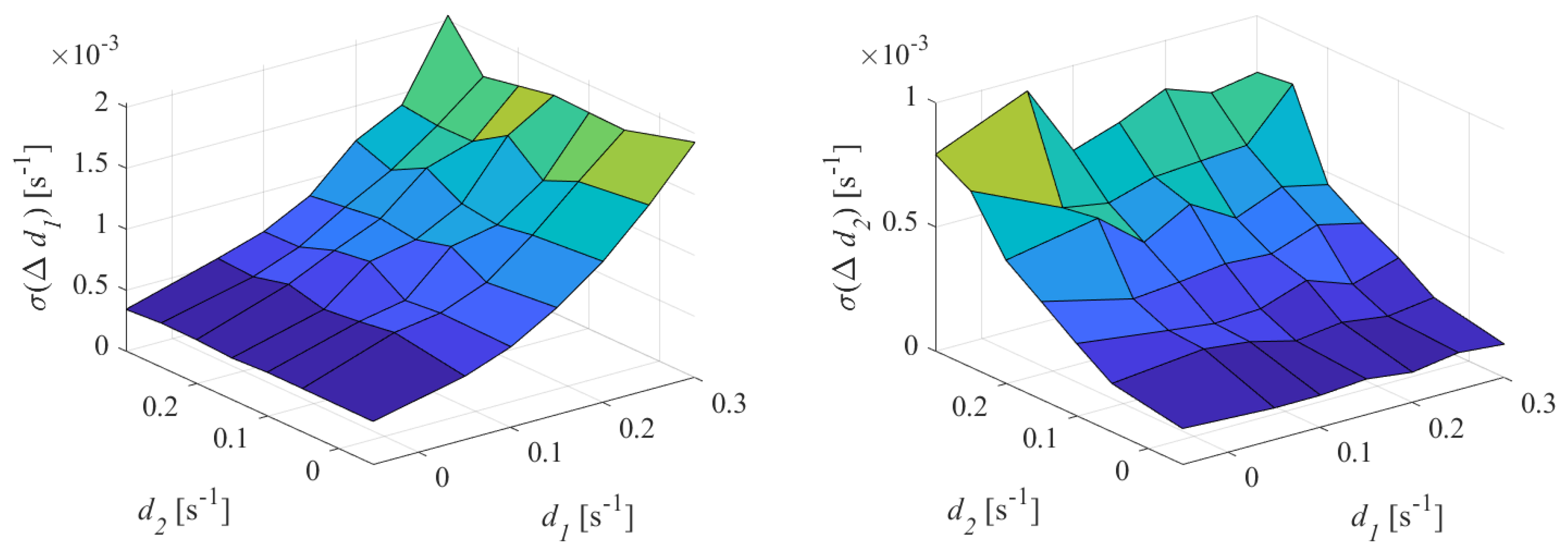
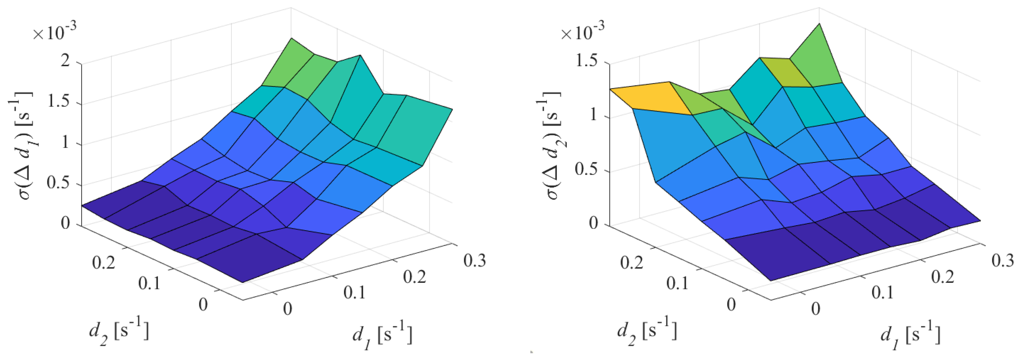
The standard deviations associated with the estimates of the damping coefficients are shown in Figure 9.

From the graph of the standard deviation associated with the damping estimates of the first oscillation, it can be noted that $\sigma (\Delta d_1)$ assumed values lower than 0.3 × 10${}^{-3}$s${}^{-1}$ when the first oscillation was weakly damped. The higher the damping $d_1$, the higher the standard deviation, which reached up to about 2 × 10${}^{-3}$s${}^{-1}$. The evolution of $\sigma (\Delta d_1)$ seemed to be independent on the values of $d_2$.

A similar behavior was observed on the damping estimates of the second oscillation: the standard deviation increased, up to 1.3 × 10${}^{-3}$s${}^{-1}$, as the damping coefficient of the second oscillation rose, while it was not affected by the values of the damping coefficient of the first oscillation.

It has to be noted that oscillations characterized by high damping coefficient are not dangerous for the system stability, therefore the behavior of the proposed method with respect to noise can be tolerated.

It can be concluded that the proposed algorithm was sensitive to the noise affecting the input signal and the sensitivity coefficient depends on the value of the damping coefficients. The noise, in particular, did not affect the mean of the damping estimates, but impacts directly on the dispersion of the results.

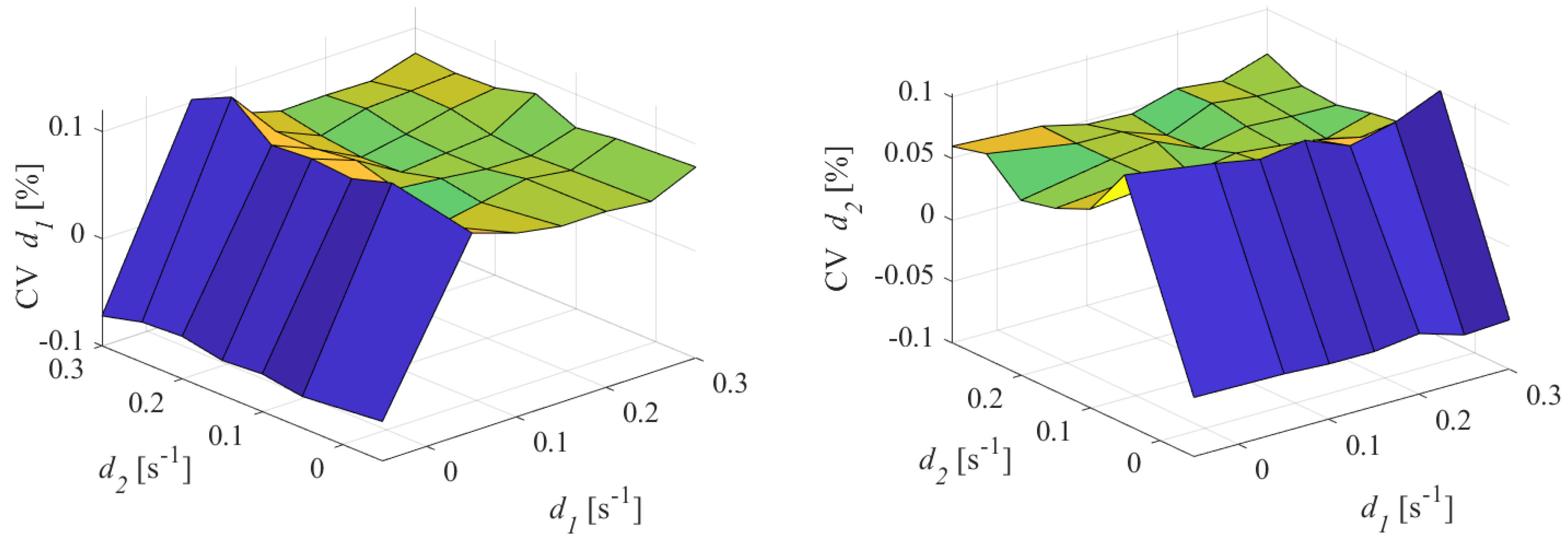
For the sake of clarity, the coefficient of variation (CV), proposed in [29] has also been evaluated. It is defined as:

$$CV=100·\frac{{\sigma }_{\overline{d_i}}}{\overline{d_i}},$$

(25)

where $\overline{d_i}$ is the mean value of the estimated $d_i$ and ${\sigma }_{\overline{d_i}}$ is the standard deviation of the mean. The obtained results are shown in Figure 10.

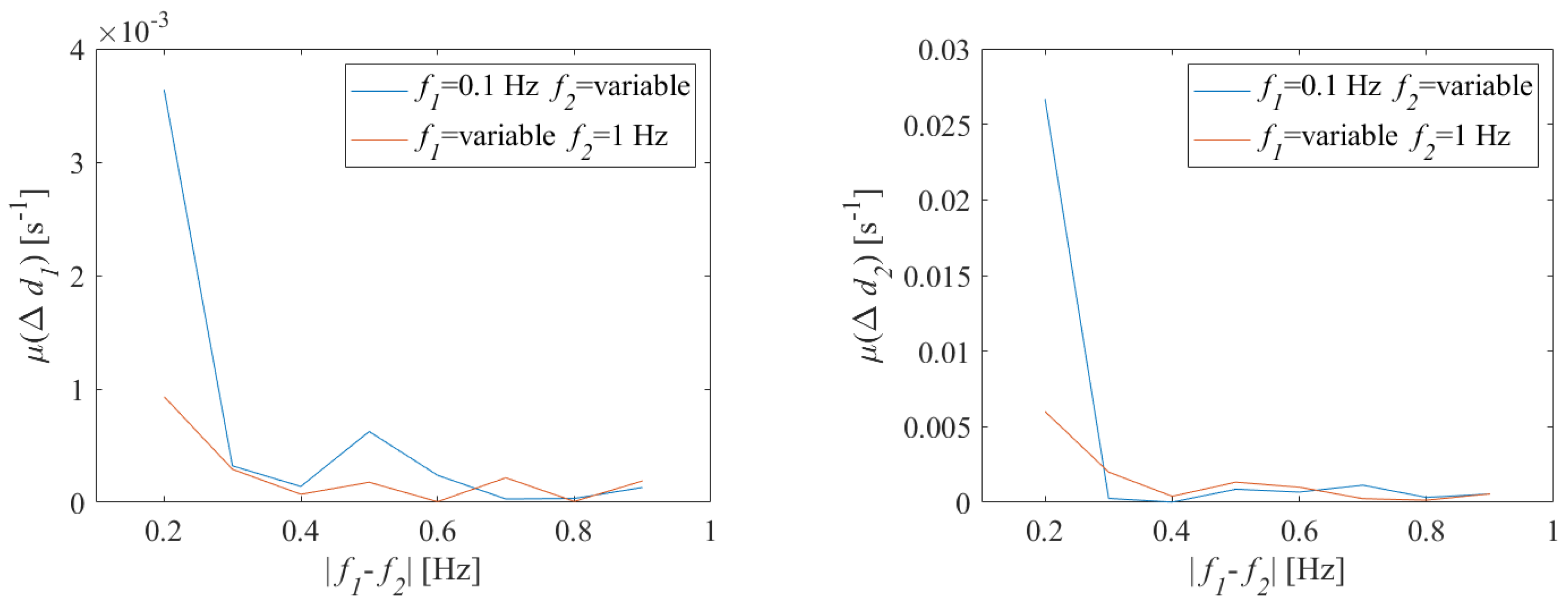
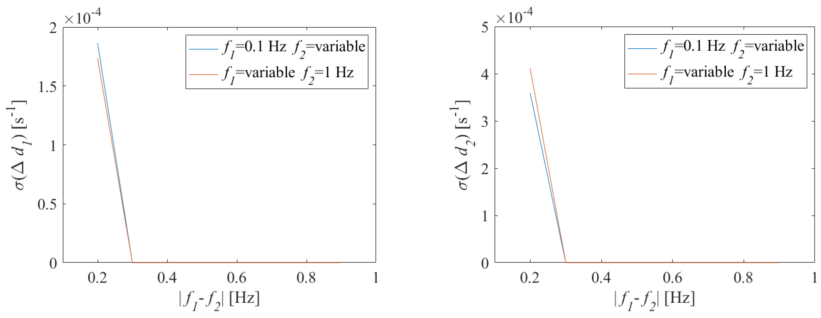
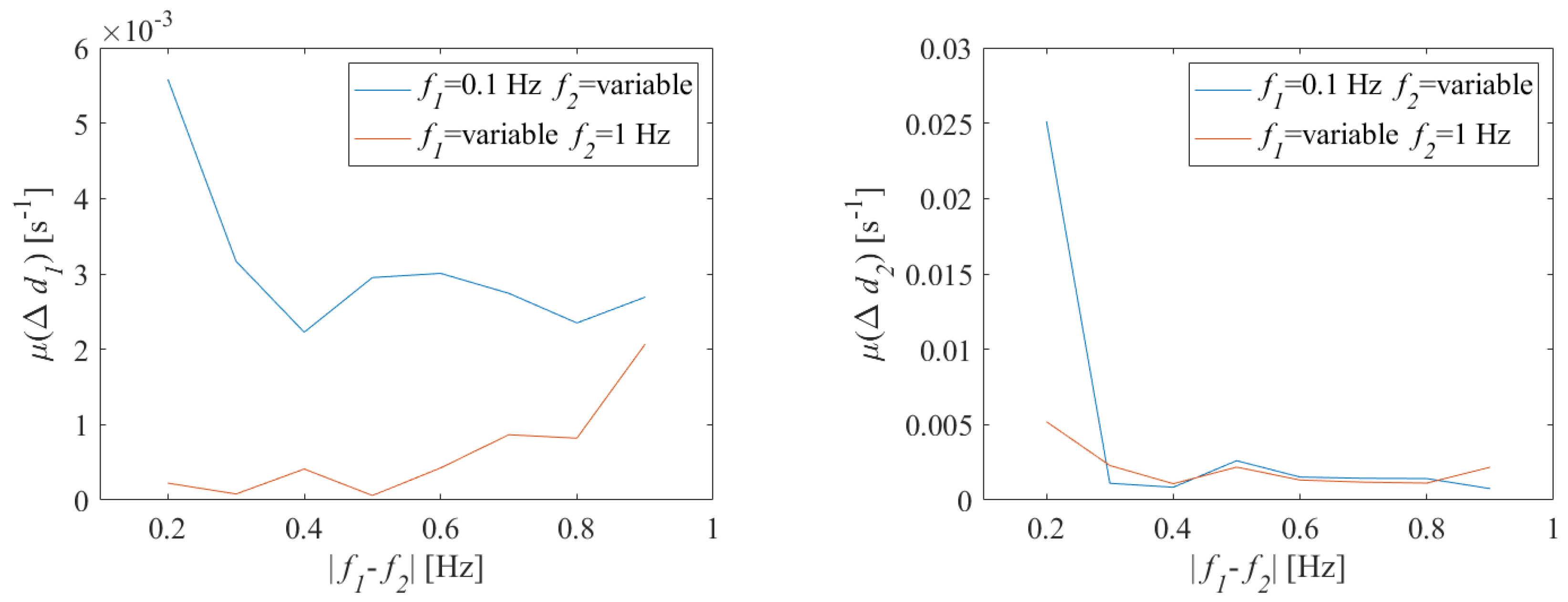
The absolute value of CV is always lower than 0.1%. The lower the damping coefficient $d_1$, the higher the CV; moreover, the CV of $d_1$ was not dependent on the values of $d_2$. Similar behavior can be observed for the CV of $d_2$. The results obtained from the experiments conducted according to Test II configuration are shown in Figure 11.

As long as $|f_1-f_2|$ was higher than 0.3 Hz, measure $\Delta d$ was lower than ${10}^{-3}$s${}^{-1}$ for the first oscillation and lower than ${10}^{-2}$s${}^{-1}$ for the second oscillation. When $|f_1-f_2|$ is 0.2 Hz, the estimate deviation increased for both damping coefficients as expected. The corresponding standard deviations are reported in Figure 12. As noticeable, the noise presence influenced the dispersion of the estimates of damping coefficient only when $|f_1-f_2|$ is 0.2 Hz and, however, the standard deviation was lower than ${10}^{-3}$s${}^{-1}$.

5.3. Test Conducted on Digitized Signals

Finally, further tests have been performed on signals, emulating the composition of two oscillations, generated and acquired through real laboratory instrumentation.

To carry out the experimental tests, a laboratory test bench has been set up consisting of:

• Arbitrary waveform generator Agilent 33220A,
• Eight-bit digital oscilloscope Tektronix TDS 210,
• National Instruments GPIB-USB-HS interface.

A proper software has been developed in the National Instruments LabVIEW^TM environment, in order to (i) synthesize the test signal according to Equation (21) in dependence on the desired frequencies and damping coefficients; (ii) transfer the waveform to the memory of the waveform generator, (iii) gather the samples acquired by the digital oscilloscope, and (iv) apply the proposed method to estimate the damping coefficients.

Again, 50 repeated measurements have been performed for each combination of damping coefficients and both the mean values and the standard deviations have been evaluated.

The mean of the deviation between the damping estimates and the nominal values is shown, for both oscillations, in Figure 13.

It is evident that, in this case, the deviation of the damping estimates are characterized by values higher than those observed in numerical tests.

Moreover it can be noted that the deviation of the estimates exhibits a trend sensitive to the damping coefficients; in particular, the damping estimates worsen as the damping coefficient increases.

The evaluated standard deviations are shown in Figure 14.

In this case, the trend and values of the standard deviation associated with the damping estimates is similar to those observed in numerical tests in the presence of noise and quantization presented in Section 5.2. The dispersion of the estimation results, therefore, is related exclusively to the presence of noise; the transition from numerical signals affected by a Gaussian noise to actually generated signals did not change the performance of the method, in terms of dispersion of measurement results.

The results obtained in Test II configuration shown in Figure 15.

Also in this case, it can be noted that the deviation of the mean value of the damping coefficient estimates has increased by about 10 times. For the sake of brevity the plots of the standard deviations and CV are not reported; however, values comparable with those observed in Section 5.2 have been appreciated.

It is worth noting that further tests have been carried out with oscillations characterized by different amplitude and with signal acquired through non-coherent sampling conditions. For the sake of brevity the graphs are not reported. However, the obtained results proved that also in these tests, the performance of the method are similar to the reported in this Section 5.2.

5.4. Test Conducted on Inter-Area Oscillations Provided by Simulated Systems

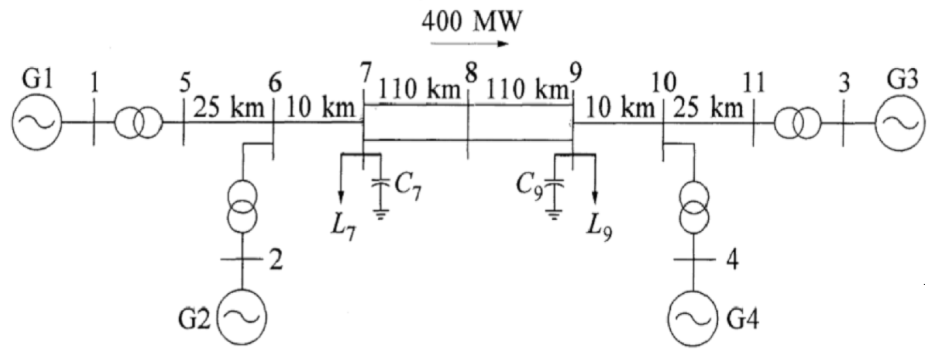
In order to assess the method with a signal as similar as possible to a signal acquired during an inter-area oscillation, the Kundur’s four-machine two-area test system [30], whose single line diagram is shown in Figure 16, has been adopted.

The Kundur’s model has been implemented in Simulink^® (Simulink 9.2, MathWorks, Natick, MA, USA); a PMU to measure the bus voltage has been placed near the generator G2 and a three-phase fault has been simulated, in order to obtain the test signal. The voltage acquired by the PMU is nominally the combination of a local oscillation (the oscillation of G1 with respect to G2) and an inter-area oscillation (the oscillation of the area including G3 and G4 with respect to that including G1 and G2).

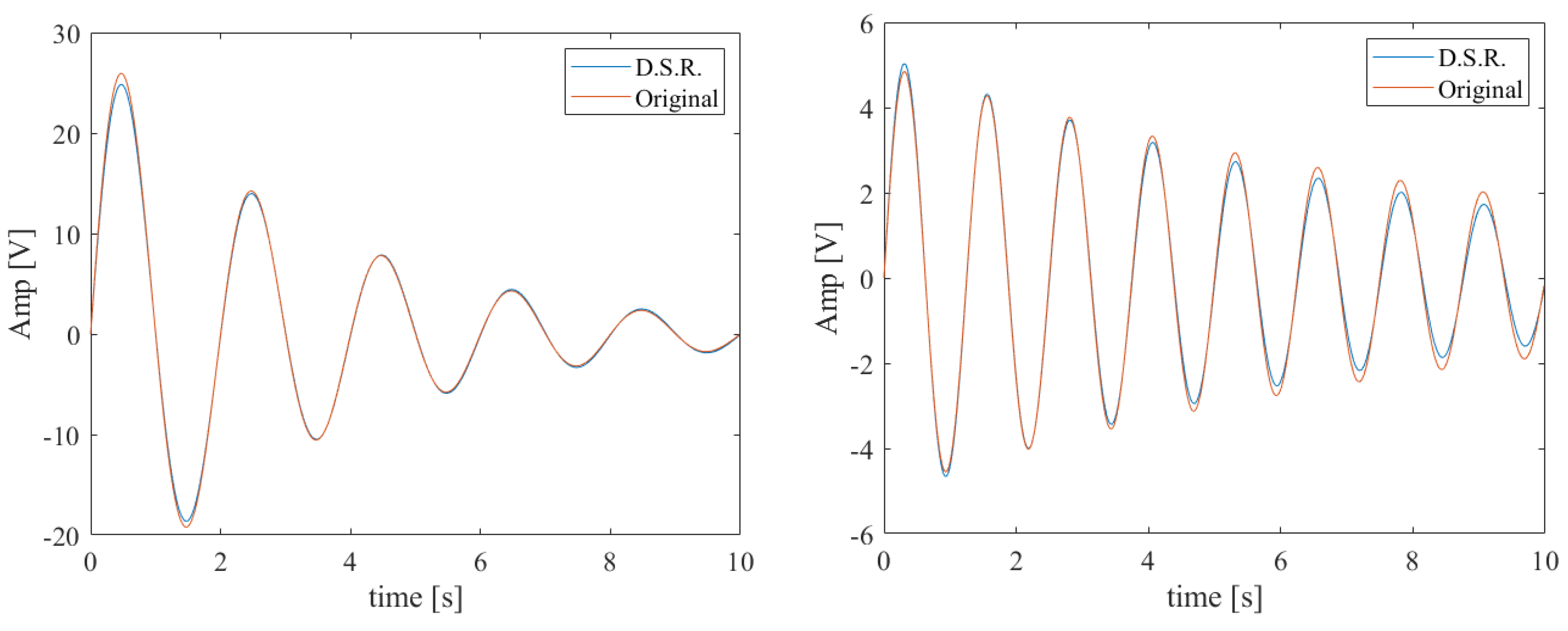
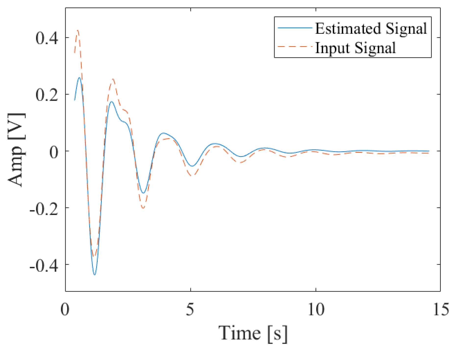
The initial part of the signal acquired by the PMU has been cut to remove the fault transient; the obtained signal, versus time, is shown in Figure 17, represented with the red dashed line.

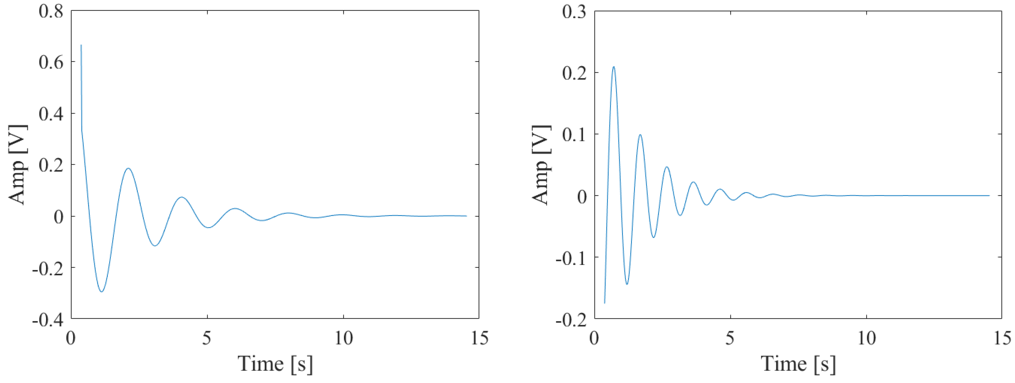
The test signal has been processed according to the proposed approach. Two oscillations have been detected; in fact, the spectrum of the signal exhibited two peaks at the frequencies of 0.53 Hz (compatible with an inter-area oscillation) and 1.1 Hz (compatible with a local oscillation), respectively. The monocomponents estimated by the proposed method are shown in Figure 18.

In particular, the estimated parameters are reported in

Table 2. Estimates of oscillations parameters of Kundir’s model.

Component	Frequency	Damping
Component 1	0.532 [Hz]	0.475 [s${}^{-1}$]
Component 2	1.121 [Hz]	0.767 [s${}^{-1}$]

.

In order to evaluate the quality of the separation method, the two obtained monocomponents have been summed and the resulting signal, shown in Figure 17 and referred to as estimated signal, has been compared with the input test signal. It can be observed that the estimated signal accurately fits the time evolution of test signal.

6. Processing for Near Frequency Oscillations

As mentioned above, the proposed separation method fails if the oscillations are characterized by frequencies that are distant less than twice the spectral resolution.

The authors have improved the method, providing specific processing for this case, which is recognized because only one peak is detected in the spectrum.

In particular, the developed algorithm examines, by means of an NLS regression in the time domain, the signal acquired by the PMU through a moving time window; the algorithm stops when the root mean square (RMS) deviation between the input signal and the best fit is lower than a fixed threshold.

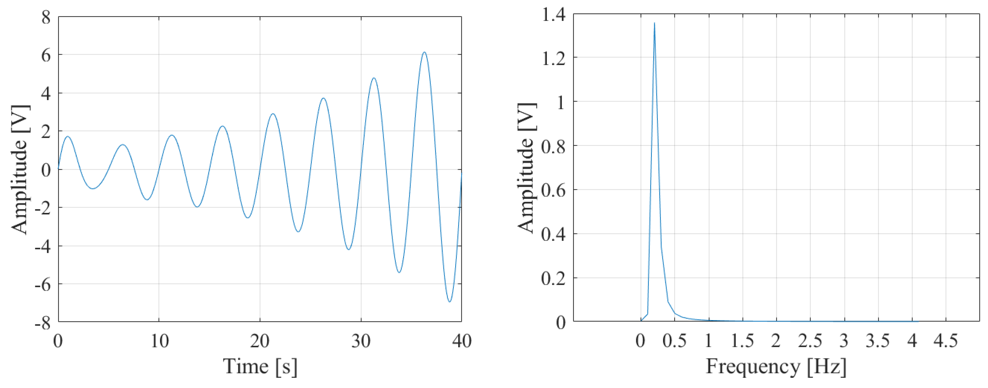
For the sake of clarity, the signal described by the following formula is considered:

$$y\left(t\right)=1e^{0.05t}sin\left(0.4\pi t\right)+1e^{-0.3t}sin\left(0.6\pi t\right).$$

(26)

The test signal consists of the sum of two oscillations, the first one divergent and the second one damped, characterized by frequencies equal to 0.2 Hz and 0.3 Hz, respectively. Both the time evolution and the spectrum of the test signal are shown in Figure 19.

It has to be observed that the spectrum of Figure 19 can also be associated to a single tone component, that has been acquired with non-coherent sampling conditions; so the separation of this signal in two oscillations could lead to unmeaningful information. For this reason, the algorithm search for the best mono-component oscillation that fits the input signal.

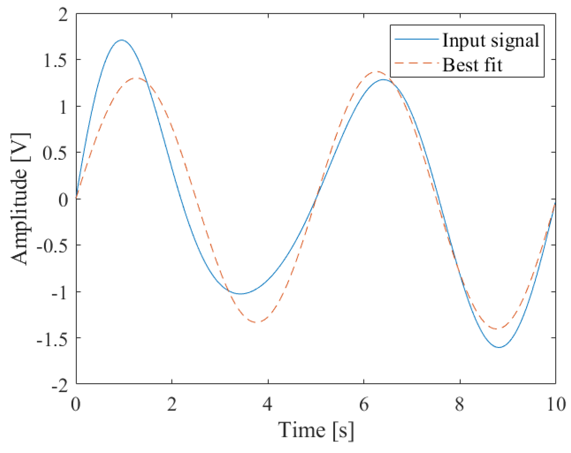
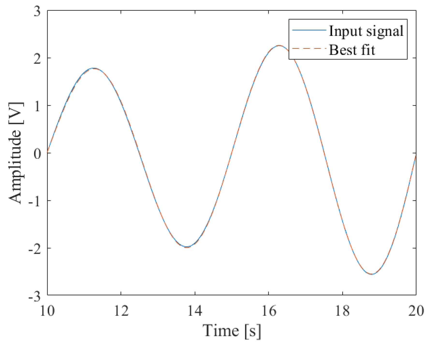
A 10 s time window of the test signal is shown in Figure 20. The samples of this window are given as input to an NLS minimization that fits the test signal with a single damped oscillation. If the actual signal is compared with the obtained best fit, it can be noted that the deviation in the estimate is high. The estimate of the damping coefficient is shown in the second column of

Table 3. Estimates of the damping coefficient.

Actual	Estimate on First Window	Estimate on Second Window
−0.05 [s${}^{-1}$]	−0.0103 [s${}^{-1}$]	−0.0496 [s${}^{-1}$]

.

This result is expected because, in the first 10 s, the analyzed signal is actually the combination of two oscillations, while the algorithm tries to fit the signal with only one oscillatory mono-component.

It should be noted, however, that although the NLS regression provides a rough estimate, it provides a negative sign of the damping. Therefore the regression is able to identify the presence of a divergent oscillation. This result can be exploited to raise an alert situation: the damping coefficient is not known accurately, but there is a divergent oscillation to keep under control.

The next step in the algorithm is to examine the successive 10 s window and repeat the nonlinear regression. Both the signal and the best fit are shown in Figure 21. It can be noted that, this time, the best fit had a time evolution similar to that of the input signal. Damped oscillations, in fact, have been attenuated and the test signal is suitably approximable by a mono-component signal.

The estimated damping is reported in the third column of Table 3.

The algorithm stops when the root mean square error (RMSE) between the samples of the acquired signal and those of the best fit is lower than a set threshold.

Summarizing, in the case of frequencies very close to each other, the proposed algorithm estimated a single damping, as if it detected only one oscillation. Various numerical tests have been performed, in different conditions, in order to verify the behavior of the algorithm. In the case of divergent oscillations, the algorithm is always capable of recognizing them since the estimated damping results negative in the first 10 s time window. Successively, as the time window moves, the algorithm refines the damping estimate.

Further tests have been carried out with signal involving only damped oscillations, also characterized by amplitudes quite different one from each other. In the first window, the algorithm can be strongly influenced by the component characterized by the highest amplitude; in this case the RMSE value can be very small, since the NLS result properly fits the acquired signal. The setting of the proper RMSE threshold, then, is a fundamental issue to assure the reliability of the method. A threshold equal to 0.1% of the amplitude has proved to be optimal in all the experiments.

It can be concluded that:

• if the signal contains a divergent oscillation, the estimated damping is the negative one, since the divergent oscillation exhibits a larger amplitude that masks the damped oscillations in the NLS minimization.
• if the signal contains only damped oscillations, the estimated damping coefficient is the one characterized by the smallest absolute value, i.e., that associated with the most persistent oscillation; therefore the algorithm is also able to recognize weakly damped oscillations.

7. Conclusions

In the paper a novel algorithm for the analysis and parameters estimation of inter-area oscillations has been proposed. The method consists of three steps: (i) the separation, according to an optimal bisection frequency, of the input signal in individual mono-component oscillations; (ii) reshaping of each mono-component in order to minimize the distortion due to the separation; (iii) correction of Gibbs effect and parameters estimation through a NLS algorithm.

Several tests, both with numerical and experimental signals have been carried out in order to assess the method. With respect to solutions already available in literature, the proposed method is characterized by excellent performance in terms of accuracy of the parameter estimates and robustness to noise.

As regards the computational burden and the response time, the proposed method allows to acquire and process a reduced number of samples, in favor of the computational resources. In particular, the described results have been obtained by processing 500 samples acquired with a sampling rate of 50 S/s. Concerning the response time, the time required by the algorithm execution is negligible with respect to the time spent for the acquisition of the signal samples. The method performance, in fact, is sensitive to the spectral resolution and, then, to the size of the analyzed time window. By considering the typical values of frequency and damping coefficient characterizing the inter-area oscillations, the authors have selected, as optimal trade off between the spectral resolution and the response time, a time window of 10 s.

The ongoing activity is focused on the development of a dedicated measurement instrument. At this aim, the realized algorithm has to be converted from MATLAB^® and transferred on an embedded system.