Diesel Mean Value Engine Modeling Based on Thermodynamic Cycle Simulation Using Artificial Neural Network

Abstract

This study aims to construct a reduced thermodynamic cycle model with high accuracy and high model execution speed based on artificial neural network training for real-time numerical analysis. This paper proposes a method of constructing a fast average-value model by combining a 1D plant model and exhaust gas recirculation (EGR) control logic. The combustion model of the detailed model uses a direct-injection diesel multi-pulse (DI-pulse) method similar to diesel combustion characteristics. The DI-pulse combustion method divides the volume of the cylinder into three zones, predicting combustion- and emission-related variables, and each combustion step comprises different correction variables. This detailed model is estimated to be within 5% of the reference engine test results. To reduce the analysis time while maintaining the accuracy of engine performance prediction, the cylinder volumetric efficiency and the exhaust gas temperature were predicted using an artificial neural network. Owing to the lack of input variables in the training of artificial neural networks, it was not possible to predict the 0.6–0.7 range for volumetric efficiency and the 1000–1200 K range for exhaust gas temperature. This is because the mean value model changes the fuel injection method from the common rail fuel injection mode to the single injection mode in the model reduction process and changes the in-cylinder combustion according to the injection timing of the fuel amount injected. In addition, the mean value model combined with EGR logic, i.e., the single-input single-output (SISO) coupled mean value model, verifies the accuracy and responsiveness of the EGR control logic model through a step-transient process. By comparing the engine performance results of the SISO coupled mean value model with those of the mean value model, it is observed that the SISO coupled mean value model achieves the desired target EGR rate within 10 s. The EGR rate is predicted to be similar to the response of volumetric efficiency. This process intuitively predicted the main performance parameters of the engine model through artificial neural networks.

1. Introduction

Modern diesel engines use complex engine sub-equipment (exhaust gas recirculation (EGR) systems, turbochargers, common rail direct injection, etc.) to satisfy high performance and robust environmental regulations. The trade-off relationship between the response run-time and accuracy of the applied control system is important. Designing and validating control systems at a wide range of operating points is time-consuming and expensive. To save time and cost, a computer environment verification process is required at the early stage of control system design. The need for real-time numerical analysis is increasing because it can save time and money compared with traditional engine test procedures [1,2,3,4,5,6,7,8,9,10,11,12,13,14,15,16,17,18]. A hardware-in-the-loop (HiL) system simulates the engine test environment by combining engine components into hardware and plant models into a virtual engine system. It is a real-time numerical analysis system that verifies performance in terms of various parameters. To configure an HiL system with these advantages, the time-domain interface between the hardware and the real environment must be matched. Therefore, a numerical analysis model constructed using a common interface between the control system and the 1D plant model is required [1,2,3,4].

Existing plant models have limited model configurations. To achieve a trade-off balance between the model accuracy and execution speed, the mean value model, which is an engine-based model with faster run-times, is used. The mean value model can be constructed through a neural network function based on the detailed model with high accuracy; it reduces the model analysis speed through the model reduction process. In an engine study using an artificial neural network, numerical analysis capable of predicting the heat release inside the cylinder, the intake manifold flow rate, and the engine performance was studied [5,6,7,8,9,10,11,12,13]. Some studies use an artificial neural network to predict the dynamic response of the engine and control system in transient conditions by using the mean value model and to balance the trade-off between the model accuracy and execution speed [5]. A parametric study of a multi-layer feed-forward neural network (FFNN) in an artificial neural network was performed. Furthermore, the volumetric efficiency parameter of the engine was estimated by predicting the air mass flow of the intake system. Some studies use an artificial neural network to predict the dynamic response of the engine and control system in transient conditions by using the mean value model and to balance the trade-off between model accuracy and run-time [6,7]. In particular, based on the conservation of mass and energy, the performance of the diesel engine and the cylinder pressure and temperature were predicted using an FFNN model and the accuracy was verified by comparing with the experimental data [8]. An engine model was developed to optimize fuel consumption (brake-specific fuel consumption or BSFC) by integrating the EGR system into the combustion process through an improved Gauss–Markov process [9]. However, many studies using artificial neural networks have focused only on some functions inside the combustion chamber, and studies on engine modeling including complex control systems are scant. The importance of the EGR system, which can reduce nitrogen oxides emissions, has increased especially in response to intensified emissions regulations. EGR systems should be tested for fast response and high accuracy. Therefore, integrated control logic is required to develop the control engine system effectively and predict engine performance.

Numerical simulation models with integrated control logic were developed through a common simulation environment using Simulink, and co-simulation was used for developing modeling and solution techniques to satisfy the requirements of each subsystem [13,14,15,16]. For the exchange of interfaces between the simulation subsystems, the input and output quantities were exchanged at specific time intervals. Simulations between the plant model and the hardware environment can interact through the function mock-up interface (FMI) standard of Simulink [16,17,18,19]. The FMI standard provides a means of developing a model-based system and is used to design functions driven by electronic devices inside the vehicle. In this study, the control logic of the EGR system of the plant model was constructed using MATLAB/Simulink^®, which supports the FMI standard.

This study suggests a method to construct a plant model for real-time numerical analysis. Furthermore, it aims to construct a virtual diesel plant engine model with sufficient accuracy and high execution speed through a single-input single-output (SISO) model that combines the mean value model and EGR control logic. It also verifies the accuracy and response of the EGR control logic model combined with the plant model. Accordingly, the reference engine was constructed as a 1-D detailed model, and the accuracy of the model was evaluated by comparing and evaluating the main performance parameters of the engine. In addition, the model reduction process was performed using artificial neural network training, and the model run-time was significantly reduced. EGR control logic modeling is implemented using MATLAB/Simulink^® (R2017b, Mathworks, Netick, MA, USA). The research flows are shown in Figure 1.

2. Methodology

2.1. Detailed Engine Modeling

The real-time numerical analysis is performed using Gamma Technologies GT-SUITE, a one-dimensional commercial analysis program. The engine model includes engine components such as intake/exhaust manifolds, cylinders, high-pressure EGR loops, and turbocharger/intercooler, and includes a comprehensive controller model that can be calibrated. The specifications of the engine used and the operating range to be interpreted are listed in

Table 1. Engine specification.

Item	Specification
Displacement volume	1.4 L
Compression ratio	17:1
Injection type	Common rail direct injection
EGR system	HP EGR
Turbocharger	Waste-gate type

and

Table 2. Operating condition.

Engine Speed (rpm)	BMEP (bar)
1000	2, 4, 8
1500	2, 9, 16
2000	2, 9, 16
2500	2, 9, 16

.

The combustion model of the detailed model used a direct-injection diesel multi-pulse (DI-pulse) combustion model to calculate the air intake rate, fuel droplet permeability, ignition delay, vaporization, and combustion rate. The DI-pulse model is a predictive combustion model designed to analyze modern injection strategies. In particular, the model can be used to predict combustion rates, at defined physical parameters of direct-injection diesel engine, for single- and multiple-injection events. DI-Pulse is a three zone comubstion model, as shown in Figure 2. The in-cylinder combustion process is discretized into three thermodynamic zones, each with their own temperature and composition. The main unburned zone contained all of the cylinder mass at IVC (intake valve closing), the spray unbruned zone contained the injected fuel and entrained gas, and the spray unburned zone contained the combustion products.

The DI-pulse model, which has similar combustion behavior to the actual CI engine, enables calculation of combustion in four steps with the use of different equations for each step. The equations for each step are shown in Equations (1)–(4) below. Another feature of this model is that each equation contains a calibration parameter that can be used to calibrate the combustion model in Equation (5).

Entrainment model:

$$\frac{dm}{dt}=-C_{ent}·m_{inj}·u_{inj}·\frac{du}{dt}$$

(1)

Ignition delay:

$${\tau }_{ign}=C_{ign}·{\rho }^{C_{ign2}}·e^{\frac{C_{ign3}}{T}}·f\left(\mathrm{EGR}\right)$$

(2)

Premixed combustion:

$$\frac{dm}{dt}=C_{pm}·m·\left(t-t_{ign}\right)·f\left(k,T,\lambda ,\mathrm{EGR}\right)$$

(3)

Diffusion combustion:

$$\frac{dm}{dt}=C_{df}·m·\frac{\sqrt{k}}{\sqrt[3]{V_{cyl}}}·f\left(\mathrm{EGR},[{\mathrm{O}}_2]\right)$$

(4)

Combustion multiplier:

$$C_{ent},C_{ign},C_{pm},C_{df}$$

(5)

Nitrogen oxides (${\mathrm{NO}}_{\mathrm{x}}$) emissions were calculated from the extended Zeldovich mechanism, which is a function of temperature [20,21]. Nitrogen oxides (NO_x) and carbon dioxide (CO₂) emissions are commonly grouped together as NO_x emissions, whereas nitric oxide (NO) is the main nitrogen-based product inside the cylinder [21,22]. Generally, the main reaction equations governing NO formation are given in Equations (6)–(8).

$$\mathrm{O}+{\mathrm{N}}_2\leftrightarrow \mathrm{NO}+\mathrm{N}$$

(6)

$$\mathrm{N}+{\mathrm{O}}_2\leftrightarrow \mathrm{NO}+\mathrm{O}$$

(7)

$$\mathrm{N}+\mathrm{OH}\leftrightarrow \mathrm{NO}+\mathrm{H}$$

(8)

The formation in the flame section occurs quickly by the following equation:

$$\mathrm{NO}+{\mathrm{HO}}_2\leftrightarrow {\mathrm{NO}}_2+\mathrm{OH}$$

(9)

Subsequently, the conversion of ${\mathrm{NO}}_2$ to NO occurs via the following reaction equation:

$${\mathrm{NO}}_2+\mathrm{O}\leftrightarrow \mathrm{NO}+{\mathrm{O}}_2$$

(10)

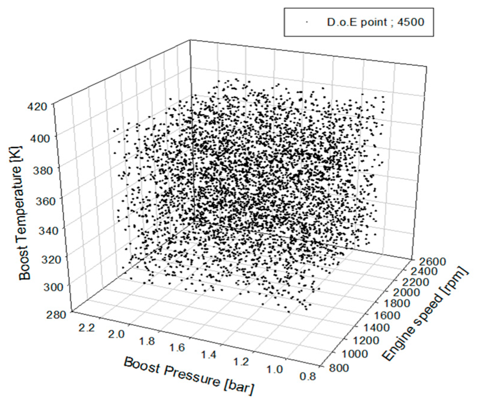
2.2. Design of Experiments (DoE)

The focus of this study is to develop a hypothetical diesel mean value engine model with sufficient accuracy and high execution speed to evaluate the control logic algorithm of the EGR system under a wide range of operating conditions. To construct the diesel mean value engine model through artificial neural network training, the design of the experiments was performed by covering a wide range of variables. In the turbocharger engine with high-pressure EGR used in this study, the main factors affecting the volumetric efficiency are the engine speed, fuel amount, fuel injection timing, EGR rate, the temperature and pressure of the turbocharger, exhaust temperature, and pressure. The range of each variable overrides the range of the variable required to satisfy the operating conditions in the mean value model. Input variables and their ranges are listed in

Table 3. Design of Experiments (DoE) input variables and ranges.

Engine Speed (rpm)	(1000–2500)
Total Fueling (mg)	(3–38)
Injection Timing (ATDC, after top dead center, deg.)	(−35–0)
Exhaust Gas Recirculation (EGR) Rate (fraction)	(0–0.39)
Boost Pressure (bar)	(1–2.5)
Boost Temperature (K)	(300–410)
Back Pressure (bar)	(1–1.35)
Back Temperature (K)	(430–770)

.

Latin hypercube sampling, an experimental design method, has the advantage of randomly assigning the sampling points by dividing the defined input range evenly. This method is very important to exclude non-practical conditions from the simulation and to obtain sufficient simulation values for learning the neural network. In this study, the physical constraints are included in the simulation design and the root mean square (RMS) error is used. As shown in Figure 3, the number of samples used in the experimental design method was selected with reference to the RMS error, and the detailed model constructed in the previous example was simulated. To reduce the number of simulations performed, the turbocharger part was removed from the detailed model. Instead, the compressor output pressure and turbine inlet pressure are input into the DoE in an over-range. This approach is useful to produce data for ANN, which is discussed in next section.

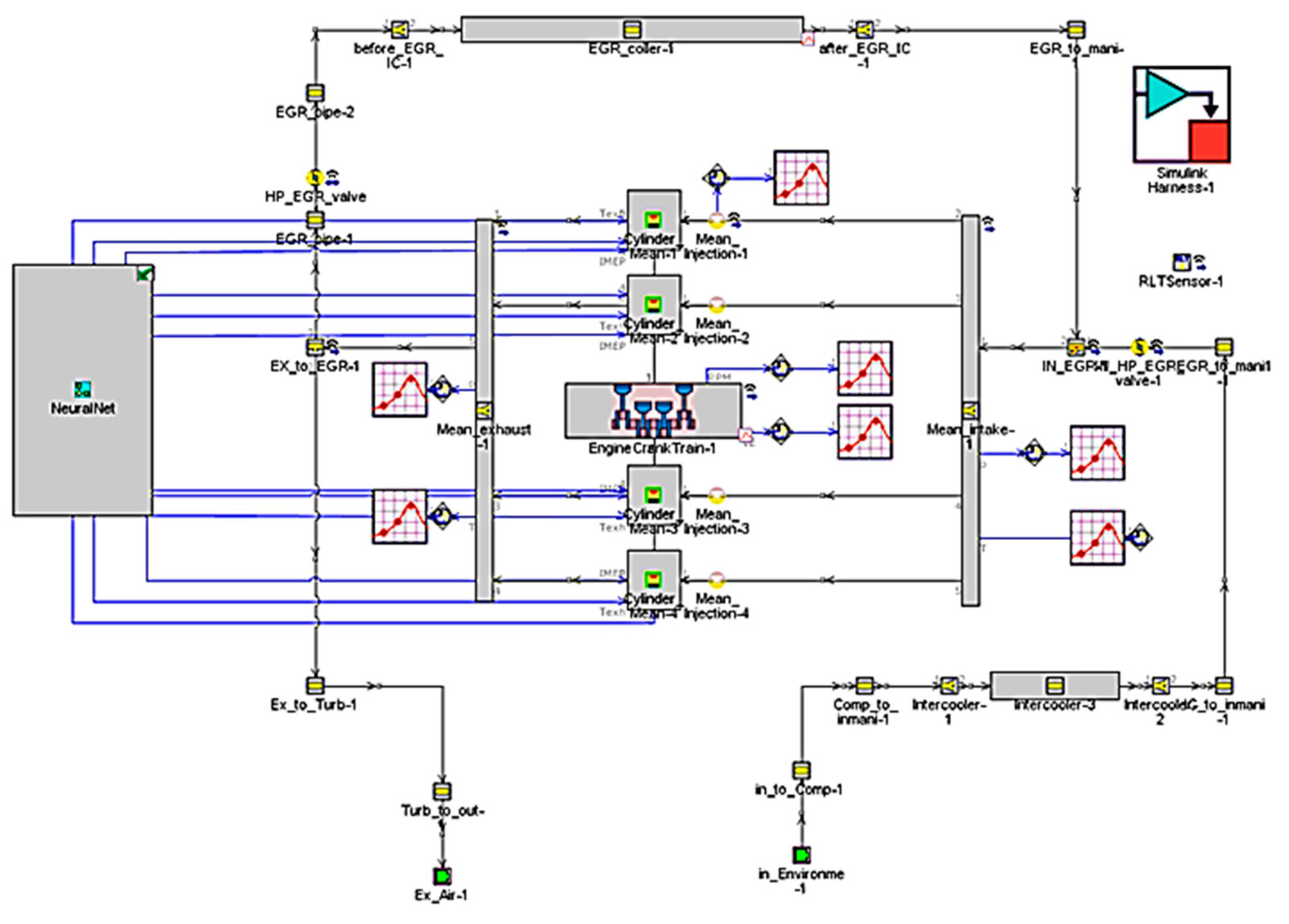
2.3. Mean Value Engine Model

The most important step in constructing the mean value model is to replace the detailed combustion model of the cylinder with a mean value cylinder model [5]. Instead of a detailed combustion model, cylinder variables such as cylinder airflow and exhaust temperature are predicted through interpolation. Alternatively, the artificial neural network method was used to predict the main performance in the cylinder efficiently and it was simplified by bundling together the flow components of the intake and exhaust manifolds. In this study, the neural network method was used to predict the main performance in the cylinder efficiently. Artificial neural network training allows intuitive recognition of the results of all input values passing through each neuron, thereby shortening the numerical analysis time. Multi-layer feed-forward is the most representative artificial neural network training method. As shown in Figure 4, the multi-layer arithmetic method is a simple method in which input values travel in only one direction, passing through neurons in each layer and obtaining the result, without circulation or feedback in the network.

The governing equations for the multilayer structure are shown in Equation (11) and the weights and characteristic values for each layer are shown in Equations (11)–(13).

Multi-layer feed forward:

$$\mathrm{y}=\mathrm{f}\left(\mathrm{w}·\mathrm{q}·\left(\mathrm{z}·\mathrm{h}\left(\mathrm{v}·\mathrm{u}+\mathrm{a}\right)+\mathrm{b}\right)+\mathrm{c}\right)$$

(11)

where, v and a are the weight and biases of the 1st layer, respectively, z and b are weight and biases of the 2nd layer, respectively, and w and c are weight and biases of the output layer, respectively. And governing equations for h and q are as follows as forms of hyperbolic tangent:

1st layer:

$$\mathrm{h}\left(\mathrm{x}\right)=-1+\frac{2}{\left(1+e^{-2\mathrm{x}}\right)}$$

(12)

2nd layer:

$$\mathrm{q}\left(\mathrm{x}\right)=-1+\frac{2}{\left(1+e^{-2\mathrm{x}}\right)}$$

(13)

In this study, the simulation result of the detailed model was used as the input value of neural network training. Several parameters (engine speed, intake manifold pressure and fuel gas fraction, exhaust manifold pressure, fuel mass, EGR rate, injection timing) were used as input values to predict the cylinder volumetric efficiency and exhaust gas temperature. The results of the artificial neural network training were included in the mean value cylinder modeling of the mean value engine model as the lower model. The average cylinder model reduced the execution speed of the overall engine model, and the complexity of the model was also reduced through the reduction of the engine model. The final mean value model includes only the main engine system components, such as four mean-valued cylinders, and a turbocharger is entered as a look-up table and includes a single flow manifold and a manifold for high-pressure EGR.

2.4. Single-Input Single-Output (SISO) Control Logic Coupled Mean Value Model

An aim of this study is to improve the responsiveness and accuracy of the reduced mean value model by combining EGR control logic. MATLAB/Simulink^®, the program used in this study for verification, has FMI standard functions and can simulate the 1D mean value model as a plant model. The EGR system of the plant model consists of a SISO algorithm with simple variable control logic. The proportional integral derivative (PID) controller, which is a general type of control strategy, was used for EGR control logic. The PID controller includes feedback; it measures the output value of the object to be controlled and compares the measured value with the reference value or desired set-point to calculate an error. Furthermore, it can calculate the control value necessary for control by using this error value. Figure 5 shows the final 1D plant model combined with Simulink.

3. Results and Discussions

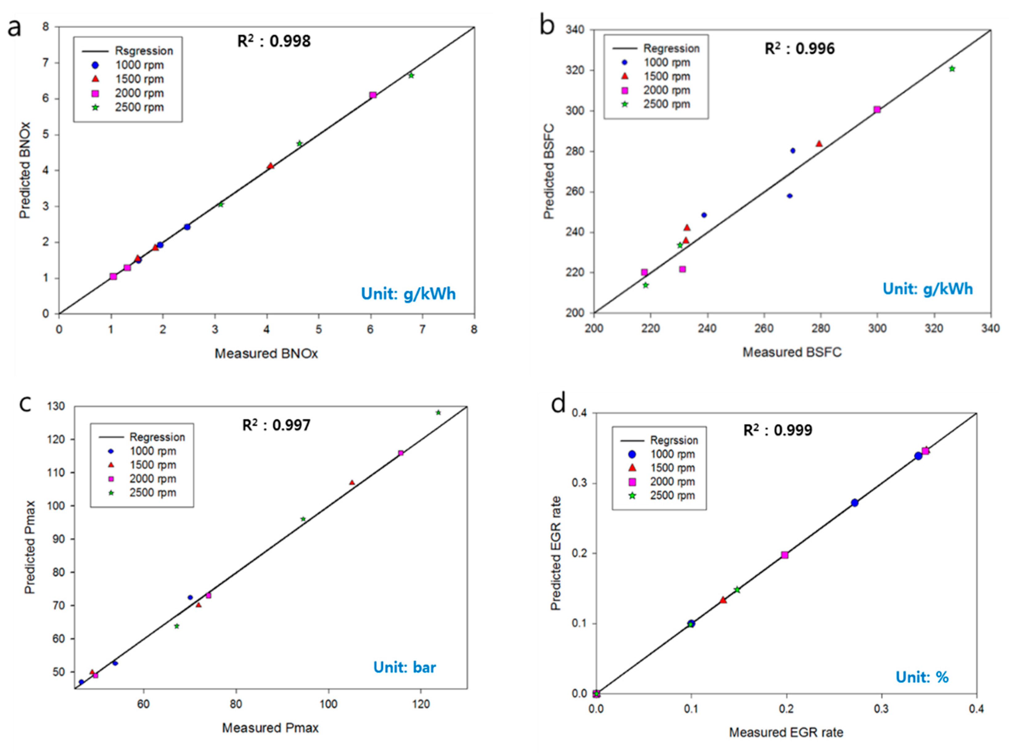
3.1. Detailed Model Validation Results and Model Reduction

To validate the model accuracy of the plant model as a final objective, the detailed model must achieve modeling accuracy under different engine speeds and load conditions. Based on the original equipment manufacturer’s test data and detailed specification of engine components implemented into the detailed engine model, the model was calibrated through DoE. The detailed model, including the engine system and the control system, has extensively verified the steady-state test results from the NEDC (New European driving cycle). Figure 6 shows the comparison between steady-state test results and simulation results in terms of BSFC (Brake specific fuel consumption), peak pressure of cylinder, EGR rate, and BNO_x (Brake specific nitric oxides), which are the main performance parameters of the engine system. The results show that the detailed model is consistent with the predicted results, showing a discrepancy within 5% on average.

The pressure and heat release rates of the engine cylinder for the operating range of the numerical analysis are also shown in Figure 7. Particularly, the heat release rate is divided into two stages, low phase and high phase, so that the heat release tendency can be observed. This is characteristic of a multi-stage compression ignition engine gradually burning through multi-stage injection. The pressure of the cylinder under the influence of this heat release rate also tends to increase at the same time as the heat rate at all operation periods. R7 > Especially for BMEP of 2 bar at every speed conditions, combustion phases are delayed due to relatively higher EGR rate having longer ignition delay for reduction of NOx under low load conditions.

The volumetric efficiency and the exhaust gas temperature, which are the main input variables of the mean value cylinder model, were predicted through artificial neural network training to construct the mean value model. The performance of the overall engine and control system was compared with that of the detailed model to determine the accuracy of the mean value engine model constructed through the artificial neural network training. R1 > Figure 8 show trained results from the artificial neural network for volumetric efficiency and exhaust gas temperature, which are used for the mean value modeling, respectively. During the neural network training process, non-meaningful data could be included due to not considered physics as the characteristics of neural network. Therefore, it is needed to constraint trained data into the meaningful data region. By comparing input data for NNT and trained results from NNT, meaningful data points could be come up with having zero error between input data and trained results as shown in the Figure 8.

Table 4. Mean value model operating condition.

Case Number	Engine Speed (rpm)	BMEP (Brake Mean Effective Pressure) (bar)	Fuel Mass Rate (cycle/mg)	Total Exhaust Gas Recirculation (EGR) Rate (%)
Case 1	1500	2	5.52	34.7
Case 2	1500	9	20.51	13.3
Case 3	1500	16	37.55	0
Case 4	2500	2	6.19	14.8
Case 5	2500	9	20.01	9.9
Case 6	2500	16	34.01	0

shows the operating conditions of the mean value model. In addition, a comparison of the numerical results of the mean value model and the detailed model is shown in Figure 9. In case 3 and case 4, the mean value model shows a lower value than the detailed model, as shown in the comparison of volumetric efficiency in Figure 9a. Furthermore, it can be observed that the air–fuel ratio at low-load and high-load operation points such as cases 1 and 4 and cases 3 and 6 has a smaller mean value than that in the detailed model. For the comparison of volumetric efficiency in Figure 9b, the mean value model at the overall operating point predicts a lower BSFC than the detailed model. In particular, case 4 shows the largest BSFC difference. This is due to the discontinuity of the trained results through random sampling. Consequently, the loss of model accuracy from the artificial neural network training results in a slight error with respect to the volumetric efficiency and the air–fuel ratio at the low-load and high-load operation points. Another reason for model accuracy loss is the injection scheme description of the mean value model. The detailed model uses multi-stage injection strategies describing the common rail direct injection system, whereas the mean value model uses a single injection description simplifying CRDI, affecting the fuel consumption rate. It is concluded that the simplification of injection strategies is an important factor in the mean value model.

3.2. Step-Transient Results with Single-Input Single-Output (SISO) Coupled Mean Value Model-in-the-Loop

Step-transient analysis was performed to confirm the applicability of SISO logic coupled by the 1D mean value model and Simulink under the model-in-the-loop environment. Describing acceleration and deceleration conditions, the RPM and EGR step-transient analyses were performed. The changes in the operating conditions and step-transient cases are summarized in

Table 5. Optimized parameter values at each conditions.

Engine Speed (rpm)	BMEP (Brake Mean Effective Pressure) (bar)	Fuel Mass Rate (cycle/mg)	Total Exhaust Gas Recirculation (EGR) Rate (%)
1500	2	5.52	34.7
2000	2	5.81	34.6
2000	9	19.33	19.8
2500	9	20.01	9.9
2500	16	34.01	0

and shown in Figure 10 and Figure 11.

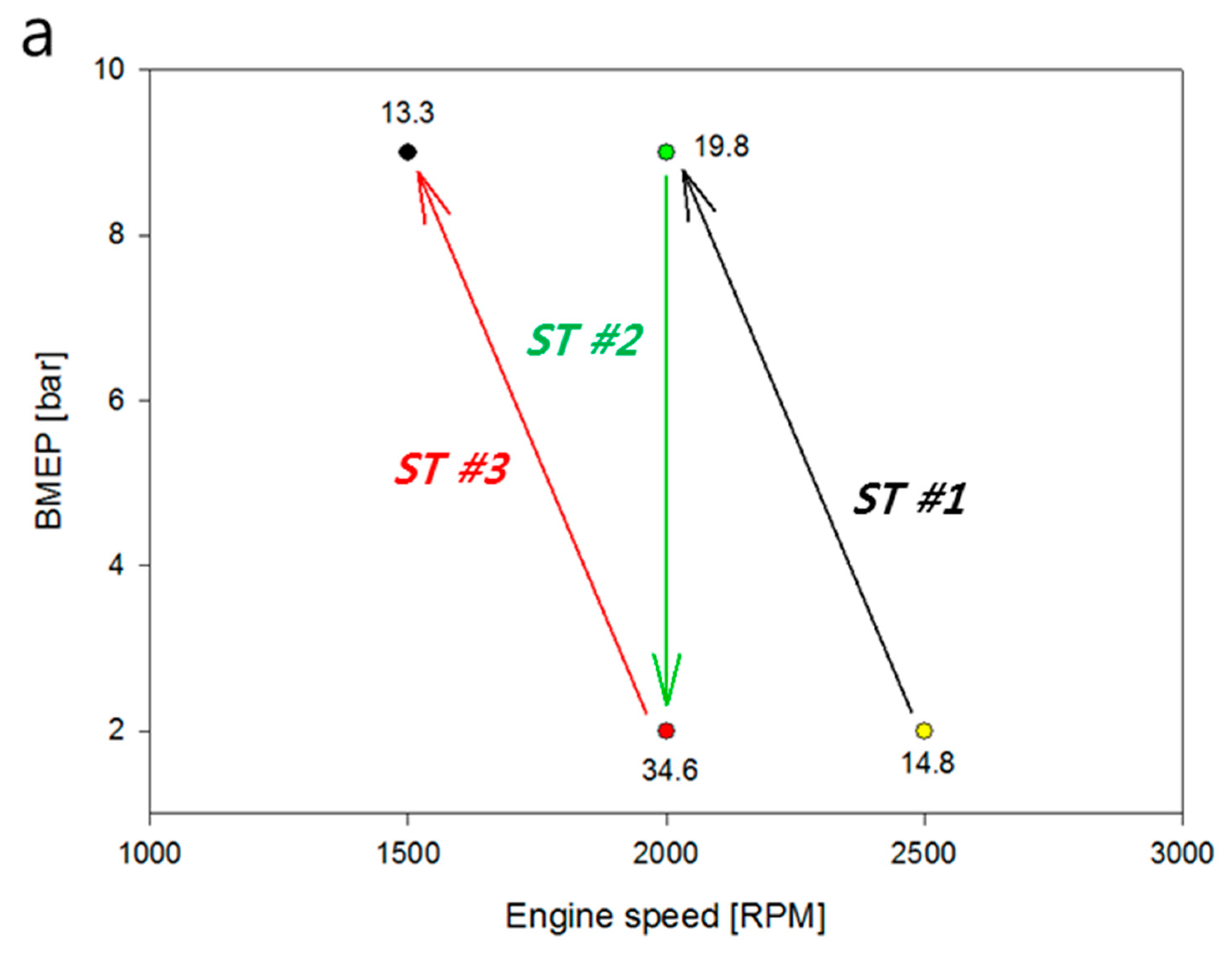
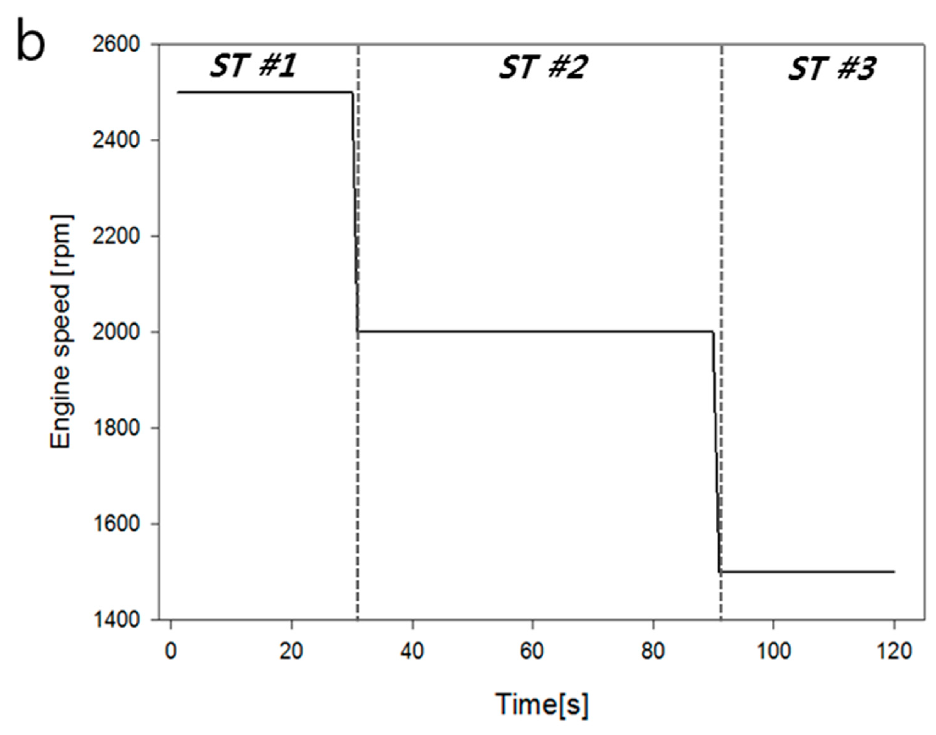
3.2.1. Step-Transient for Acceleration

Figure 12 shows the volumetric efficiency and EGR rate change over time under acceleration conditions. In ST # 1, the overshot can be confirmed from 0 to 8 s. This is the response characteristic of the controller because the proportional band of the PID controller is narrow. In addition, as shown in Figure 12a, which is a comparative graph of volumetric efficiency, the volumetric efficiency of ST # 1 is achieved smoothly without large hunting between 0 and 3 s, and the target EGR rate from Figure 12b is achieved at a similar target EGR rate of 3.6 s. In ST # 2, the EGR rate is similar but the speed is accelerated, and hence, undershoot can be checked for 10 s. In the volumetric efficiency of Figure 12a, the SISO coupled mean value model shows undershoot after a slight increase in 10 s. Another reason is the response characteristic owing to the large integration time of the PID controller. However, after 30 s, the control response is stabilized, and the target EGR rate is achieved. Therefore, there is a delay in the response speed of the control system attributed to the error in the gain coefficients of the PID controller even in the ST # 3 and ST # 4 sections. However, the EGR rate reaches a desired target value within 10 s in all the step phases. The volumetric efficiency was also varied in the step boundary affected by the EGR rate changes. However, its response is stabilized in a short time compared with the EGR rate.

3.2.2. Step-Transient for Deceleration

Figure 13 shows the volumetric efficiency and EGR rate change over time under deceleration conditions. Unlike the acceleration condition, the deceleration condition can confirm undershooting at all speeds and EGR rates. Especially, ST # 1 achieved the target EGR rate in 8 s, but in the case of ST # 2, the EGR rate dropped to 10 for approximately 3 s after 30 s. For ST # 2, the EGR rate dropped to 10 for 30 s to approximately 3 s owing to volumetric efficiency, but with volumetric efficiency, the EGR rate was achieved after 33 s. In ST # 3, where the EGR rate is sharply reduced, the target EGR rate is achieved relatively fast compared with that in the other sections, although there is a response delay. Consequently, the rapid EGR rate change affected the response speed, which slowed the response time and also affected the high convergence time. However, it is shown that the target value is reached within 10 s at all speeds and EGR rate change intervals, and that the control target of the PID controller has converged to the steady-state error. Furthermore, the volumetric efficiency shows a similar shape to the mean value model.

3.3. Model Accuracy and Execution Speed Trade-off

The trade-off between the model accuracy and execution speed was compared for the detailed model, mean value model, and SISO coupled mean value model. Figure 14 compares the model prediction accuracy and numerical analysis execution speed. The mean value model constructed using an artificial neural network shows an accuracy loss of approximately 3% compared with the detailed model. This is mainly due to the lack of sampling points for the training of volumetric efficiency and exhaust gas temperature. However, the execution speed of the mean value model and the SISO coupled mean value model is approximately two times greater than that of the detailed model. Consequently, the SISO coupled mean value model has slightly lower model accuracy but higher analysis speed than the detailed model and the mean value model without SISO coupling. It is concluded that the SISO coupled mean value model has a good balance between model accuracy and execution speed.

4. Conclusions

In this study, the model reduction process was performed through artificial neural network training by constructing a virtual plant model for real-time numerical analysis, and the response characteristic of EGR logic was investigated through step-transient simulation by combining the mean value model and EGR logic. The conclusions drawn are as follows.

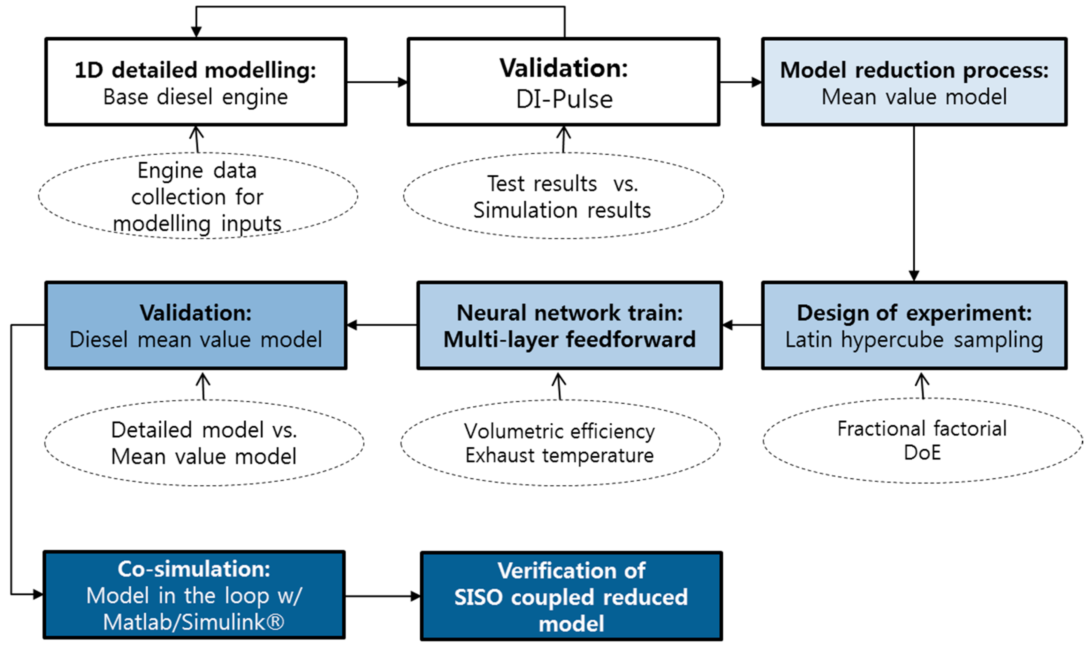
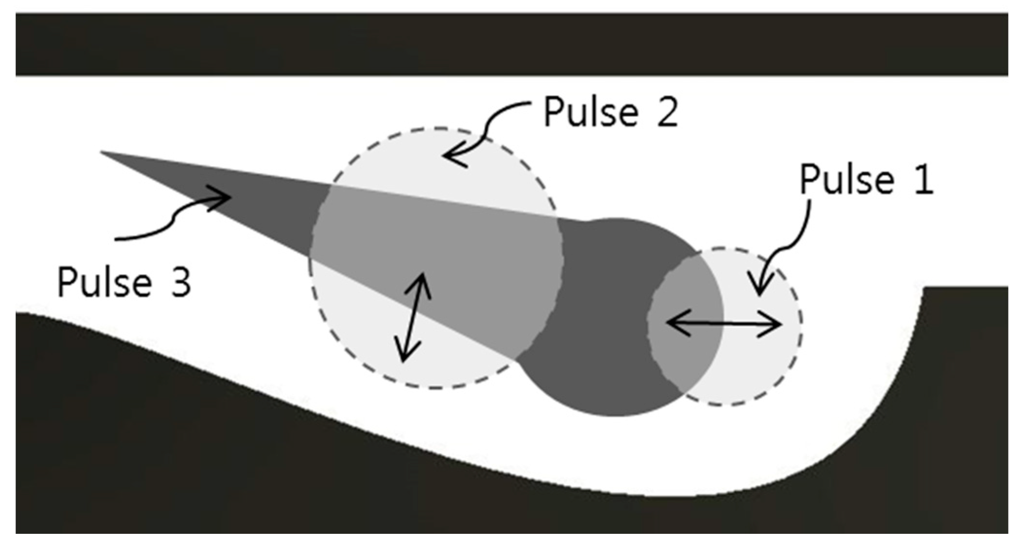
• A detailed model was constructed using the DI-pulse mode to describe the diesel combustion mode to construct the base model of the plant model. The four correction multipliers of the DI-pulse mode were optimized for each operating point using the Latin hypercube method.
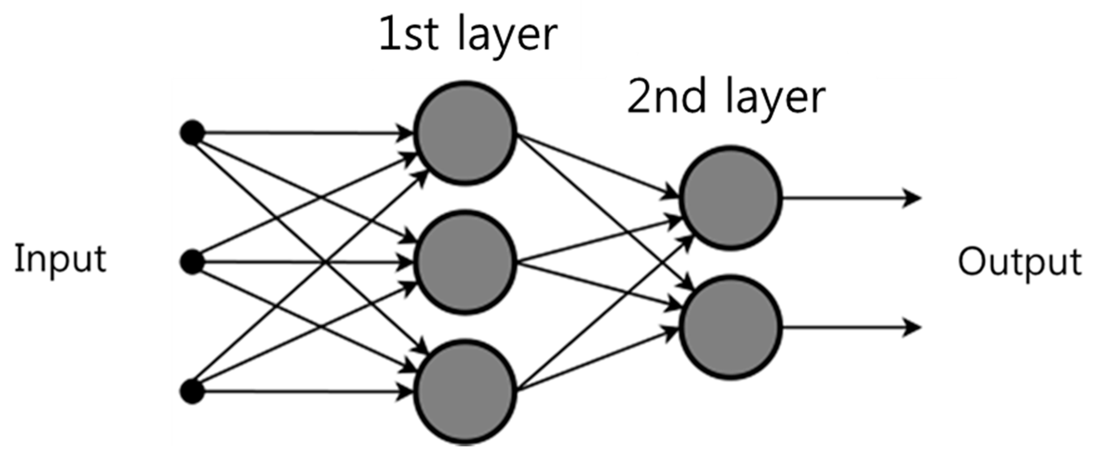
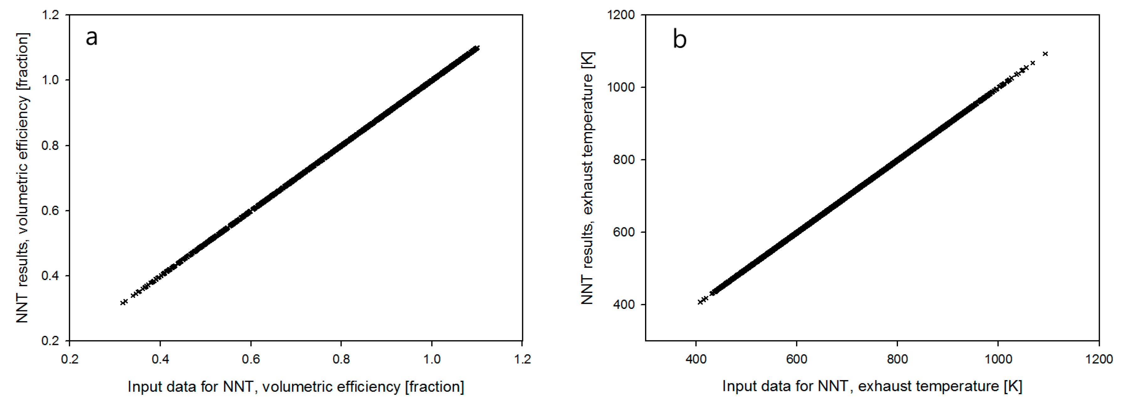
• The diesel mean-valued engine model was simplified by bundling together the flow components of the intake and exhaust manifolds. Artificial neural networks were also used to approximate the simulation results of the detailed model for the input variables—i.e., the volumetric efficiency and the exhaust gas temperature—of the mean value cylinder model. The artificial neural network training method uses a multi-layer feed-forward method that calculates results simply without circulation. As shown in Figure 8 for the exhaust gas temperature, the simulated values of the detailed model were not sufficient and the 1200–1400 K range of the exhaust gas temperature training could not be predicted.
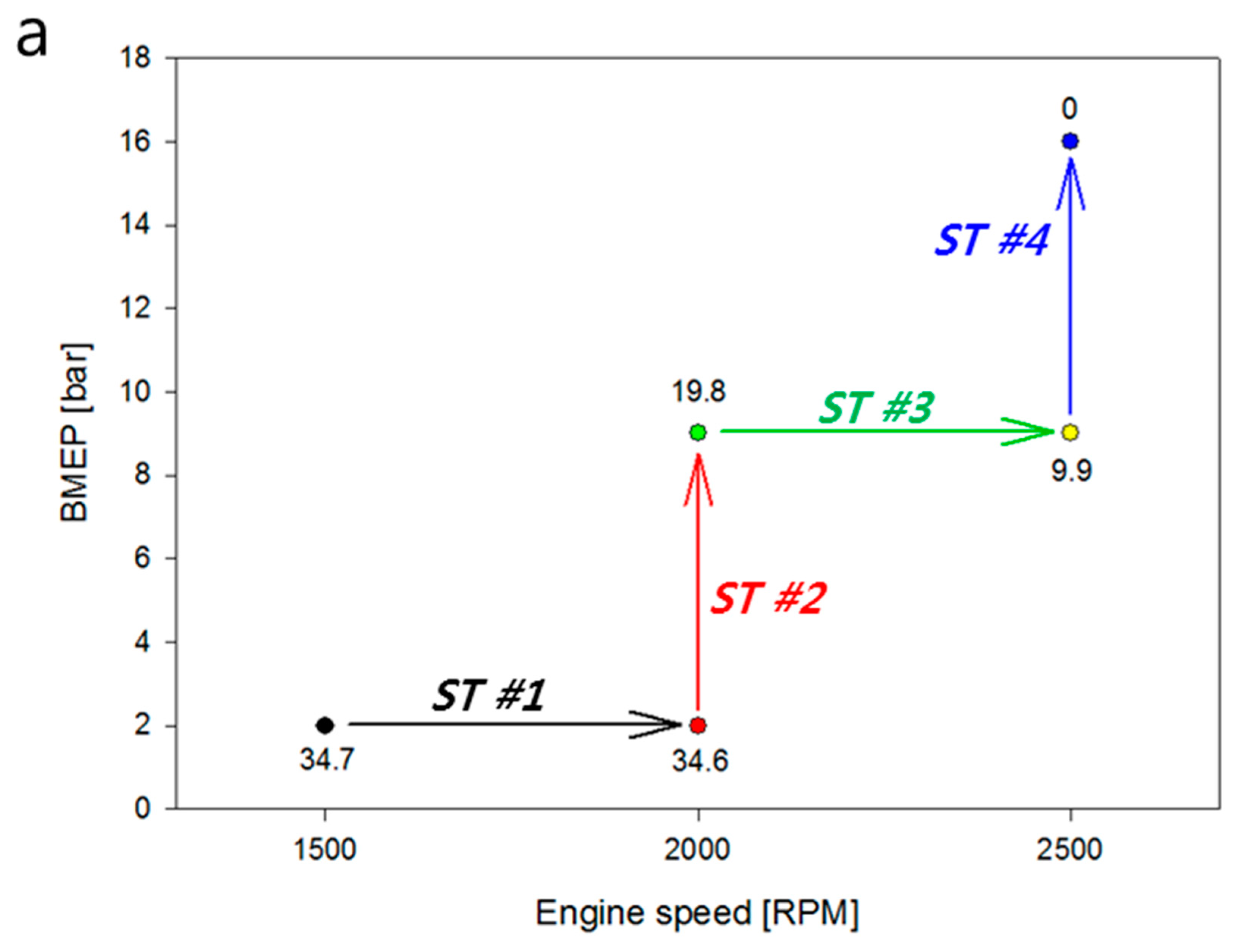
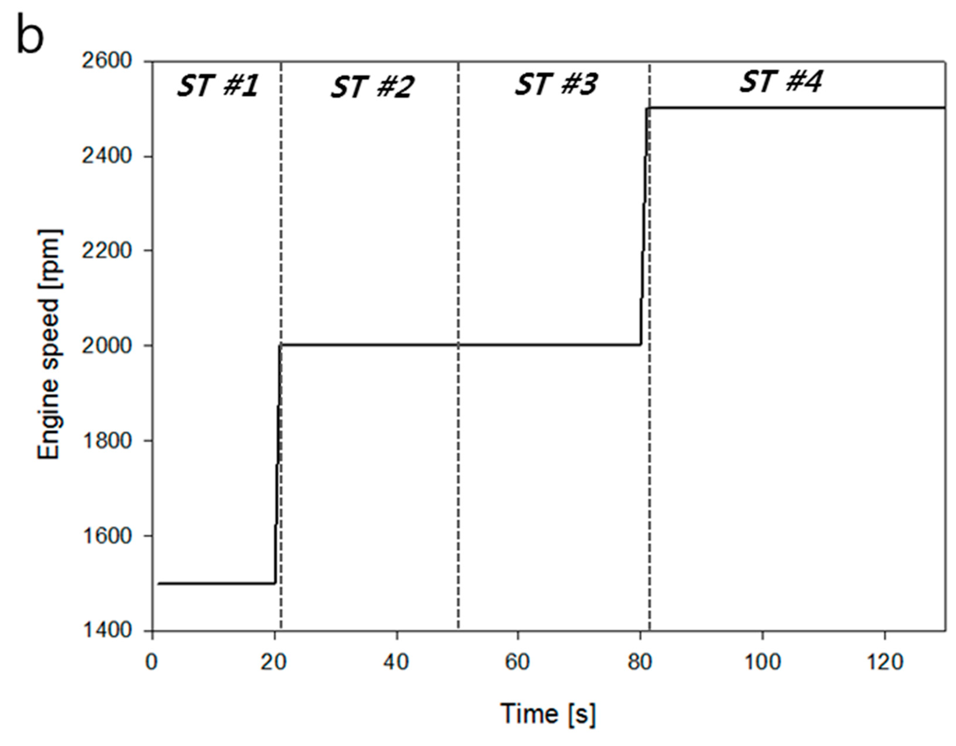
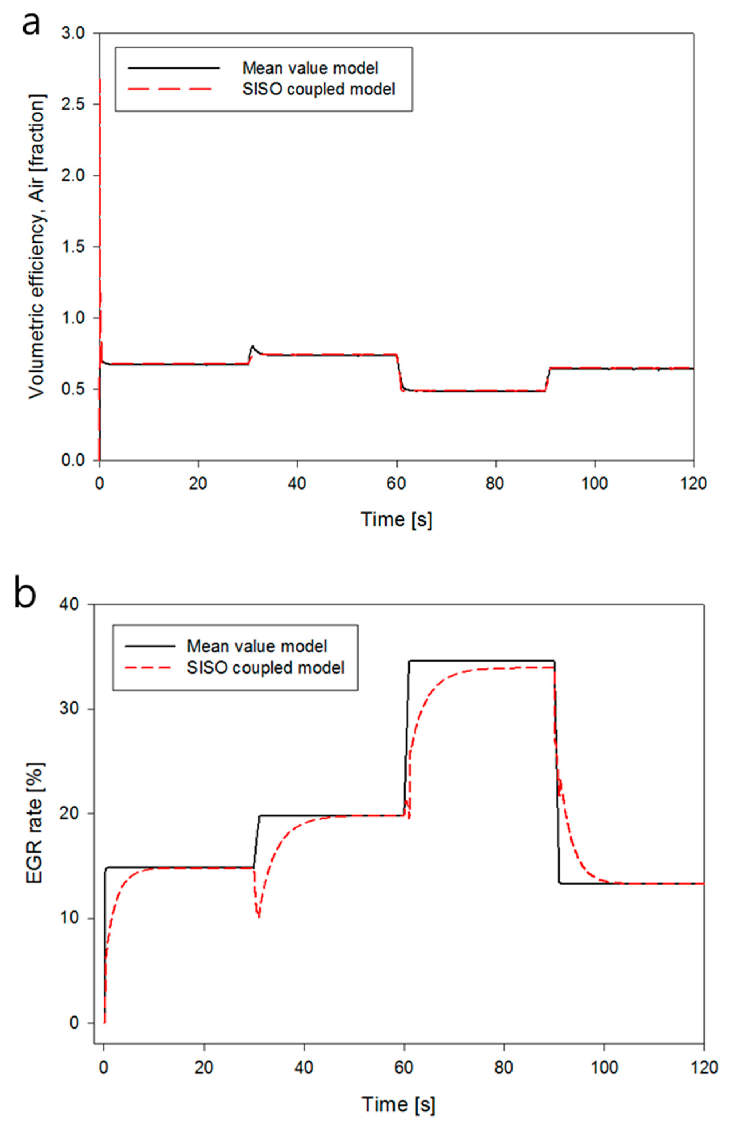
• Acceleration condition description simulation allows model-based control to follow the target value well. However, as shown in Figure 12, the EGR ratio showed overshoot and undershoot owing to slight changes in the volumetric efficiency over the initial 10 s in the ST # 1 and ST # 2 zones. This response characteristic appears because the proportional band of the PID controller is narrow and the integration time is long. All the sections have a response delay but the target EGR percentage value is reached within 10 s.
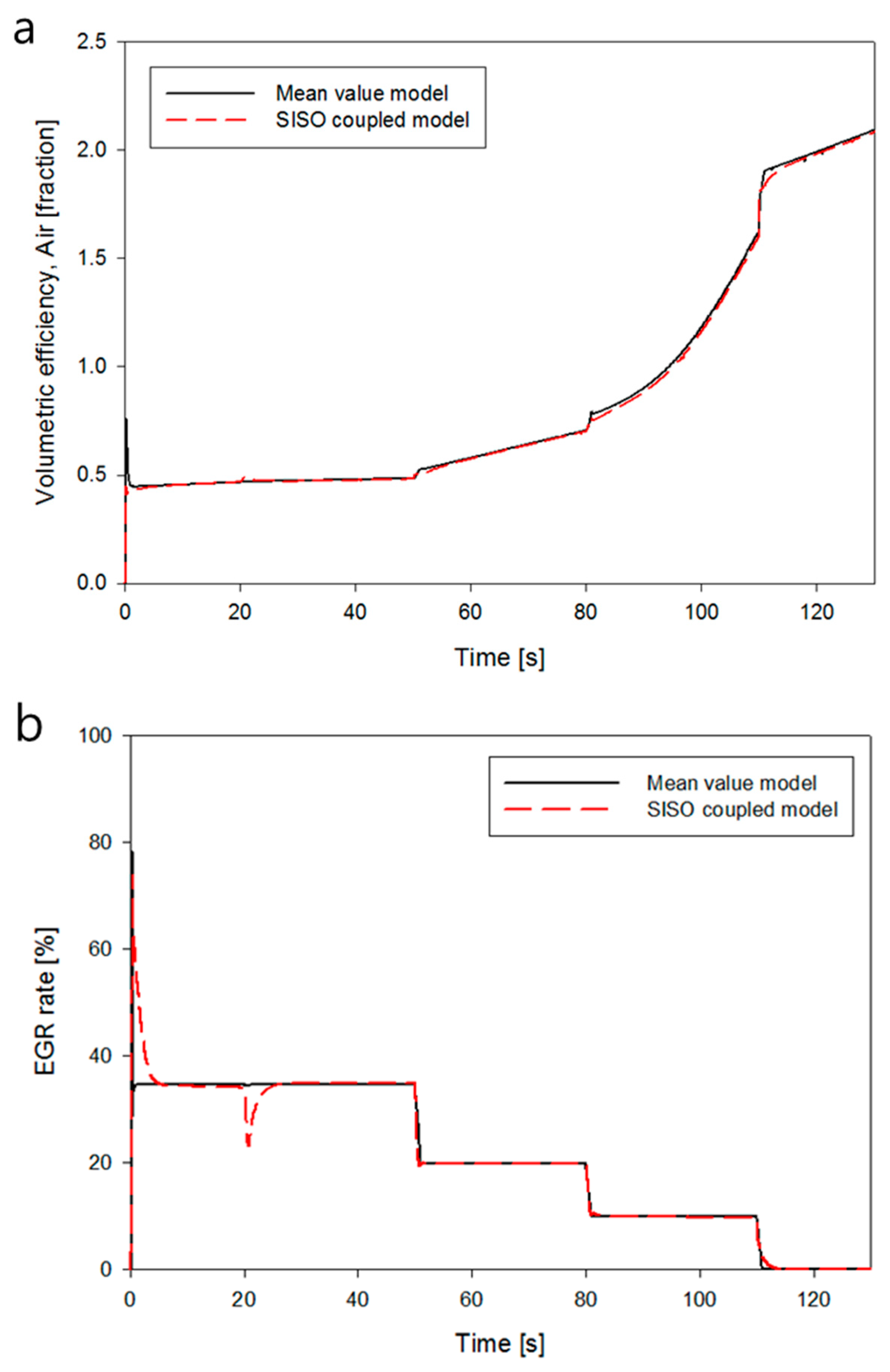
• The response characteristics of the EGR logic were confirmed through the simulation of the deceleration condition with complex changes. As shown in Figure 13a, unlike in the case of the acceleration conditions, the volumetric efficiency can confirm the undershoot response characteristics in the entire speed change period. Moreover, the tendency of undershoot is larger than the change in the acceleration condition. This indicates that the PID controller responds slowly but weakly owing to its weak motion.
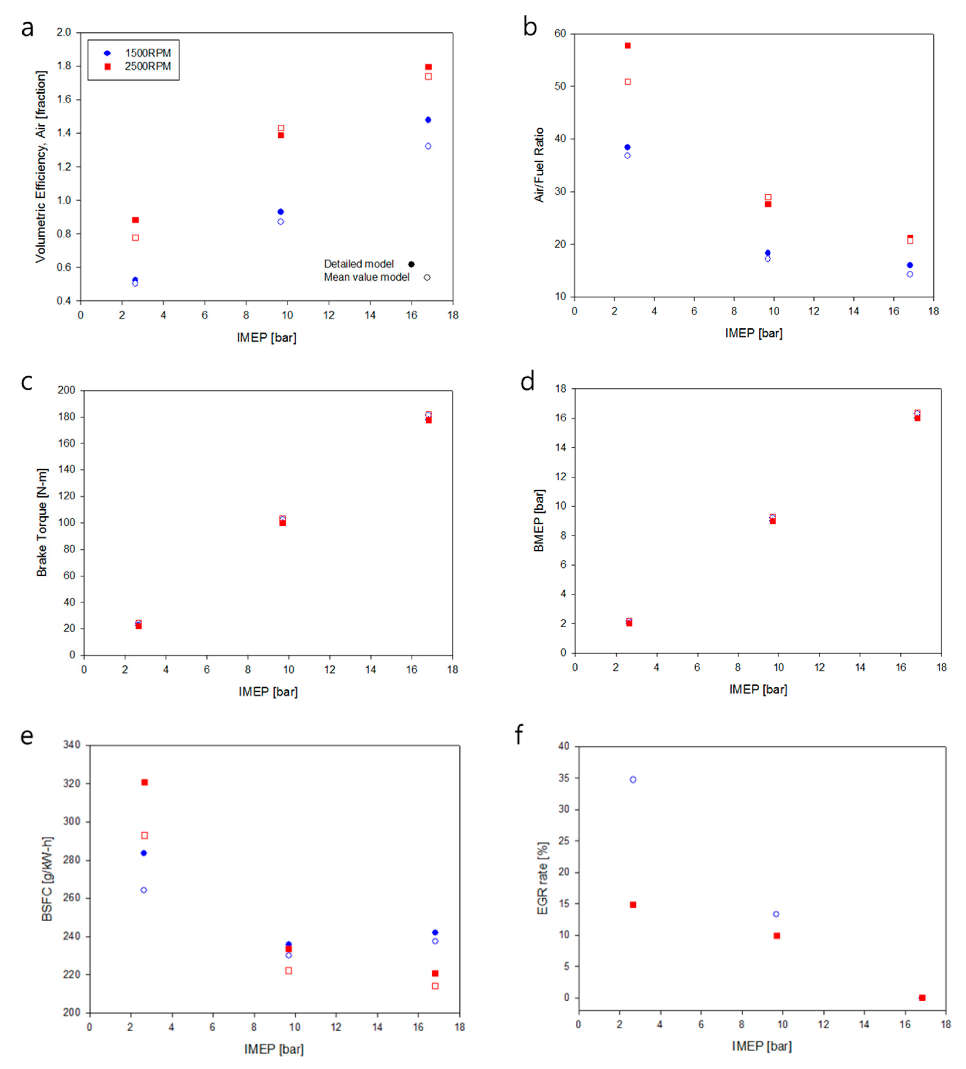
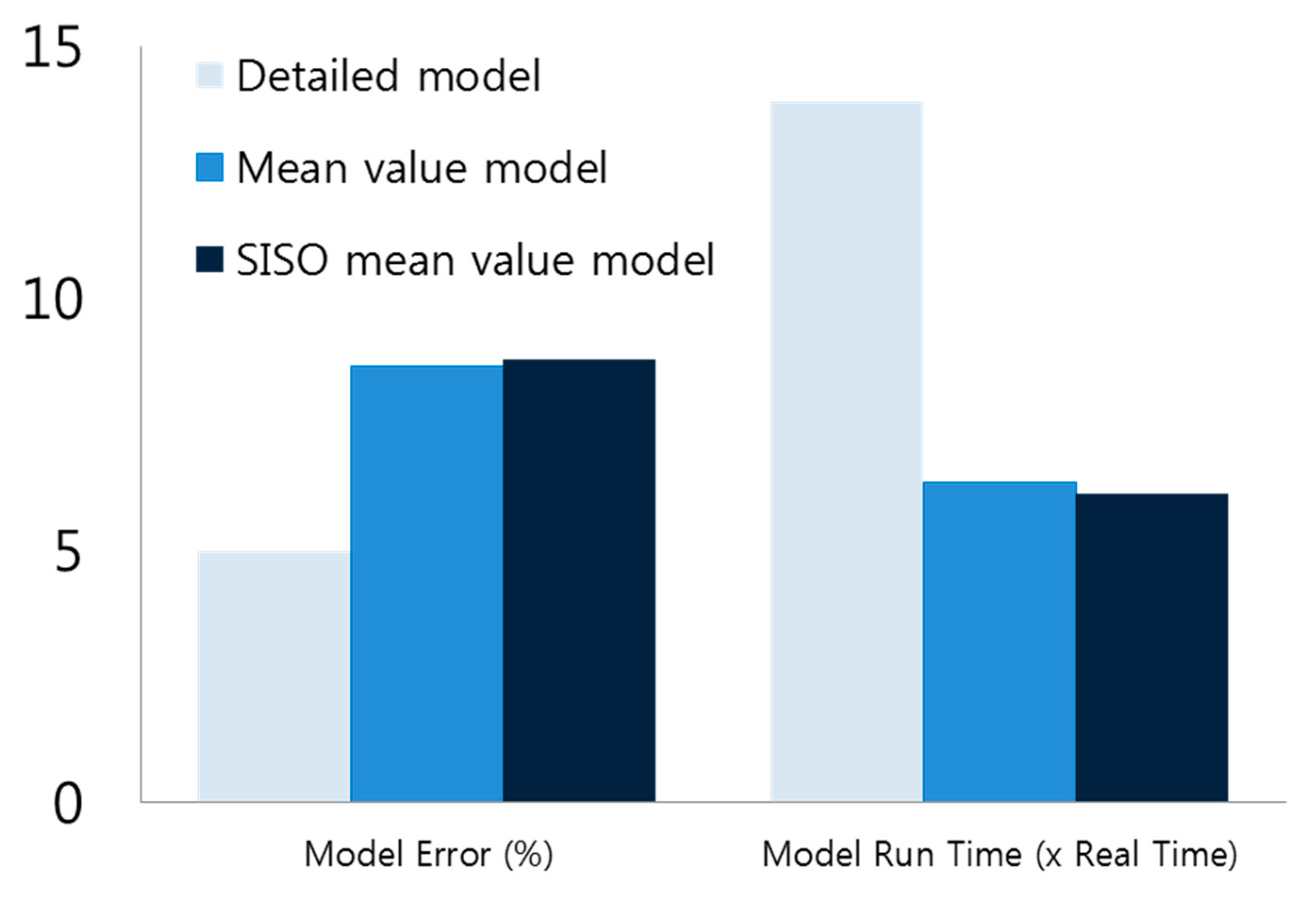
• The accuracy of the diesel average value model in Figure 14 showed a loss of approximately 3%, owing to the volumetric efficiency loss of the cylinder when compared with that of the diesel detailed model. However, in the case of the simulation run-time of the mean value model, the flow component shortening of the intake/manifold and the artificial neural network reduce the engine performance by approximately two times because of the intuitive prediction of the engine’s main performance parameters. Furthermore, the SISO coupled mean value model constructed in the study has a good balance between model accuracy and execution speed.

References

1. Heidrich, L.; Shyrokau, B.; Savitski, D.; Ivanov, V.; Augsburg, K.; Wang, D. Hardware-in-the-loop test rig for integrated vehicle control systems. IFAC Proc. Vol. 2013, 46, 683–688. [Google Scholar] [CrossRef]
2. Yu, M.X.; Tang, X.Y.; Lin, Y.Z.; Wang, X.Z. Diesel engine modeling based on recurrent neural networks for a hardware-in-the-loop simulation system of diesel generator sets. Neurocomputing 2018, 283, 9–19. [Google Scholar] [CrossRef]
3. Yi, L.; He, H.; Peng, J. Hardware-in-loop simulation for the energy management system development of a plug-in hybrid electric bus. Energy Procedia 2016, 88, 950–956. [Google Scholar] [CrossRef]
4. Maroteaux, F.; Saad, C. Combined mean value engine model and crank angle resolved in-cylinder modeling with NOx emissions model for real-time Diesel engine simulations at high engine speed. Energy 2015, 88, 515–527. [Google Scholar] [CrossRef]
5. He, Y.; Lin, C.-C. Development and Validation of a Mean Value Engine Model for Integrated Engine and Control System Simulation; SAE Technical Paper; SAE: Troy, MI, USA, 2007. [Google Scholar]
6. Lujan, J.M.; Climent, H.; Garcia-Cuevas, L.M.; Moratal, A. Volumetric efficiency modelling of internal combustion engines based on a novel adaptive learning algorithm of artificial neural networks. Appl. Therm. Eng. 2017, 123, 625–634. [Google Scholar] [CrossRef]
7. Uzun, A. Air mass flow estimation of diesel engines using neural network. Fuel 2014, 117, 833–838. [Google Scholar] [CrossRef]
8. Zarghami, M.; Hosseinnia, S.H.; Babazadeh, M. Optimal Control of EGR System in Gasoline Engine Based on Gaussian Process. IFAC-Pap. Online 2017, 50, 3750–3755. [Google Scholar] [CrossRef]
9. Roy, S.; Banerjee, R.; Bose, P.K. Performance and exhaust emissions prediction of a CRDI assisted single cylinder diesel engine coupled with EGR using artificial neural network. Appl. Energy 2014, 119, 330–340. [Google Scholar] [CrossRef]
10. Theotokatos, G.; Guan, C.; Chen, H.; Lazakis, I. Development of an extended mean value engine model for predicting the marine two-stroke engine operation at varying settings. Energy 2018, 143, 533–545. [Google Scholar] [CrossRef] [Green Version]
11. Turkson, R.F.; Yan, F.; Ali, M.K.A.; Hu, J. Artificial neural network applications in the calibration of spark-ignition engines: An overview, Engineering Science and Technology. Int. J. 2016, 19, 1346–1359. [Google Scholar]
12. Isermann, R.; Sequenz, H. Model-based development of combustion-engine control and optimal calibration for driving cycles: General procedure and application. IFAC-Pap. Online 2016, 49, 633–640. [Google Scholar] [CrossRef]
13. Li, W.L.; Zhang, X.B.; Li, H.M. Co-simulation platforms for co-design of networked control systems: An overview. Control Eng. Pract. 2014, 23, 44–56. [Google Scholar] [CrossRef]
14. Quaglia, D.; Muradore, R.; Bragantini, R.; Fiorini, P. A SystemC/Matlab co-simulation tool for networked control systems. Simul. Model. Pract. Theory 2012, 23, 71–86. [Google Scholar] [CrossRef]
15. Rao, K.D. Modeling, simulation and control of semi active suspension system for automobiles under matlab simulink using pid controller. IFAC Proc. Vol. 2014, 47, 827–831. [Google Scholar] [CrossRef]
16. Casoli, P.; Gambarotta, A.; Pompini, N.; Riccò, L. Development and application of co-simulation and “control-oriented” modeling in the improvement of performance and energy saving of mobile machinery. Energy Procedia 2014, 45, 849–858. [Google Scholar] [CrossRef]
17. Xie, H.; Li, S.; Song, K.; He, G. Model-based decoupling control of VGT and EGR with active disturbance rejection in diesel engines. IFAC Proc. Vol. 2013, 46, 282–288. [Google Scholar] [CrossRef]
18. Cieslar, D.; Dickinson, P.; Darlington, A.; Glover, K.; Collings, N. Model based approach to closed loop control of 1-D engine simulation models. Control Eng. Pract. 2014, 29, 212–224. [Google Scholar] [CrossRef]
19. Nylén, A.; Henningsson, M.; Cervin, A.; Tunestál, P. Control Design Based on FMI: A Diesel Engine Control Case Study. IFAC-Pap. Online 2016, 49, 231–238. [Google Scholar]
20. Gupta, H.N. Fundamentals of Internal Combustion Engines; PHI Learning Pvt. Ltd.: Delhi, India, 2012. [Google Scholar]
21. Miller, R.; Davis, G.; Lavoie, G.; Newman, C.; Gardner, T. A Super-Extended Zel’dovich Mechanism for NOx Modeling and Engine Calibration; SAE Transactions: Troy, MI, USA, 1998; pp. 1090–1100. [Google Scholar]
22. Park, S.; Song, S. Model-based multi-objective Pareto optimization of the BSFC and NOx emission of a dual-fuel engine using a variable valve strategy. J. Nat. Gas Sci. Eng. 2017, 39, 161–172. [Google Scholar] [CrossRef]
Figure 1. Overall research flow of the present study.
Energies 12 02823 g001
Figure 2. Multi-pulse model in GT (Gamma technologies)-Power.
Energies 12 02823 g002
Figure 3. Design of Experiments (DoE) point for direct-injection diesel multi-pulse (DI-Pulse) correction multiplier optimization.
Energies 12 02823 g003
Figure 4. Multi-layer feed forward.
Energies 12 02823 g004
Figure 5. Single-input single-output (SISO) coupled mean value model.
Energies 12 02823 g005
Figure 6. Comparison between measured result and predicted result for. (a) BNOx, g/kWh; (b) BSFC, g/kWh; (c) Pmax, bar; (d) exhaust gas recirculation (EGR) rate, %.
Energies 12 02823 g006
Figure 7. In-cylinder pressure and gross heat release rate of detailed model (a) 1000 rpm (b) 1500 rpm, (c) 2000 rpm, (d) 2500 rpm.
Energies 12 02823 g007aEnergies 12 02823 g007b
Figure 8. Input data for NNT (Neural network training) and trained results of (a) volumetric efficiency, (b) exhaust temperature for mean values modeling.
Energies 12 02823 g008
Figure 9. Comparison between detailed model result and mean value model result for (a) volumetric efficiency, (b) air/fuel ratio, (c) brake torque, (d) BMEP (Brake mean effective pressure), (e) BSFC, (f) EGR rate.
Energies 12 02823 g009
Figure 10. Acceleration step transient conditions wrt (a) engine speed vs. BMEP, (b) time vs. engine speed.
Energies 12 02823 g010aEnergies 12 02823 g010b
Figure 11. Deceleration step transient conditions wrt (a) engine speed vs. BMEP, (b) time vs. engine speed.
Energies 12 02823 g011aEnergies 12 02823 g011b
Figure 12. Comparison between mean value model result and single-input single-output (SISO) coupled MVM (Mean value model) at acceleration step transient conditions for (a) volumetric efficiency, (b) EGR rate.
Energies 12 02823 g012
Figure 13. Comparison between mean value model result and single-input single-output (SISO) coupled MVM (Mean value model) at deceleration step transient conditions for (a) volumetric efficiency, (b) EGR rate.
Energies 12 02823 g013
Figure 14. Trade-off of model error model run time: y-axis represent for the absolute value for both model error and run time.
Energies 12 02823 g014