Analysis of Thermodynamic Models for Simulation and Optimisation of Organic Rankine Cycles


Abstract
:1. Introduction
2. Methodology
3. Results
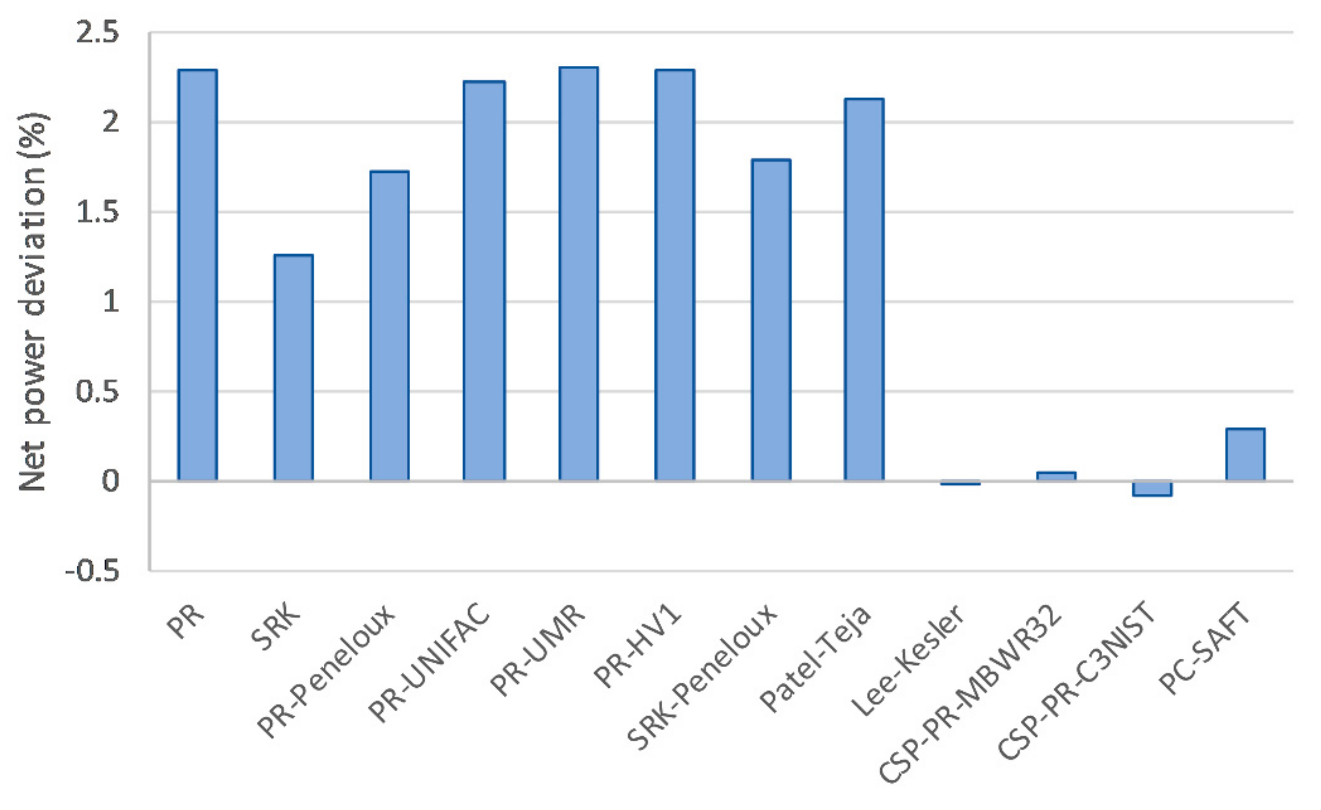
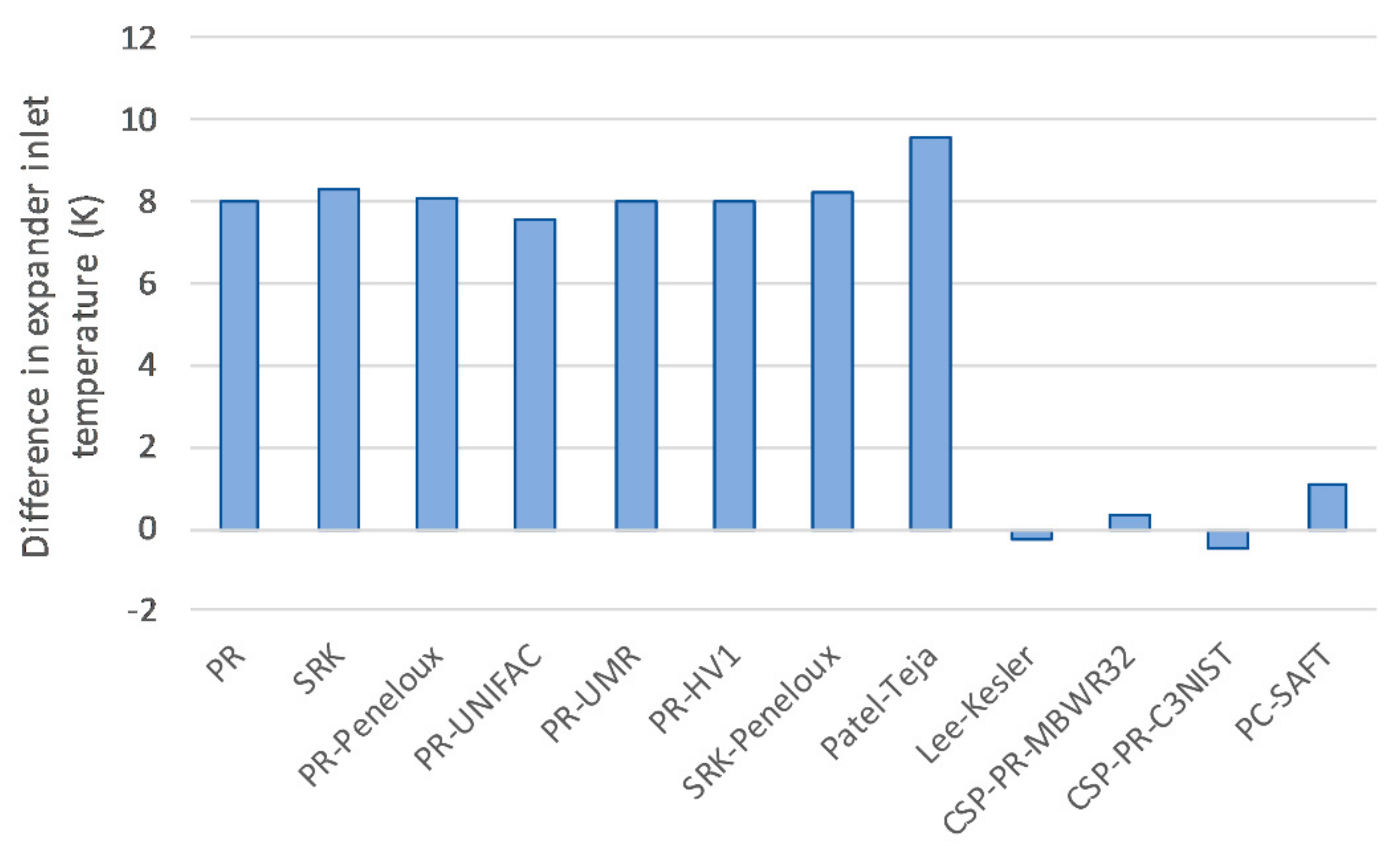
3.1. Accuracy
3.2. Computational Time
3.3. Robustness
3.4. Overall
4. Conclusions
Author Contributions
Funding
Acknowledgments
Conflicts of Interest
Nomenclature
| Specific enthalpy | kJ/kg | |
| Mass flow | kg/s | |
| Pressure | bar | |
| Temperature | °C | |
| Net power | kW |
Abbreviations
| WHRU | Waste heat recovery unit |
| Subscripts | |
| 1 | Condenser outlet |
| 2 | WHRU inlet |
| 3 | Turbine inlet |
| 4 | Turbine outlet |
| 5 | Condenser inlet |
| ref | Reference |
| wf | Working fluid |
References
- Frutiger, J.; Andreasen, J.; Liu, W.; Spliethoff, H.; Haglind, F.; Abildskov, J.; Sin, G. Working fluid selection for organic Rankine cycles—Impact of uncertainty of fluid properties. Energy 2016, 109, 987–997. [Google Scholar] [CrossRef]
- Stijepovic, M.Z.; Linke, P.; Papadopoulos, A.I.; Grujic, A.S. On the role of working fluid properties in Organic Rankine Cycle performance. Appl. Therm. Eng. 2012, 36, 406–413. [Google Scholar] [CrossRef]
- Mazzoccoli, M.; Bosio, B.; Arato, E.; Brandani, S. Comparison of equations-of-state with P-ρ-T experimental data of binary mixtures rich in CO2 under the conditions of pipeline transport. J. Supercrit. Fluids 2014, 95, 474–490. [Google Scholar] [CrossRef]
- Li, H.; Yan, J. Evaluating cubic equations of state for calculation of vapor–liquid equilibrium of CO2 and CO2-mixtures for CO2 capture and storage processes. Appl. Energy 2009, 86, 826–836. [Google Scholar] [CrossRef]
- Li, H.; Yan, J. Impacts of equations of state (EOS) and impurities on the volume calculation of CO2 mixtures in the applications of CO2 capture and storage (CCS) processes. Appl. Energy 2009, 86, 2760–2770. [Google Scholar] [CrossRef]
- Abdollahi-Demneh, F.; Moosavian, M.A.; Montazer-Rahmati, M.M.; Omidkhah, M.R.; Bahmaniar, H. Comparison of the prediction power of 23 generalized equations of state: Part I. Saturated thermodynamic properties of 102 pure substances. Fluid Phase Equilib. 2010, 288, 67–82. [Google Scholar] [CrossRef]
- Liu, K.; Wu, Y.; McHugh, M.A.; Baled, H.; Enick, R.M.; Morreale, B.D. Equation of state modeling of high-pressure, high-temperature hydrocarbon density data. J. Supercrit. Fluids 2010, 55, 701–711. [Google Scholar] [CrossRef]
- Orbey, H.; Sandler, S.I. A comparison of various cubic equation of state mixing rules for the simultaneous description of excess enthalpies and vapor-liquid equilibria. Fluid Phase Equilib. 1996, 121, 67–83. [Google Scholar] [CrossRef]
- Brown, J.S. Predicting performance of refrigerants using the Peng–Robinson Equation of State. Int. J. Refrig. 2007, 30, 1319–1328. [Google Scholar] [CrossRef]
- Kuboth, S.; Neubert, M.; Preißinger, M.; Brüggemann, D. Iterative Approach for the Design of an Organic Rankine Cycle based on Thermodynamic Process Simulations and a Small-Scale Test Rig. Energy Procedia 2017, 129, 18–25. [Google Scholar] [CrossRef]
- Wilhelmsen, Ø.; Aasen, A.; Skaugen, G.; Aursand, P.; Austegard, A.; Aursand, E.; Gjennestad, M.A.; Lund, H.; Linga, G.; Hammer, M. Thermodyn. Model. Equ. State Present Chall. Establ. Methods 2017, 56, 3503–3515.
- Schittkowski, K. NLPQL: A FORTRAN subroutine for solving constrained nonlinear programming problems. Ann. Oper. Res. 1986, 5, 485–500. [Google Scholar] [CrossRef]
- Skaugen, G.; Hammer, M.; Wahl, P.E.; Wilhelmsen, Ø. Constrained non-linear optimisation of a process for liquefaction of natural gas including a geometrical and thermo-hydraulic model of a compact heat exchanger. Comput. Chem. Eng. 2015, 73, 102–115. [Google Scholar] [CrossRef]
- Aasen, A.; Hammer, M.; Skaugen, G.; Jakobsen, J.P.; Wilhelmsen, Ø. Thermodynamic models to accurately describe the PVTxy-behavior of water/carbon dioxide mixtures. Fluid Phase Equilib. 2017, 442, 125–139. [Google Scholar] [CrossRef]
- Ibrahim, M.; Skaugen, G.; Ertesvåg, I.S.; Haug-Warberg, T. Modeling CO2-water mixture thermodynamics using various equations of state (EoSs) with emphasis on the potential of the SPUNG EoS. Chem. Eng. Sci. 2014, 113, 22–34. [Google Scholar] [CrossRef]
- Younglove, B.A.; Ely, J. Thermophysical Properties of Fluids. II. Methane, Ethane, Propane, Isobutane, and Normal Butane. J. Phys. Chem. Ref. Data 1987, 16, 577–798. [Google Scholar] [CrossRef]
- Lemmon, E.W.; McLinden, M.O.; Wagner, W. Thermodynamic Properties of Propane. III. A Reference Equation of State for Temperatures from the Melting Line to 650 K and Pressures up to 1000 MPa. J. Chem. Eng. Data 2009, 54, 3141–3180. [Google Scholar] [CrossRef]
- Peng, D.-Y.; Robinson, D.B. A New Two-Constant Equation of State. Ind. Eng. Chem. Fundam. 1976, 15, 59–64. [Google Scholar] [CrossRef]
- Kunz, O.; Wagner, W. The GERG-2008 Wide-Range Equation of State for Natural Gases and Other Mixtures: An Expansion of GERG-2004. J. Chem. Eng. Data 2012, 57, 3032–3091. [Google Scholar] [CrossRef]
- Soave, G. Equilibrium constants from a modified Redlich-Kwong equation of state. Chem. Eng. Sci. 1972, 27, 1197–1203. [Google Scholar] [CrossRef]
- Jhaveri, B.S.; Youngren, G.K. Three-Parameter Modification of the Peng-Robinson Equation of State to Improve Volumetric Predictions. SPE Reserv. Eng. 1984, 3, 1033–1040. [Google Scholar] [CrossRef]
- Lee, B.I.; Kesler, M.G. A Generalized Thermodynamic Correlation Based on Tree-Parameter Corresponding States. AIChE J. 1975, 21, 510–527. [Google Scholar] [CrossRef]
- Fredenslund, A.; Jones, R.L.; Prausnitz, J.M. Group-contribution estimation of activity coefficients in nonideal liquid mixtures. AIChE J. 1975, 21, 1086–1099. [Google Scholar] [CrossRef]
- Voutsas, E.; Magoulas, K.; Tassios, D. Universal Mixing Rule for Cubic Equations of State Applicable to Symmetric and Asymmetric Systems: Results with the Peng-Robinson Equation of State. Ind. Eng. Chem. Res. 2004, 43, 6238–6246. [Google Scholar] [CrossRef]
- Huron, M.-J.; Vidal, J. New mixing rules in simple equations of state for representing vapour-liquid equilibria of strongly non-ideal mixtures. Fluid Phase Equilib. 1979, 3, 255–271. [Google Scholar] [CrossRef]
- Péneloux, A.; Rauzy, E.; Fréze, R. A consistent correction for Redlich-Kwong-Soave volumes. Fluid Phase Equilib. 1982, 8, 7–23. [Google Scholar] [CrossRef]
- Von Solms, N.; Michelsen, M.L.; Kontogeorgis, G.M. Computational and Physical Performance of a Modified PC-SAFT Equation of State for Highly Asymmetric and Associating Mixtures. Ind. Eng. Chem. Res. 2003, 42, 1098–1105. [Google Scholar] [CrossRef]
- Patel, N.C.; Teja, A.S. A new cubic equation of state for fluids and fluid mixtures. Chem. Eng. Sci. 1982, 37, 463–473. [Google Scholar] [CrossRef]
- Kunz, O.; Klimeck, R.; Wagner, W.; Jaeschke, M. The GERG-2004 Wide-Range Equation of State for Natural Gases and Other Mixtures; Publishing House of the Association of German Engineers: Düsseldorf, Germany, 2007; p. 235. [Google Scholar]


| Heat Source | Fluid | Dry air |
| Inlet temperature | 150 °C | |
| Mass flow | 5 kg/s | |
| Minimum outlet temperature | 80 °C | |
| Heat Sink | Fluid | Seawater |
| Inlet temperature | 15 °C | |
| Mass flow | 7.91 kg/s | |
| Cycle | Isentropic pump efficiency | 70% |
| Isentropic expander efficiency | 85% | |
| Mechanical efficiency | 95% | |
| Generator efficiency | 98% | |
| Minimum temperature difference (pinch) WHRU | 15 K | |
| Minimum temperature difference (pinch) condenser | 5 K | |
| Working fluid composition (molar basis) | 80% propane–20% butane |
| Optimization Variable | Unit | Maximum | Minimum |
|---|---|---|---|
| Turbine inlet pressure, | bar | 37.0 | 60.0 |
| Turbine inlet temperature, | °C | 100 | 135 |
| Pump inlet temperature, | °C | 10 | 40 |
| Working fluid flow rate | kg/s | 0.5 | 1.2 |
| Cubic Equations of State | Multiparameter Model |
|---|---|
| Peng–Robinson (PR) [18] | GERG [19] |
| Soave–Redlich–Kwong (SRK) [20] | Corresponding state principles (CSP) |
| PR-Peneloux [21] | Lee–Kesler (LK) [22] |
| PR-UNIFAC [23] | CSP-PR [15] with MBWR32 [16] as reference EOS |
| PR-UMR (Universal Mixing Rule) [24] | CSP-PR [15] with C3NIST [17] as reference EOS |
| PR-HV1 [25] | Statistical Associating Fluid Theory |
| SRK-Peneloux [26] | PC-SAFT [27] |
| Patel–Teja (PT) [28] |
| Deviation from Best Result | Score |
|---|---|
| >1% | 0 |
| 0.5–1% | 1 |
| 0.1–0.5% | 2 |
| 10−2–0.1% | 3 |
| 10−3–10−2% | 4 |
| 10−4–10−3% | 5 |
| 10−5–10−4% | 6 |
| <10−5% | 7 |
© 2019 by the authors. Licensee MDPI, Basel, Switzerland. This article is an open access article distributed under the terms and conditions of the Creative Commons Attribution (CC BY) license (http://creativecommons.org/licenses/by/4.0/).
Share and Cite
Durakovic, G.; Skaugen, G. Analysis of Thermodynamic Models for Simulation and Optimisation of Organic Rankine Cycles. Energies 2019, 12, 3307. https://doi.org/10.3390/en12173307
Durakovic G, Skaugen G. Analysis of Thermodynamic Models for Simulation and Optimisation of Organic Rankine Cycles. Energies. 2019; 12(17):3307. https://doi.org/10.3390/en12173307
Chicago/Turabian StyleDurakovic, Goran, and Geir Skaugen. 2019. "Analysis of Thermodynamic Models for Simulation and Optimisation of Organic Rankine Cycles" Energies 12, no. 17: 3307. https://doi.org/10.3390/en12173307
APA StyleDurakovic, G., & Skaugen, G. (2019). Analysis of Thermodynamic Models for Simulation and Optimisation of Organic Rankine Cycles. Energies, 12(17), 3307. https://doi.org/10.3390/en12173307