Towards an Energy Efficient Solution for Bike-Sharing Rebalancing Problems: A Battery Electric Vehicle Scenario


Jiangsu Key Laboratory of Urban ITS, Jiangsu Province Collaborative Innovation Centre of Modern Urban Traffic Technologies, School of Transportation, Southeast University, Nanjing 210096, China
*
Author to whom correspondence should be addressed.
Energies 2019, 12(13), 2503; https://doi.org/10.3390/en12132503
Submission received: 29 May 2019
/
Revised: 16 June 2019
/
Accepted: 20 June 2019
/
Published: 28 June 2019
(This article belongs to the Special Issue Energy Saving in Public Transport)
Abstract
:A free-float bike-sharing system faces various operational challenges to maintain good service quality while optimizing the operational cost. The primary problems include the fulfillment of the users demand at all stations, and the replacement of faulty bikes presented in the system. This study focuses on a free-float bike-sharing system rebalancing problem (FFBP) with faulty bikes using battery electric vehicles (BEVs). The target inventory of bikes at each station is obtained while minimizing the total traveling time through the presented formulation. Using CPLEX solver, the model is demonstrated through numerical experiments considering the various vehicle and battery capacities, and a cost–benefit analysis is performed for BEV and conventional internal combustion engine vehicles (ICEVs) while taking the BEV manufacturing and indirect emission into account. The results show that the annual cost incurred on an ICEV is 56.9% more as compared to the cost of using an equivalent BEV. Since BEVs consume less energy than conventional ICEVs, the use of BEVs for rebalancing the bike-sharing systems results in significant energy savings for an urban transport network. Moreover, the life cycle emissions of an ICEV are 48.3% more as compared to an equivalent BEV. Furthermore, the operational cost of a BEV significantly reduces with the increase in battery capacity.
1. Introduction
The health of economic growth is closely linked to the transport system. However, the current transport systems are mainly powered by internal combustion engine vehicles (ICEVs). This not only makes the world dependent on the global oil market but also generates the most important source of greenhouse gas (GHG) emissions. Due to the expected shortage of oil and increased emission of toxic gases, more and more talent and resources are being built up to meet the challenges of reducing oil dependence, climate change, and sustainable transport systems.
The introduction of green vehicles such as battery electric vehicles (BEVs) is a good example of using non-fossil energy. Since BEVs consume less energy than conventional fuels, this should result in significant energy savings for urban transport. However, the routing problem formulation of an environmentally friendly vehicle is complex. Due to technical restraints, BEVs generally have a shorter range before being recharged [1]. Due to distance limitations, BEVs can be brought to the charging station during daily activities. Because of this unique feature, an electric vehicle routing problem (EVRP) is significantly different from traditional VRP.
The Bike-sharing system (BSS) is an emerging green mode of transportation and is getting popularity all around the world. The introduction of dockless or free-floating bike sharing schemes has solved the commuters’ last mile problem and is attracting commuters rapidly.
However, with the rapid increase in the number of dockless bikes and uneven flow pattern in the cities resulted in excess and shortage of bikes at different locations within the city. This imbalance creates user dissatisfaction due to unfulfilled demand and imparts a negative impact on the company’s services. The shortage events may be detected from the location of the user turn on the bike app but found no bike in the near vicinity. To reduce these shortage events, the operators need to move bikes according to the demand level in the system. The operators’ goal is to achieve the optimal number of bikes at maximum locations with the minimum shortage events and the operational cost incurred on the routing fleet. The bikes’ repositioning operation involves routing vehicles left the depot, pick up or drop off bikes to achieve maximum user satisfaction at all locations and return to the depot in the prescribed time.
This study focused on the use of BEVs instead of using conventional ICEVs deployed for the rebalancing a FFBS. In addition, a detailed analysis is presented to investigate the benefits of using BEVs and ICEVs.
In this study, we formulate an FFBP with BEVs. The presented formulation helps to obtain the target inventory of bikes at all the stations while minimizing the total traveling time of the BEVs. The vehicles can visit various stations including charging station multiple times. At each bike-sharing station, there may be a shortage or excess of bikes that need to be relocated among various stations in order to meet the next day target demand. Besides usable bikes inventory, the presence of faulty bikes in the network is considered as well. The proposed formulation finds the optimal routing strategy in which the total cost is minimized such that: (1) each station can be visited multiple times; (2) the target demand level is obtained at all the stations; and (3) the charging station is at depot and that may be visited more than once by the same and different BEVs, or not at all.
The major contributions of this research are as follows. First, to the best of our knowledge, this is the first study to consider BEVs for the dockless bike-sharing rebalancing problem. Second, it contributes to EVRP scientific literature. Since BEVs have recently become available as a delivery model, the literature of EVRP is quite limited. Third, it compares the energy consumption of a BEV and ICEV. Fourth, this study considers the supply and collection of usable bikes from and to the depot in case of shortage or excess of bikes in the network, respectively. Due to the dynamic nature of the travel patterns, the sharing-bikes’ demand varies in different days of a week. Therefore, the excess or shortage of bikes can be managed accordingly. A large amount of literature is available on the sharing bike rebalancing problem. However, the removal of extra bikes from the network or supply of usable bikes from the depot is rarely considered.
The rest of this paper is organized as follows. First, the relevant literature is briefly reviewed in Section 2. Then a general problem is defined and the model formulation is presented in Section 3. This is followed by numerical experiments to demonstrate the validity of the model in Section 4. Lastly, study conclusions and future research directions are drawn in Section 5.
2. Literature Review
Conrad and Figliozzi (2011) first introduced the electric vehicle routing problem (EVRP) as a recharging vehicle routing problem (RVRP) [2]. The formulation allowed the vehicle charging only at the customer location. Erdoğan and Miller-Hooks (2012) presented a green vehicle routing problem (G-VRP) and proposed techniques for its solution [3]. The model minimized the traveling distance while considering vehicles with limited fueling capacity and limited refueling infrastructure. Schneider et al. (2014) presented an extended version of G-VRP [4], electric vehicle routing problem with time windows (E-VRPTW) while considering BEV with limited battery capacity and traveling distances. The model allowed the BEV to visit a charging station along the route. Felipe et al. (2014) taken into account the real-time situation of partial recharges by relaxing the fully charged battery constraints [5]. Keskin and Çatay (2018) extended E-VRPTW for partial recharges while taking into account different charging configurations [6].
Goeke and Schneider (2015) optimized the routing cost using a mixed fleet of electric and diesel vehicles [7]. Their model considered realistic energy consumption model while taking vehicle speed, road gradients, and cargo load distribution into account. Some other studies considering a further extension to G-VRP are Bruglieri et al. (2016) [8], Hiermann et al. (2014) [9], Montoya et al. 2017 [10], Lin et al. (2016) [11], Desaulniers et al. (2016) [12].
The second strand of the relevant literature is routing vehicles energy consumption and GHG emissions. Cairns (1999) focused on the environmental impact of grocery home delivery by converting distances into emissions [13]. Kirby et al. (2000) analyzed fuel consumption and CO2 emissions under various situations [14]. Palmer (2007) studied vehicular emissions while considering real traffic data [15]. The first pollution routing problem is introduced by Bektaş and Laporte (2011) [16]. Pan et al. (2019) studied LNG emissions using gradients boosted regression trees [17]. Their results showed a different emission behavior of LNG vehicles as compared to the other types of vehicles. Zhang et al. (2019) investigated fleets’ willingness to choose alternative fuel vehicles and proposed useful policy recommendations [18]. Xiao et al. (2012) and Xiao et al. (2019) presented energy consumption models for internal combustion and electric capacitated routing vehicles, respectively [19,20]. Ellingsen et al. (2017) investigated the life cycle GHG emissions of lithium-ion traction batteries [21]. The study showed that the battery manufacturing process is the main contributor to life cycle GHG emissions.
The third strand of the related literature is the bike-sharing systems. Researchers have focused on two significant aspects of the bike-sharing system: operation and analysis [22]. The latter mainly focuses on spatiotemporal bicycle usage patterns, rider behavior, and safety-related aspects [23,24,25,26,27,28,29,30,31,32,33,34,35,36,37,38,39]. The main focus of the operation is on the rebalancing of bicycles in the system. Rebalancing is the relocation of sharing bikes among various stations within the network to satisfy the users’ next day demand. In literature, two types of rebalancing strategies are well exploited, i.e., static and dynamic. Static refers to the night time operations when the system usage is minimal. Dynamic refers to the daytime operations when the system is in use.
Benchimol et al. (2011) and Chemla et al. (2013) first introduced a model static rebalancing problem [40,41]. The objective of the model was to obtain a fixed target inventory of bikes at all stations with a minimum routing cost. The time constraints were not considered in the model. Considering a demand interval, Erdoğan et al. (2014) relaxed the model constraints instead of taking a fixed target inventory at various stations [42]. Contardo et al. (2012) studied multi-vehicle target inventory problems and solved a problem size up to 100 stations [43]. The comprehensive formulations for a docked bike-sharing system were presented by Raviv et al. (2013) [44]. They presented three models, i.e., arc indexed (AI), time indexed (TI) and sequence indexed (SI) formulations for a static rebalancing problem. After determining the service level requirements at each bike sharing station, Schuijbroek et al. (2013) minimized the total operational cost for a rebalancing operation taking service levels into account [45].
In literature, the rebalancing problem studies focused on the docked bike-sharing (DBS) system and few researchers have focused on the free-float bike-sharing rebalancing problem (FFBP). For a free-float bike sharing system (FFBS), Pal and Zhang (2017) formulated a static rebalancing problem and solved real-time instances [46]. Liu et al. (2018), extended time TI formulation for FFBP while considering multiple depots and multiple visits [47]. They developed an enhanced version of chemical reaction optimization to solve the problems.
Currently, the bike-sharing schemes are facing a serious issue of faulty bikes presented in the system. All these studies missed taking faulty bikes into account. The faulty bikes in the system posing a serious concern towards the sustainability of FFBP schemes. Faulty bikes are not only the wastage of operator’s resources but also a serious safety concern for the users. Besides, these impart a negative impression on the service quality and reduce the operator’s revenue. In the second half of the year 2017 in China, the oversupply of dockless bikes instead of optimizing the resources through energy efficient solutions has ultimately resulted in the decline of the various services [48]. Consequently, In August 2017, the Chinese Central Government launched the first policy, followed by many local governments’ regulations, to prohibit bike-sharing companies from bringing more bikes to the market [49,50].
Alvarez-Valdes et al. (2016) first taken faulty bikes into account while optimizing the level of service quality at various stations [51]. Wang et al. (2018) extended sequence indexed formulation while considering faulty bikes presented in the system [52]. The objective of the model was to optimize the routing vehicle emissions while rebalancing a docked bike sharing system. For FFBS, Usama et al. (2019) presented a rebalancing operation framework considering the identification and collection of faulty bikes [53]. The authors presented the model while considering the conventional ICE vehicles. The less energy efficiency of the traditional ICEV results in high operational cost which finally results in the decline of the bike-sharing schemes. Therefore, for the bike-sharing systems, an energy efficient solution is taken into account using BEVs.
In this study, the sequence index formulation is presented for the FFBS with faulty bikes using BEVs. Table 1 summarizes the differences among some currently available studies on static shared bike rebalancing problems and the main focus of this study.
3. Problem Definition and Formulation
The BEV rebalancing problem with faulty bikes is formulated based on the following assumptions.
- The location of a faulty bike is accurate, a service vehicle will visit each faulty bike location and shift these to various stations before the departure of rebalancing vehicle from the depot.
- There is only one depot, O, from where all the vehicle will start and end their routes.
- There is only one charging station that is located at the depot.
- The battery is charged up to 90% of capacity after a vehicle left the charging station.
- The vehicle visits the charging station before the battery state of charging (SoC) drops to 10%.
- The traveling speed of the BEV is constant.
- The battery discharging rate is constant.
- There is no discharging while serving a station.
- The depot has enough inventory of usable bikes to fulfill the shortage of the network.
- All the faulty bikes are supposed to be at the depot after the rebalancing operation.
The proposed model can be formulated as follows. let G = (so, A) be a complete directed graph where vertex set so is a combination of station set s = {1, 2, …, i, …, j, …, |s|} and the depot {O}. The set A = {(i, j), ∀ i, j ∈ so, i ≠ j} corresponds to all the possible arcs connecting vertices of so. Following sets, parameters and decision variables are used to formulate the problem.
| Sets | |
| s | Set of all stations other than the depot, indexed by i = 1, …, |s| |
| O | The depot, denoted by i = 0 |
| so | Set of all stations including depot so = s ∪ O. |
| K | Set of BEVs with different loading capacity used for the rebalancing operation, K = {k1, …, kn}. |
| [dil, diu] | Lower and upper bound of the bikes demand at station i ∈ s. |
| Parameters | |
| bio | Number of usable bikes before rebalancing operation at station i ∈ so. |
| fib | Number of faulty bikes collected at station i ∈ so. |
| tij | Rebalancing vehicle traveling time in minutes from the station to i to j (i, j) ∈ so. |
| dij | Travelling distance in km from station to i to j (i, j) ∈ so. |
| Qk | Loading carrying capacity of rebalancing truck k ∈ K. |
| qk | Battery full charge capacity of vehicle k ∈ K. |
| ℓ | Loading time of a bike onto rebalancing truck k ∈ K. |
| µ | Unloading time of a bike from rebalancing truck k ∈ K. |
| T | Rebalancing operation working time limit in minutes. |
| N | Number of stops of each rebalancing vehicle. |
| The longest traveling time to station j from all other stations, | |
| The longest traveling distance to station j from all other stations, | |
| rk | Energy consumption rate of vehicle k ∈ K. |
| Decision Variables | |
| xink | Binary variable = 1, if a rebalancing truck visits a station i ∈ so at its nth stop, 0 otherwise. |
| bi | Usable bike inventory level at station i ∈ so after rebalancing operation. |
| yinkf | Number of faulty bikes loaded onto rebalancing vehicle k ∈ K at station i ∈ so at its nth stop. |
| yinkb | Number of usable bikes picked up or delivered by a rebalancing truck k ∈ K at station i ∈ so at its nth stop. |
| Ynkb | Number of usable bikes carried by the rebalancing vehicle k ∈ K after nth stop. |
| Ynkf | Number of faulty bikes carried by the rebalancing vehicle k ∈ K after nth stop. |
| Bnk | The battery charging state of a vehicle k ∈ K after nth stop. |
| Dnk | The distance traveled by a vehicle k ∈ K after nth stop. |
| lnk | Time of completing task at the nth stop of vehicle k ∈ K. |
After defining sets, parameters and decision variables, the rebalancing truck routing problem with faulty bikes is presented as follows.
The objective function Equation (1) minimizes the travelling time of the BEVs. Equation (2) ensures that a vehicle can only visit one station at any stop. Equations (3) and (4) forces the vehicles to start and end their routes at the depot. Equations (5) and (6) prevents the vehicle to have two consecutive stops at the depot and station, respectively. Equation (7) limits the loading and unloading of bikes within the station target inventory interval. Equation (8) forces the vehicles to pick up all the faulty bikes from the stations. The Equations (9)–(11) ensure that a vehicle that visits a station can only perform loading/unloading activities at that station subjected to the vehicle capacity. Equation (12) limits the loading of faulty bikes onto the vehicle at the depot. Equations (13) and (14) define the lower and upper bond of bikes loading/unloading at each stop of the vehicle, respectively. Equations (15) and (16) define the number of usable and faulty bikes on the vehicle after the nth stop, respectively. Equations (17)–(20) denote the vehicle’s load when it left or arrive at the depot. Equation (21) is the capacity constraints of the vehicle. Equation (22) defines the deviation of bikes inventory after rebalancing operation from the target inventory levels at each station. Equations (23)–(25) define the departure time of each vehicle from every stop. Equations (26)–(28) define the battery state of charging after each vehicle stop, and Equations (29) and (30) describe the distance travelled by the vehicle after each stop, and (31) and (32) are the domain constraints.
Equation (23) is a nonlinear constraint because of the product of two decision variables. An auxiliary variable and a big number M is used to define the following inequalities to replace the nonlinear term in Equation (23).
The selection of the upper bound on the number of stops of each vehicle (N) needs to be selected wisely. The lower bound for the number of stops of each vehicle is estimated by [52] as:
where SU is the number of unbalanced stations including stations with faulty bikes, i.e., . The extra two stops for each vehicle are the start and end visit to the depot. A station needs multiple visits where the demand and supply of bikes are greater than the vehicle capacity. These extra visits are taken into account using and for demand and supply stations, respectively.
If the difference of excess and shortage of bikes at all the stations exceeds the vehicle capacity, the depot needs additional visits () to fulfill the demand and supply at each station.
In addition, the BEV must visit a charging station if the vehicle’s battery SoC falls below 10% of its capacity during operation. Let be the number of additional visits to the charging station. The charging station is assumed at the depot so the battery can be charged to full level when a vehicle visits the depot during operation. Then it can be written as
where is the energy consumption rate in distance traveled per kilowatt hour of the BEV. The functions g(x1) and g(x2) are expressed as
Therefore, the lower bound on the number of stops can be computed as
3.1. BEV Energy Consumption and Battery Recharging
Following [16], the energy Eij consumed by a BEV on an arc (i, j) is computed using the following expression.
where and are the arc and vehicle specific constants, respectively. The self-weight of the vehicle k is Wk and Lij is the total load on a vehicle while traversing an arc (i, j).
Another energy consumption model for BEV presented by [20].
where Eij is the kWh energy consumed by a BEV after traveling a distance dij from station i to j with velocity . is a factor for an additional energy consumption against one unit of load, on an EV. The aerodynamic effects are ignored assuming the speed of the BEV less than 50 km/h.
The vehicle load is considered in the truck routing because the traditional truck routing problems deal with huge customer’s demand and supply. Since the sharing bikes are light inventories and these will not contribute to significant energy consumption. Therefore, the load on the vehicle is ignored to simplify the problem. However, to compare BEV energy consumption with the conventional one, the vehicle load is considered after the analysis. Furthermore, Equations (40) and (41) are used to estimate an average consumption rate per hundred kilometers using parameter values presented in Table 2.
3.2. ICEV Fuel Consumption and Emissions
Vehicle emissions are divided into two broad categories: air pollutants that can cause smog and health problems; and greenhouse gases such as carbon dioxide and methane.
Conventional fossil-fuel powered vehicles with an internal combustion engine produce direct emissions through the tailpipe and indirect emissions through evaporation in the fueling system and during refueling. On the other hand, BEVs do not produce direct emissions.
The fuel cost of the conventional ICEV is on an arc (i, j) ∈ so is estimated as
where cf is the fuel unit price, is the fuel consumption rate with a load y onto the conventional vehicle, and is the route length from node i to j. The fuel consumption rate for a capacitated vehicle is estimated using the following model presented by [19] as
where and is the energy consumption rate under empty and full load conditions of a vehicle k with capacity Qk, respectively.
The carbon dioxide (CO2) emission rate (CER) is relatively fixed for a specific type of fuel. Zhang et al. [62] presented an emission model based on Equation (43) as
3.3. Battery Degradation
The major cost component of the BEVs is their battery packs. The per kWh cost of BEV lithium-ion battery were up to $800 in 2012 and should remain about $300 for the next ten years [63]. The battery capacity in BEVs fade with deterioration occurring during charging and discharging. When the available capacity decreased by 20% of battery’s original capacity, the BEV battery is assumed to have reached its end of life [63]. Lithium-ion batteries in BEVs should be able to supply up to 2000 charging cycles [63].
In this study, a semi-empirical degradation model proposed by Sarasketa-Zabala et al. is adopted to estimate capacity loss [64]. In the following model, is the storage temperature, is the storage time in days, and , and are the fitting parameters.
4. Numerical Experiments and Results
The model formulated in the previous section is validated through numerical experiments using IBM-Ilog CPLEX 12.9 on an i5 8500 @ 3.0 GHz with 8 GB of RAM.
4.1. Data Description
The problem consists of eight shared-bike stations and one depot. The number of present and the next day demand interval of usable bikes at each station, illustrated in Figure 1, is taken randomly and presented Table 3. The next day demand at a station referred as the expected number of bikes to be hired from that station on the next day after rebalancing. The station “O” represents a depot. The bikes “N” at the depot “O” denote the number of repaired bikes collected as faulty bikes and other usable bikes in the previous days. The rebalancing BEVs will distribute these bikes into the system as usable bikes at various stations.
The faulty bikes are considered at various randomly selected locations within the network. These faulty bikes are scattered in the study area and assigned to the nearest station. The light tri-wheeled service vehicles might be used to collect these faulty bikes. The shortest traveling paths between each station are retrieved using OpenStreetMap implemented in Python 3.7 using OSMnx and NetworkX packages. The route lengths between each station are obtained from the shortest paths algorithm. The operational speed of the rebalancing vehicle is assumed to be 40 km/h. The corresponding travel distance matrix obtained is presented in Table 4. The capacity of the rebalancing routing BEV is set to be 20 bikes. The loading ℓ, and unloading time µ, of the usable and faulty bike, is set to be one minute for each bike. The energy consumption rate of the BEV is 20 kWh/100 km which is computed using parameters described in Table 2. The battery capacity of the BEV is set to be 16 kWh.
4.2. Results and Discussion
The total operational cost of the rebalancing operation with faulty bikes is minimized by solving the problem defined through Equations (1)–(32). Using sets and parameters defined above, the problem is solved using IBM-Ilog CPLEX 12.9 with default settings on an i5 8500 @ 3.0 GHz with 8 GB of RAM. The model is run for a maximum of ten minutes and results are presented in Table 5.
In the scenario presented in Table 3, the difference of minimum shortage and maximum supply of the network is less than the capacity of the vehicle. In addition, the sum of inventory of bikes at all station (i.e., 190) is within the total next day demand interval with a lower limit and upper limit of 179 and 230 bikes, respectively. Therefore, a single vehicle can achieve the target demands at all the stations in a single trip. However, the BEV cannot complete the whole operation in a single trip because the battery constraints as shown in Table 5. The BEV should visit the charging station when the battery SoC falls below 10% of the battery capacity. Thus the BEV requires an extra visit to the depot only for the charging purpose. The results show that the BEV returns to the depot after visiting five stations (i.e., stations, 2, 4, 8, 3 and 1) on the first trip for battery recharge and then continue its second trip. This results in longer distances and delayed operations. Whereas, the conventional vehicle performs the same task in a single trip with less time and distance traveled. The operation time and distance travelled of the BEV is 4.1% and 6.4% higher than the ICEV. The use of ICEV results in some operational benefits through lesser operational time and distance travelled. However, the further energy consumption analysis of both BEV and ICEV is required to compare the lifetime benefits of both vehicle types. In the following sections, detailed energy consumption and cost–benefit analysis of BEV and ICEV are presented.
Energy and Cost Consumption Comparison
The energy consumption and the corresponding routing cost of the BEV and ICEV for the optimal rebalancing operation reported in Table 5 are presented in Table 6 and Table 7, respectively. The distance column in Table 6 and Table 7 are extracted from Table 4 following the optimal routes in Table 5. The number of bikes a vehicle carry (i.e., the vehicle load) while moving from a station i to j is taken from the decision variable introduced in the model. The energy consumption of the BEV at each arc is computed using Equation (41). The fuel consumption rate (FCR), and the corresponding fuel consumed by the ICEV in Table 7 is computed using Equations (42) and (43), respectively. In addition, the tailpipe emissions of the ICEV are estimated using Equation (44).
The battery degradation cost is estimated for 20% capacity loss following the model in Equation (45). The cost of BEV battery back per kWh is taken as $400/kWh adopting [63]. To better match the realistic situation, the rebalancing model in the previous section is formulated assuming a maximum SoC as 90% of the battery maximum capacity. In addition, the life of the rebalancing vehicle for both BEV and ICEV is taken as 5 years. Since the battery life of BEV is greater than 5 years. Therefore, battery replacement is not required for a service life of 5 years.
The results in Table 6 and Table 7 show that besides the zero direct emissions during operation, the BEV consumes considerably less energy as compared to the ICEV. For the same operation, the ICEV is 14.2 times more expensive than the BEV. However, ICEVs can travel with a higher speed and climb steep grades. However, in congested urban areas, the maximum speed is rarely attained. Besides a high operational cost, the ICEVs are a serious risk for a sustainable transportation system because of the high volume of GHG emissions. A small scale rebalancing operation costs 92.6 kg of GHG emissions to the environment. For a real-sized problem with several stations, the tailpipe emissions of the ICEV may rise to several tons for a one-day operation. Therefore, the use of ICEVs for the large scale rebalancing operations marks a question over the bike-sharing systems as a healthy and emission-free transportation mode.
In addition, The BEVs have a significantly higher vehicle purchase and charging infrastructure installation cost. However, the lower operational cost may compensate for the extra initial cost. A detail life cycle cost assessment of both the vehicles is presented in Table 8. The purchase, infrastructure installation and other costs are adopted from the sources presented in Table 8 besides each cost. The infrastructure installation cost includes the cost of a 50 kW charger and its installation. The operation cost of both the vehicles is computed using the estimated expenditures in Table 6 and Table 7 for BEV and ICEV vehicle, respectively. The emissions of the ICEV are estimated using the results in Table 7 as well. The operational cost and emissions are estimated using vehicles miles travelled (VMT) equal to 73,000 km per year. The emissions are converted into cost adopting Jabali et al. [65].
While the BEVs have zero tailpipe emission, the battery cell production process contributes to a significant amount of GHG emissions [21,68]. In addition, coal power plants are the main source of electricity production in the world. Therefore, these indirect emissions are taken into account for the cost–benefit analysis.
The service life of both the BEV and ICEV is considered as 5 years. The depreciation cost is assumed as 5% per annum. The lifetime and per annum costs in Table 8 are used to investigate the annual expenditures of both the vehicle types and the results are accounted in Table 9.
The results in Table 9 show that the annual cost incurred on an ICEV is 56.9% more as compared to the cost incurred on an equivalent BEV deployed for the same task. Furthermore, an ICEV cause 48.3% more emissions while taking life cycle emission into account for both the vehicles. In addition, the cost of the ICEV is 53% more than the cost of BEV even if one battery replacement (16 KWh @ $400/kWh) taken into account in the service life of BEV.
4.3. Model Application for a Large Size Network
The presented formulation gives an exact solution for the small size networks. However, the computational time increases to several hours for a real-size problem.
The presented formulation can be applied to larger networks after merging nearest stations. For this purpose, the whole network is divided into smaller zones. The total demand for sharing-bikes in each zone can be estimated from the number of requests put forward by the commuters or by analyzing the commuters’ spatiotemporal travel patterns. After defining the smaller zones and their corresponding present and next day demand inventories, the rebalancing operation is performed.
For this purpose, a 10 km2 study is considered with 50 bike-sharing stations in the system. There is only one depot located at the centroid of the area. These stations are divided into 5 zones using K-means clustering as shown in Figure 2. The Clusters inventory data are reported in Table 10. The distance matrix in Table 11 is computed using minimum Euclidean distances from the centroid of each cluster. A distance of 10 km is added to the length of each arc because the vehicle moves within the cluster to pick up or deliver the required number of bikes at various stations. Using other parameters as defined earlier, the problem is solved using CPLEX solver and the effects of changing the following aspects on the rebalancing strategy are investigated.
- The BEVs fleet size used for rebalancing operation
- The battery capacity of the BEV (qk)
- The bike carrying capacity of the BEV (Qk)
- The effect of the presence of faulty bikes.
4.3.1. The BEVs Fleet Size used for Rebalancing Operation
Table 12 shows the optimal routes of the problem under a various number of BEVs. A single BEV requires frequent visits to the depot for recharging besides the loading/unloading of bikes. The increase in the number of vehicles reduces the number of trips per vehicle. The operational cost is less for smaller fleet size. However, the frequent visits to the depot for recharging may result in slower operation. Furthermore, an extra-large fleet size results in a high operational cost but with a quick operation. Therefore, optimized fleet size is always a better solution while taking various bike-sharing network situations into account.
4.3.2. The Battery Capacity of the BEV (qk)
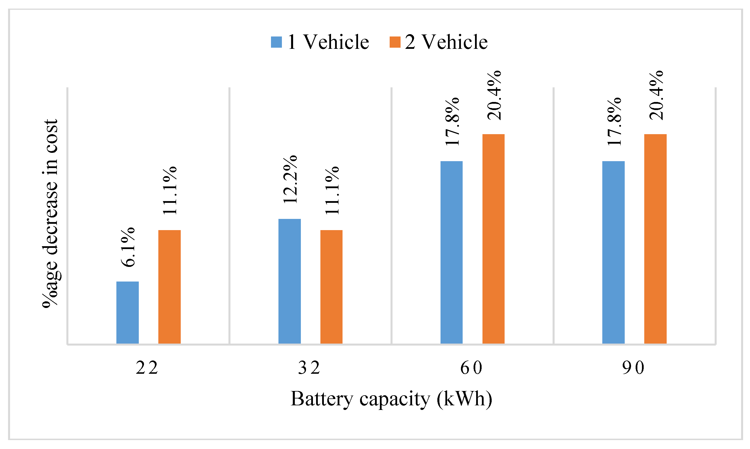
The problem is solved for different battery capacities and the results are presented in Table 13. The enlarged battery capacity enables a BEV to traverse longer trips. Figure 3 shows when the battery capacity is increased from 16 kWh to 60 kWh, the total traveling cost reduces up to 17.8% and 20.4% with one and two operating vehicles, respectively. Moreover, once a minimum number of necessary station visits is achieved, the traveling cost does not reduce with a further increase in battery capacity.
4.3.3. The Bike Carrying Capacity of the BEV (Qk)
A large capacity vehicle can deliver and pick up a large number of bikes from a station. Therefore, the number of visits to a station reduces when the vehicle capacity is increased. Table 14 shows that the traveling distance reduces significantly with an increase in capacity of the vehicle. However, the large-capacity vehicles may add extra operational charges.
4.3.4. The Effect of the Number of Faulty Bikes
The different number of faulty bikes are considered by a 10% drop and increase in the number of faulty bikes. The problem is solved for various percentage presence of faulty or broken bikes within the network and the results are presented in Table 15. The results show that the solutions are not much sensitive to the minor increase or drop in the number of faulty bikes. The total travelling time is changed because of the loading time of the different number of bikes. If the number of faulty bikes at a station exceeds the capacity of the vehicle, these may have a significant effect on the route plan of the rebalancing vehicle. However, this effect will be the same for the ICEV because this is more related to the load carrying capacity of the vehicle rather than the battery capacity constraints. For excessive supply and deliveries, the travelling distances may be longer because of the multiple visits to the stations. Subsequently, the BEV require extra visits to the charging station for battery recharge. This will increase the travelling distances of the BEV as compared to the ICEV as indicated in Table 5. Moreover, the inventory of bikes at the stations will not have a significant effect on the cost comparison of both vehicles because the extra distances travelled by the BEV were already included in the cost–benefit analysis.
5. Discussion and Conclusions
The sharing-bikes dispatching problem is a serious concern towards the sustainability of the bike-sharing systems. Efficient rebalancing operations are the key to ensure good service quality. An inefficient solution for sharing-bikes rebalancing results in wastage of available resources besides a negative impact on the service quality. Therefore, many researchers have focused on optimizing the operational cost. However, the fossil-fueled powered ICEVs were considered for the rebalancing operation. Since BEVs consume less energy than conventional ICEVs, the use of BEVs result in significant energy savings for an urban transport network. However, the routing problem formulation of green vehicles is complex. The conventional formulation does not help to solve the problem with the green vehicles because of the multiple visits to the charging stations.
In this study, we proposed a new model that considers BEVs instead of ICEVs. Using CPLEX solver, the formulated model is demonstrated through various scenarios and the corresponding solutions are presented. The model gives exact solutions for a small-sized problem in few seconds. In addition, to solve larger networks, a clustering-first routing-second approach is presented.
The results show that the BEVs are much better than ICEVs for bike-sharing rebalancing operations because:
- (i)
- The rebalancing operation consists of short-range trips within a small network. Therefore, the BEVs can complete the operation efficiently without excessive visits to the charging station.
- (ii)
- In rebalancing operation, the routing vehicles visit the depot multiple times depending on the demand within the network. The routine visits to the depot can be used to recharge the BEV.
- (iii)
- The high efficiency of the BEVs result in significantly lower operational cost.
While the BEVs need necessary visits to the charging station which increase the total traveling distances besides the operation time, the high energy consumption rate of the ICEVs results in a significantly higher operational cost. The results show that the cost of an ICEV deployed for the same operation is about 14.2 times more as compared to an equivalent BEV.
The major hurdle in adopting the BEVs is their high ownership and charging infrastructure installation cost. For a BEV, the total cost of a charging infrastructure installation is more than the price of the BEV itself and is more than double to the price of an ICEV. Therefore, a detailed cost–benefit analysis of both vehicles is conducted. Besides the high initial cost of BEV, the battery production emission, vehicle manufacturing emission and the indirect emission during electricity production are taken into account in the analysis. The results show that the annual cost incurred on an ICEV is 56.9% more as compared the cost incurred on an equivalent BEV deployed for the operation. In addition, an ICEV has 48.3% more emissions as compared to an equivalent BEV besides taking high battery production and BEV manufacturing emissions into account.
Lastly, the problem is solved in various situations. The results show that the vehicle battery capacity has a significant effect on the routing plan. A vehicle with small battery capacity visits the charging station after a short trip. The extra visits to the charging station not only increase operation cost but also increase the operation time. In addition, excessive battery charging events further delay the operation process. When the battery capacity is increased from 16 kWh to 60 kWh, the total traveling cost reduces up to 17.8% and 20.4% with one and two operating vehicles, respectively. Likewise, the cost of a vehicle with a capacity of 30 bikes is 44% lesser than the cost of the vehicle with a capacity of 15 bikes. Since the BEVs have a high initial cost. Therefore, a detailed cost analysis is required for various capacity vehicles.
The limitations of the presented model are as follows. The travelling speed and battery discharging rate of the BEV is considered as constant. In practice, these are not realistic assumptions. However, the sharing-bikes are usually urban-based services, and a static scenario is assumed for the rebalancing operation. Static rebalancing is performed during the night hours when the system usage is negligible [52]. During night hours, the rebalancing BEV is not subjected to the aggressive acceleration/ deceleration events because of the smooth traffic conditions. Hence, the characteristics of the battery packs of the BEV are less likely to be affected during the static rebalancing operation as compared to the dynamic situations. In addition, the service life of the vehicles in the cost–benefit analysis is considered as 5 years which is less than the service life of the battery packs. In addition, the degradation cost of the battery packs is included in the cost–benefit analysis. Besides, the cost and energy consumption analysis presented in our paper indicates that the BEV consumes considerably lesser energy than an ICEV. The analysis shows that the cost of the ICEV is 53% more than the cost of BEV even if one battery replacement is considered in five-year service life of BEV. Therefore, these assumptions have not a significant impact on the validity of the results.
In fact, taking non-linear speed and battery charging/discharging rate results in a more complex formulation. Consequently, this will result in the non-linear constraints in the model, which are not easy to solve. Therefore, the BEV routing problem might be extended with fewer assumptions in future research. For example, a non-linear battery charging and discharging rates might be considered instead of using constant rates. In addition, efficient solution techniques may be proposed to solve the real-time instances while taking the dynamic situation into account as a part of future research as well.
The presented model gives an exact solution to the small-sized problem. However, the large networks are solved after merging the close satiations through clustering. This may result in an entirely different situation while solving real-time instances. Therefore, in future research, the formation can be extended to solve the large size problem without merging into various clusters. In addition, the solution algorithms might be developed to solve the FFBP with BEVs in a reasonable time.
Lastly, the presented formulations are based on the static demand at each station, i.e., static repositioning. To better synchronize with the real-time scenarios, the models might be extended considering stochastic demand, i.e., dynamic repositioning in the future research as well.
Author Contributions
Y.S. conceived the study idea; M.U. and O.Z. modeled the problem, analyzed the results, and drafted the article; Y.S. revised the article critically for important content.
Funding
This research was supported by the National Natural Science Foundation of China (Grant No. 71701045), and the Fundamental Research Funds for the Central Universities (Grant No. 2242019K40206).
Acknowledgments
The scholarship for authors M.U. and O.Z. graduate studies is provided by China Road and Bridge Corporation (CRBC). I appreciate all the support CRBC offered. The authors would like to thank the anonymous reviewers for their time to review our article and the constructive comments.
Conflicts of Interest
The authors declare no conflict of interest.
References
- Feng, W.; Figliozzi, M. An economic and technological analysis of the key factors affecting the competitiveness of electric commercial vehicles: A case study from the USA market. Transp. Res. Part C Emerg. Technol. 2013, 26, 135–145. [Google Scholar] [CrossRef]
- Conrad, R.G.; Figliozzi, M.A. The Recharging Vehicle Routing Problem. In Proceedings of the Industrial Engineering Research Conference, Reno, NV, USA, 21 May 2011. [Google Scholar]
- Erdoğan, S.; Miller-Hooks, E. A Green Vehicle Routing Problem. Transp. Res. Part E Logist. Transp. Rev. 2012, 48, 100–114. [Google Scholar] [CrossRef]
- Schneider, M.; Stenger, A.; Goeke, D. The Electric Vehicle-Routing Problem with Time Windows and Recharging Stations. Transp. Sci. 2014, 48, 500–520. [Google Scholar] [CrossRef]
- Felipe, Á.; Ortuño, M.T.; Righini, G.; Tirado, G. A heuristic approach for the green vehicle routing problem with multiple technologies and partial recharges. Transp. Res. Part E Logist. Transp. Rev. 2014, 71, 111–128. [Google Scholar] [CrossRef]
- Keskin, M.; Çatay, B. A matheuristic method for the electric vehicle routing problem with time windows and fast chargers. Comput. Oper. Res. 2018, 100, 172–188. [Google Scholar] [CrossRef]
- Goeke, D.; Schneider, M. Routing a mixed fleet of electric and conventional vehicles. Eur. J. Oper. Res. 2015, 245, 81–99. [Google Scholar] [CrossRef]
- Bruglieri, M.; Mancini, S.; Pezzella, F.; Pisacane, O. A new Mathematical Programming Model for the Green Vehicle Routing Problem. Electron. Notes Discret. Math. 2016, 55, 89–92. [Google Scholar] [CrossRef] [Green Version]
- Hiermann, G.; Puchinger, J.; Hartl, R.F. The Electric Fleet Size and Mix Vehicle Routing Problem with Time Windows and Recharging Stations. Eur. J. Oper. Res. 2016, 252, 995–1018. [Google Scholar] [CrossRef] [Green Version]
- Montoya, A.; Guéret, C.; Mendoza, J.E.; Villegas, J.G. The electric vehicle routing problem with nonlinear charging function. Transp. Res. Part B Methodol. 2017, 103, 87–110. [Google Scholar] [CrossRef] [Green Version]
- Lin, J.; Zhou, W.; Wolfson, O. Electric Vehicle Routing Problem. Transp. Res. Procedia 2016, 12, 508–521. [Google Scholar] [CrossRef] [Green Version]
- Desaulniers, G.; Errico, F.; Irnich, S.; Schneider, M. Exact Algorithms for Electric Vehicle-Routing Problems with Time Windows. Oper. Res. 2016, 64, 1388–1405. [Google Scholar] [CrossRef]
- Cairns, S. The Home Delivery of Shopping: The Environmental Consequences; Working Paper for ESRC Transportation Studies Unit; University of Oxford: Oxford, UK, 1999. [Google Scholar]
- Kirby, H.R.; Hutton, B.; McQuaid, R.W.; Raeside, R.; Zhang, X. Modelling the effects of transport policy levers on fuel efficiency and national fuel consumption. Transp. Res. Part D Transp. Environ. 2000, 5, 265–282. [Google Scholar] [CrossRef]
- Palmer, A. The Development of an Integrated Routing and Carbon Dioxide Emissions Model for Goods Vehicles. Ph.D. Thesis, Cranfield University, Cranfield, UK, 2007. [Google Scholar]
- Bektaş, T.; Laporte, G. The Pollution-Routing Problem. Transp. Res. Part B Methodol. 2011, 45, 1232–1250. [Google Scholar] [CrossRef]
- Pan, Y.; Chen, S.; Qiao, F.; Ukkusuri, S.V.; Tang, K. Estimation of real-driving emissions for buses fueled with liquefied natural gas based on gradient boosted regression trees. Sci. Total Environ. 2019, 660, 741–750. [Google Scholar] [CrossRef]
- Zhang, Y.; Jiang, Y.; Rui, W.; Thompson, R.G. Analyzing truck fleets’ acceptance of alternative fuel freight vehicles in China. Renew. Energy 2019, 134, 1148–1155. [Google Scholar] [CrossRef]
- Xiao, Y.; Zhao, Q.; Kaku, I.; Xu, Y. Development of a fuel consumption optimization model for the capacitated vehicle routing problem. Comput. Oper. Res. 2012, 39, 1419–1431. [Google Scholar] [CrossRef]
- Xiao, Y.; Zuo, X.; Kaku, I.; Zhou, S.; Pan, X. Development of energy consumption optimization model for the electric vehicle routing problem with time windows. J. Clean. Prod. 2019, 225, 647–663. [Google Scholar] [CrossRef]
- Ellingsen, L.A.-W.; Hung, C.R.; Strømman, A.H. Identifying key assumptions and differences in life cycle assessment studies of lithium-ion traction batteries with focus on greenhouse gas emissions. Transp. Res. Part D Transp. Environ. 2017, 55, 82–90. [Google Scholar] [CrossRef]
- Médard de Chardon, C.; Caruso, G.; Médard de Chardon, C.; Caruso, G. Transportation Research Part B, Methodological; Elsevier Science: Amsterdam, The Netherlands, 2015; Volume 78. [Google Scholar]
- Jiménez, P.; Nogal, M.; Caulfield, B.; Pilla, F. Perceptually important points of mobility patterns to characterise bike sharing systems: The Dublin case. J. Transp. Geogr. 2016, 54, 228–239. [Google Scholar] [CrossRef]
- Caulfield, B.; O’Mahony, M.; Brazil, W.; Weldon, P. Examining usage patterns of a bike-sharing scheme in a medium sized city. Transp. Res. Part A Policy Pract. 2017, 100, 152–161. [Google Scholar] [CrossRef]
- Ji, Y.; Fan, Y.; Ermagun, A.; Cao, X.; Wang, W.; Das, K. Public bicycle as a feeder mode to rail transit in China: The role of gender, age, income, trip purpose, and bicycle theft experience. Int. J. Sustain. Transp. 2017, 11, 308–317. [Google Scholar] [CrossRef]
- Chen, J.; Li, Z.; Wang, W.; Jiang, H. Evaluating bicycle–vehicle conflicts and delays on urban streets with bike lane and on-street parking. Transp. Lett. 2018, 10, 1–11. [Google Scholar] [CrossRef]
- Guo, Y.; Li, Z.; Wu, Y.; Xu, C. Evaluating factors affecting electric bike users’ registration of license plate in China using Bayesian approach. Transp. Res. Part F Traffic Psychol. Behav. 2018, 59, 212–221. [Google Scholar] [CrossRef]
- Ji, Y.; Ma, X.; Yang, M.; Jin, Y.; Gao, L. Exploring Spatially Varying Influences on Metro-Bikeshare Transfer: A Geographically Weighted Poisson Regression Approach. Sustainability 2018, 10, 1526. [Google Scholar] [CrossRef]
- Wang, C.; Xu, C.; Xia, J.; Qian, Z. Modeling faults among e-bike-related fatal crashes in China. Traffic Inj. Prev. 2017, 18, 175–181. [Google Scholar] [CrossRef] [PubMed]
- Du, M.; Cheng, L. Better Understanding the Characteristics and Influential Factors of Different Travel Patterns in Free-Floating Bike Sharing: Evidence from Nanjing, China. Sustainability 2018, 10, 1244. [Google Scholar] [CrossRef]
- Fu, X.; Lam, W.H.K. Modelling joint activity-travel pattern scheduling problem in multi-modal transit networks. Transportation 2018, 45, 23–49. [Google Scholar] [CrossRef]
- Zhang, Y.; Brussel, M.J.G.; Thomas, T.; van Maarseveen, M.F.A.M. Mining bike-sharing travel behavior data: An investigation into trip chains and transition activities. Comput. Environ. Urban Syst. 2018, 69, 39–50. [Google Scholar] [CrossRef]
- Biehl, A.; Ermagun, A.; Stathopoulos, A. Community mobility MAUP-ing: A socio-spatial investigation of bikeshare demand in Chicago. J. Transp. Geogr. 2018, 66, 80–90. [Google Scholar] [CrossRef]
- Borgnat, P.; Robardet, C.; Rouquier, J.-B.; Abry, P.; Fleury, E.; Flandrin, P.; Borgnat, P.; Abry, P.; Flandrin, P.; Rouquier, J.-B.; et al. Shared Bicycles in a City: A Signal Processing and Data Analysis Perspective. Adv. Complex Syst. 2010, 14, 415–438. [Google Scholar] [CrossRef]
- Corcoran, J.; Li, T.; Rohde, D.; Charles-Edwards, E.; Mateo-Babiano, D. Spatio-temporal patterns of a Public Bicycle Sharing Program: The effect of weather and calendar events. J. Transp. Geogr. 2014, 41, 292–305. [Google Scholar] [CrossRef]
- Montoliu, R. Discovering Mobility Patterns on Bicycle-Based Public Transportation System by Using Probabilistic Topic Models; Springer: Berlin/Heidelberg, Germany, 2012; pp. 145–153. [Google Scholar]
- Sarkar, A.; Lathia, N.; Mascolo, C. Comparing cities’ cycling patterns using online shared bicycle maps. Transportation 2015, 42, 541–559. [Google Scholar] [CrossRef]
- Vogel, P.; Greiser, T.; Mattfeld, D.C. Understanding Bike-Sharing Systems using Data Mining: Exploring Activity Patterns. Procedia Soc. Behav. Sci. 2011, 20, 514–523. [Google Scholar] [CrossRef] [Green Version]
- Guo, Y.; Li, Z.; Wu, Y.; Xu, C. Exploring unobserved heterogeneity in bicyclists’ red-light running behaviors at different crossing facilities. Accid. Anal. Prev. 2018, 115, 118–127. [Google Scholar] [CrossRef] [PubMed]
- Benchimol, M.; Benchimol, P.; Chappert, B.; de la Taille, A.; Laroche, F.; Meunier, F.; Robinet, L. Balancing the stations of a self service “bike hire” system. RAIRO Oper. Res. 2011, 45, 37–61. [Google Scholar] [CrossRef]
- Chemla, D.; Meunier, F.; Wolfler Calvo, R. Bike sharing systems: Solving the static rebalancing problem. Discret. Optim. 2013, 10, 120–146. [Google Scholar] [CrossRef]
- Erdoğan, G.; Laporte, G.; Wolfler Calvo, R. The static bicycle relocation problem with demand intervals. Eur. J. Oper. Res. 2014, 238, 451–457. [Google Scholar] [CrossRef] [Green Version]
- Contardo, C.; Rousseau, L.-M.; Morency, C. Balancing a Dynamic Public Bike-Sharing System; Cirrelt: Montreal, QC, Canada, 2012; Volume 4. [Google Scholar]
- Raviv, T.; Tzur, M.; Forma, I.A. Static repositioning in a bike-sharing system: Models and solution approaches. Eur. J. Transp. Logist. 2013, 2, 187–229. [Google Scholar] [CrossRef]
- Schuijbroek, J.; Hampshire, R.; van Hoeve, W.-J. Inventory Rebalancing and Vehicle Routing in Bike Sharing Systems Inventory Rebalancing and Vehicle Routing in Bike Sharing Systems. Eur. J. Oper. Res. 2017, 257, 992–1004. [Google Scholar] [CrossRef]
- Pal, A.; Zhang, Y. Free-floating bike sharing: Solving real-life large-scale static rebalancing problems. Transp. Res. Part C Emerg. Technol. 2017, 80, 92–116. [Google Scholar] [CrossRef]
- Liu, Y.; Szeto, W.Y.; Ho, S.C. A static free-floating bike repositioning problem with multiple heterogeneous vehicles, multiple depots, and multiple visits. Transp. Res. Part C Emerg. Technol. 2018, 92, 208–242. [Google Scholar] [CrossRef]
- Sebastian, I.; Christoph, N. The Evolution of Free-Floating Bike-Sharing in China. Available online: http://www.sustainabletransport.org/archives/6278 (accessed on 15 May 2019).
- Hui, Z. Beijing Puts Brakes on E-bike Sharing, Restricts Total Number of For-Hire Bikes. Available online: http://www.globaltimes.cn/content/1066602.shtml (accessed on 15 May 2019).
- Yin, J.; Qian, L.; Shen, J. From value co-creation to value co-destruction? The case of dockless bike sharing in China. Transp. Res. Part D Transp. Environ. 2019, 79, 169–185. [Google Scholar] [CrossRef]
- Alvarez-Valdes, R.; Belenguer, J.M.; Benavent, E.; Bermudez, J.D.; Muñoz, F.; Vercher, E.; Verdejo, F. Optimizing the level of service quality of a bike-sharing system. Omega 2016, 62, 163–175. [Google Scholar] [CrossRef]
- Wang, Y.; Szeto, W.Y. Static green repositioning in bike sharing systems with broken bikes. Transp. Res. Part D Transp. Environ. 2018, 65, 438–457. [Google Scholar] [CrossRef]
- Usama, M.; Shen, Y.; Zahoor, O. A free-floating bike repositioning problem with faulty bikes. Procedia Comput. Sci. 2019, 151, 155–162. [Google Scholar] [CrossRef]
- Dell’Amico, M.; Hadjicostantinou, E.; Iori, M.; Novellani, S. The bike sharing rebalancing problem: Mathematical formulations and benchmark instances. Omega 2014, 45, 7–19. [Google Scholar] [CrossRef]
- Ho, S.C.; Szeto, W.Y. Solving a static repositioning problem in bike-sharing systems using iterated tabu search. Transp. Res. Part E Logist. Transp. Rev. 2014, 69, 180–198. [Google Scholar] [CrossRef] [Green Version]
- Zhang, S.; Xiang, G.; Huang, Z. Bike-Sharing Static Rebalancing by Considering the Collection of Bicycles in Need of Repair. J. Adv. Transp. 2018, 2018, 1–18. [Google Scholar] [CrossRef]
- Genta, G. Motor Vehicle Dynamics: Modeling and Simulation; Series on Advances in Mathematics for Applied Sciences; World Scientific: Singapore, 1997; Volume 43, ISBN 978-981-02-2911-5. [Google Scholar]
- Akcelik, R.; Besley, M. Operating cost, fuel consumption, and emission models in aaSIDRA and aaMOTION. In Proceedings of the 25th Conference of Australian Institutes of Transport Research, Adelaide, Australia, 3–5 December 2003. [Google Scholar]
- Bureau of Labor Statistics. Average Energy Prices, New York-Newark-Jersey City-February; Bureau of Labor Statistics: Washington, DC, USA, 2019.
- BU-1003: Electric Vehicle (EV)—Battery University. Available online: https://batteryuniversity.com/learn/article/electric_vehicle_ev (accessed on 18 May 2019).
- Ubeda, S.; Arcelus, F.J.; Faulin, J. Green logistics at Eroski: A case study. Int. J. Prod. Econ. 2011, 131, 44–51. [Google Scholar] [CrossRef]
- Zhang, S.; Lee, C.K.M.; Choy, K.L.; Ho, W.; Ip, W.H. Design and development of a hybrid artificial bee colony algorithm for the environmental vehicle routing problem. Transp. Res. Part D Transp. Environ. 2014, 31, 85–99. [Google Scholar] [CrossRef] [Green Version]
- Pelletier, S.; Jabali, O.; Laporte, G.; Veneroni, M. Battery degradation and behaviour for electric vehicles: Review and numerical analyses of several models. Transp. Res. Part B Methodol. 2017, 103, 158–187. [Google Scholar] [CrossRef]
- Sarasketa-Zabala, E.; Laresgoiti, I.; Alava, I.; Rivas, M.; Villarreal, I.; Blanco, F. Validation of the methodology for lithium-ion batteries lifetime prognosis. In Proceedings of the 2013 World Electric Vehicle Symposium and Exhibition, Barcelona, Spain, 17–20 November 2013. [Google Scholar]
- Jabali, O.; Van Woensel, T.; de Kok, A.G. Analysis of Travel Times and CO2 Emissions in Time-Dependent Vehicle Routing. Prod. Oper. Manag. 2012, 21, 1060–1074. [Google Scholar] [CrossRef]
- John, W.B.; Timothy, E.B. Battery Electric Vehicles vs. Internal Combustion Engine Vehicles. A United States-Based Comprehensive Assessment. Available online: http://www.adlittle.cn/sites/default/files/viewpoints/ADL_BEVs_vs_ICEVs_FINAL_November_292016.pdf (accessed on 7 September 2017).
- Earl, T.; Mathieu, L.; Cornelis, S.; Kenny, S.; Ambel, C.C.; Nix, J. Analysis of long haul battery electric trucks in EU Marketplace and Technology, Economic, Environmental, and Policy Perspectives. In Proceedings of the 8th Commercial Vehicle Workshop, Graz, Austrian, 17–18 May 2018. [Google Scholar]
- Kim, H.C.; Wallington, T.J.; Arsenault, R.; Bae, C.; Ahn, S.; Lee, J. Cradle-to-Gate Emissions from a Commercial Electric Vehicle Li-Ion Battery: A Comparative Analysis. Environ. Sci. Technol. 2016, 50, 7715–7722. [Google Scholar] [CrossRef] [PubMed]
Figure 1.
The location of a depot and stations in a bike-sharing scheme.
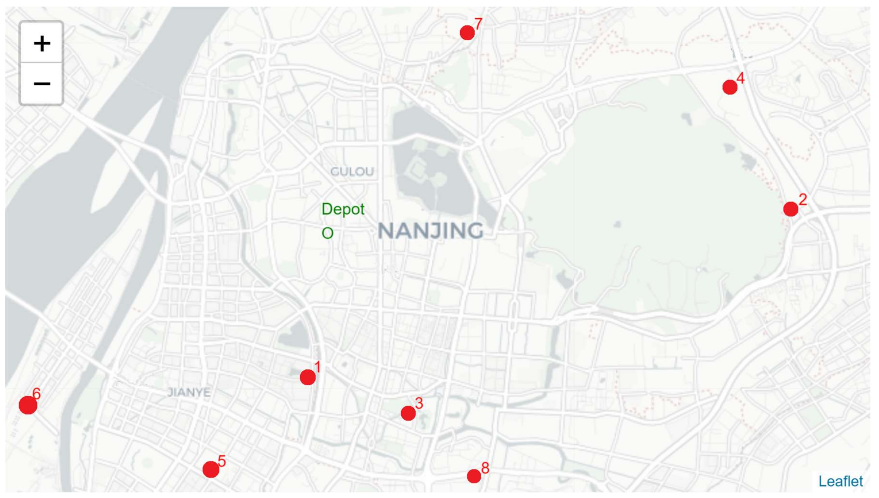
Figure 2.
Bike-sharing network with 50 stations and their cluster centroids.
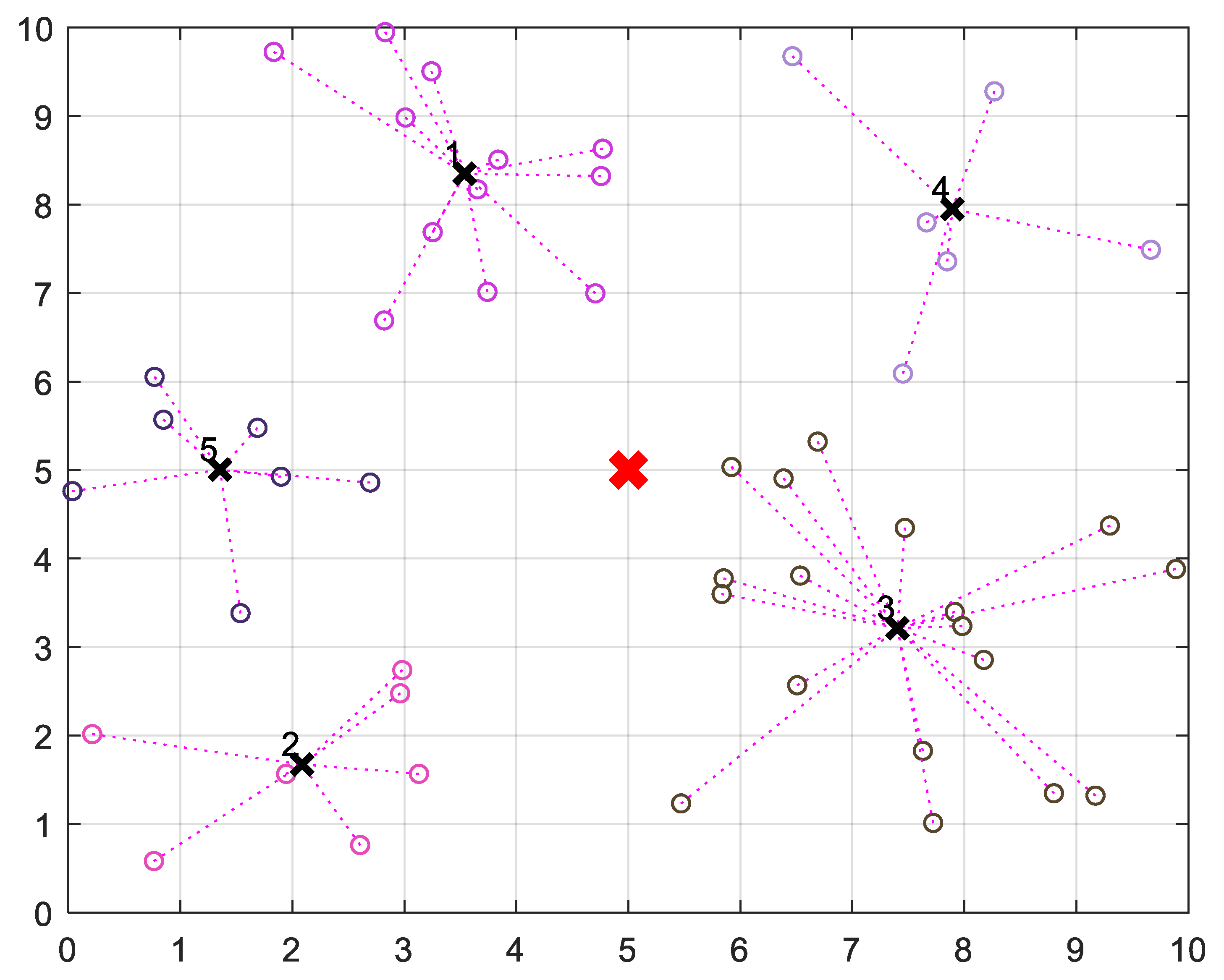
Figure 3.
Percentage decrease in total traveling cost under different battery capacities.

Table 1.
Summary of the characteristics of the static rebalancing problems in the literature.
| Reference | FFBS | DBS | Multiple Vehicles | Multiple Visits | Faulty Bikes | EI | BEV | EC |
|---|---|---|---|---|---|---|---|---|
| Benchimol et al., (2011) [40] | ✓ | |||||||
| Chemla et al., (2013) [41] | ✓ | ✓ | ||||||
| Dell’Amico et al., (2014) [54] | ✓ | ✓ | ||||||
| Ho and Szeto, (2014) [55] | ✓ | |||||||
| Alvarez-Valdes et al., (2016) [51] | ✓ | ✓ | ✓ | ✓ | ||||
| Liu et al., (2018) [47] | ✓ | ✓ | ||||||
| Pal and Zhang (2017) [46] | ✓ | ✓ | ||||||
| Zhang et al., (2018) [56] | ✓ | ✓ | ✓ | |||||
| Wang and Szeto, (2018) [52] | ✓ | ✓ | ✓ | ✓ | ||||
| Usama et al., (2019) [53] | ✓ | ✓ | ✓ | |||||
| This Study | ✓ | ✓ | ✓ | ✓ | ✓ | ✓ | ✓ |
EI: environmental issue; BEV: battery electric vehicle; EC: Energy consumption; DBS: Docked bike-sharing system.
Table 2.
Parameter values used for estimating energy consumption and emission rates.
| Parameter | Description | Values | Reference |
|---|---|---|---|
| A | The frontal surface area of the vehicle (m2) | 5 | [16] |
| ρ | Air density (kg/m3) | 1.2041 | [57] |
| v | Vehicle speed (km/h) | 40 | [16] |
| Cd | Coefficient of rolling drag | 0.7 | [58] |
| θ | Road angle (degrees) | 0° | [57] |
| Cr | Coefficient of rolling resistance | 0.01 | [57] |
| W | Empty vehicle weight (tons) | 3.629 | [11] |
| g | Gravitational constant (m/s2) | 9.81 | |
| cf | Diesel price ($/L) | 1.309 | [59] |
| ce | Battery charging cost ($/kWh) | 0.136 | [59] |
| ϕ | Additional Energy consumed for one unit of load on a BEV for a vehicle with capacity 200 units | 1.6 × 10⁻⁶ | [20] |
| r | EV battery charging rate (kW) | 22 | [60] |
| CER | CO2 emission rate (kg/L) | 2.61 | [61] |
| ρ* | Full load fuel consumption rate (L/km) | 0.39 | [61] |
| ρo | Empty load fuel consumption rate (L/km) | 0.296 | [61] |
Table 3.
The number of present usable and faulty bikes, and the next day demand at each station.
| Station | Present Inventory | Next Day Demand Interval | Minimum Shortage of Bikes | Maximum Supply of Bikes | Faulty Bikes |
|---|---|---|---|---|---|
| O | N | - | - | ||
| 1 | 30 | [35, 44] | 05 | - | 1 |
| 2 | 10 | [02, 03] | - | 08 | 1 |
| 3 | 10 | [17, 23] | 07 | - | 0 |
| 4 | 35 | [05, 13] | - | 30 | 3 |
| 5 | 40 | [20, 28] | - | 20 | 0 |
| 6 | 25 | [47, 53] | 22 | - | 0 |
| 7 | 20 | [26, 33] | 06 | - | 1 |
| 8 | 20 | [27, 33] | 07 | - | 0 |
| Total | 190 | [179, 230] | 47 | 58 | 6 |
Table 4.
The shortest travel distances in kilometers (km) between each station retrieved from OpenStreetMap using Python 3.7.
Table 4.
The shortest travel distances in kilometers (km) between each station retrieved from OpenStreetMap using Python 3.7.
| Station | O | 1 | 2 | 3 | 4 | 5 | 6 | 7 | 8 |
|---|---|---|---|---|---|---|---|---|---|
| O | 0 | 5 | 15 | 6 | 19 | 8 | 11 | 7 | 9 |
| 1 | 5 | 0 | 18 | 3 | 18 | 4 | 9 | 11 | 6 |
| 2 | 15 | 18 | 0 | 13 | 6 | 18 | 22 | 12 | 13 |
| 3 | 6 | 3 | 13 | 0 | 17 | 6 | 11 | 10 | 3 |
| 4 | 19 | 18 | 6 | 17 | 0 | 19 | 22 | 8 | 15 |
| 5 | 8 | 4 | 18 | 6 | 19 | 0 | 7 | 15 | 7 |
| 6 | 11 | 9 | 22 | 11 | 22 | 7 | 0 | 17 | 12 |
| 7 | 7 | 11 | 12 | 10 | 8 | 15 | 17 | 0 | 11 |
| 8 | 9 | 6 | 13 | 3 | 15 | 7 | 12 | 11 | 0 |
Table 5.
Optimal solutions for electric and conventional vehicles.
| Experiment | Charging Rate (kW) | Battery Capacity | Vehicle Type | Vehicles | Trips | Route | Vehicle Load | Stops | Vehicles Operation Time (min) | Distance Travelled (km) | Battery State of Charging (SoC) kWh |
|---|---|---|---|---|---|---|---|---|---|---|---|
| 1 | 22 | 16 | BEV | 1 | 2 | 0-2-4-8-3-1-0 | 0-8-20-13-6-2 | 13 | 271 | 109 | 14.4-11.4-10.2-7.2-6.6-6 |
| 0-7-4-6-5-6-0 | 6-1-14-8-20-4 | 14.4-13-11.4-7-5.6-4.2-2 | |||||||||
| 2 | - | - | ICEV | 1 | 1 | 0-7-4-8-3-2-4-6-5-6-1-0 | 6-1-15-8-1-9-20-8-20-10-10-6 | 12 | 260 | 102 | - |
Table 6.
Energy consumption and routing cost of the battery electric vehicle (BEV).
| Station | Routing Cost ($) | ||||
|---|---|---|---|---|---|
| From, i | To, j | ||||
| 0 | 2 | 15 | 0 | 3.00 | 0.41 |
| 2 | 4 | 6 | 8 | 1.27 | 0.17 |
| 4 | 8 | 15 | 20 | 3.41 | 0.46 |
| 8 | 3 | 3 | 13 | 0.65 | 0.09 |
| 3 | 1 | 3 | 6 | 0.62 | 0.08 |
| 1 | 0 | 5 | 2 | 1.01 | 0.14 |
| 0 | 7 | 7 | 6 | 1.46 | 0.20 |
| 7 | 4 | 8 | 1 | 1.61 | 0.22 |
| 4 | 6 | 22 | 14 | 4.82 | 0.66 |
| 6 | 5 | 7 | 8 | 1.48 | 0.20 |
| 5 | 6 | 7 | 20 | 1.59 | 0.22 |
| 6 | 0 | 11 | 4 | 2.26 | 0.31 |
| Total | 109 km | - | 23.2 kWh | $3.2 | |
Table 7.
The fuel consumption rate, fuel cost and the emission of the conventional vehicle for the rebalancing operation.
Table 7.
The fuel consumption rate, fuel cost and the emission of the conventional vehicle for the rebalancing operation.
| Station | FCR (L/km) | Fuel Consumption (L) | Emissions (kg) | ||||
|---|---|---|---|---|---|---|---|
| From, i | To, j | ||||||
| 0 | 7 | 7 | 6 | 0.32 | 2.27 | 2.97 | 5.92 |
| 7 | 4 | 8 | 1 | 0.30 | 2.41 | 3.15 | 6.28 |
| 4 | 8 | 15 | 15 | 0.37 | 5.50 | 7.20 | 14.35 |
| 8 | 3 | 3 | 8 | 0.33 | 1.00 | 1.31 | 2.61 |
| 3 | 2 | 13 | 1 | 0.30 | 3.91 | 5.12 | 10.20 |
| 2 | 4 | 6 | 9 | 0.34 | 2.03 | 2.66 | 5.30 |
| 4 | 6 | 22 | 20 | 0.39 | 8.58 | 11.23 | 22.39 |
| 6 | 5 | 7 | 8 | 0.33 | 2.34 | 3.06 | 6.09 |
| 5 | 6 | 7 | 20 | 0.39 | 2.73 | 3.57 | 7.13 |
| 6 | 1 | 9 | 10 | 0.34 | 3.09 | 4.04 | 8.06 |
| 1 | 0 | 5 | 6 | 0.32 | 1.62 | 2.12 | 4.23 |
| Total | 102 km | 35.5 L | $46.4 | 92.6 kg | |||
Table 8.
Life cycle cost assessment of BEVs and internal combustion engine vehicles (ICEVs).
| Cost | BEV | ICEV | Source |
|---|---|---|---|
| Purchase Cost ($) | 37,900 | 19,100 | [66] |
| Charging infrastructure | 40,000 | 0 | [67] |
| Battery degradation cost ($) | 1280 | 0 | |
| Maintenance cost per annum ($) | 7000 | 14,000 | [67] |
| Battery production emissions cost ($) | 83.95 | 0 | [65,67] |
| Vehicle manufacturing process emissions cost ($) | 82.6 | 73 | [65,66] |
| Operational Cost($) per annum | 2143 | 32,207 | Table 6, Table 71 |
| Cost of emissions during operation per annum ($) | - | 816.5 | Table 6, Table 71 |
| Indirect emission cost per annum ($) | 396.6 | [67] |
1 The results are used to estimate operation and emissions cost for annual 74,000 km distance travelled.
Table 9.
The annual cost–benefit analysis of BEV and ICEV.
| Cost per Annum | BEV | ICEV |
|---|---|---|
| Purchase cost | $7580.00 | $3820.00 |
| Infrastructure cost | $8000.00 | $0.00 |
| Battery degradation cost | $256 | |
| Maintenance cost | $7000.00 | $14,000.00 |
| Annual operational Cost | $3650.00 | $32,850.00 |
| Direct and indirect Emission cost | $396.62 | $816.40 |
| Battery emission cost | $16.79 | $0.00 |
| Manufacturing emissions cost | $16.51 | $14.59 |
| Depreciation cost | −$3895.00 | −$955.00 |
| Total Cost per annum | $21,513.91 | $49,903.87 |
Table 10.
The number of present usable and faulty bikes, and the next day demand at each cluster.
| Cluster | Present Inventory | Next Day Demand | Bike Deficiency | Bike Excess | Faulty Bikes |
|---|---|---|---|---|---|
| 1 | 155 | [210, 230] | 55 | 0 | 3 |
| 2 | 200 | [140 165] | 0 | 35 | 1 |
| 3 | 250 | [180 220] | 0 | 30 | 3 |
| 4 | 100 | [50, 65] | 0 | 35 | 2 |
| 5 | 50 | [105, 110] | 55 | 0 | 4 |
| Total | 755 | 110 | 100 | 13 |
Table 11.
Travel distances (km) from the cluster centroids.
| Zone | O | 1 | 2 | 3 | 4 | 5 |
|---|---|---|---|---|---|---|
| O | 0 | 20.5 | 21.6 | 19.5 | 21.2 | 20.5 |
| 1 | 20.5 | 0 | 25.2 | 24.6 | 21.6 | 21.0 |
| 2 | 21.6 | 25.2 | 0 | 23.3 | 27.8 | 20.1 |
| 3 | 19.5 | 24.6 | 23.3 | 0 | 22.1 | 24.5 |
| 4 | 21.2 | 21.6 | 27.8 | 22.1 | 0 | 25.8 |
| 5 | 20.5 | 21.0 | 20.1 | 24.5 | 25.8 | 0 |
Table 12.
The optimal solutions under different numbers of vehicles used for the rebalancing operation.
Table 12.
The optimal solutions under different numbers of vehicles used for the rebalancing operation.
| No. of Vehicles | Battery Capacity (kWh) | Vehicle Capacity (Qk) | Trips | Stops | Total Travelling Distance (km) | Total Travelling Time (min) | Optimality Gap (%) | CPU Time (s) |
|---|---|---|---|---|---|---|---|---|
| 1 | 16 | 20 | 5 | 18 | 359.9 | 785.5 | 0.01 | 665.8 |
| 2 | 16 | 20 | 8 | 20 | 380.1 | 816.5 | 0.01 | 171.3 |
| 3 | 16 | 20 | 9 | 21 | 380.1 | 816.15 | 5.05 | 11.17 |
Table 13.
The optimal solutions under different Battery capacities of the BEV (qk).
| No. of Vehicles | Battery Capacity (kWh) | Vehicle Capacity (Q) | Trips | Stops | Total Travelling Distance (km) | Total Travelling Time (min) | Optimality Gap (%) | CPU Time (s) |
|---|---|---|---|---|---|---|---|---|
| 1 | 22 | 20 | 4 | 17 | 337.9 | 752.85 | 0.01 | 532.7 |
| 1 | 32 | 20 | 3 | 16 | 316 | 720 | 0.01 | 285.25 |
| 1 | 60 | 20 | 2 | 15 | 295.8 | 689.7 | 0.01 | 48.69 |
| 1 | 90 | 20 | 2 | 15 | 295.8 | 689.7 | 0.01 | 45.7 |
| 2 | 22 | 20 | 6 | 18 | 337.9 | 752.85 | 0.01 | 45.7 |
| 2 | 32 | 20 | 6 | 18 | 337.9 | 752.85 | 0.01 | 314.43 |
| 2 | 60 | 20 | 2 | 16 | 302.4 | 699.6 | 0.01 | 2.25 |
| 2 | 90 | 20 | 2 | 16 | 302.4 | 699.6 | 0.01 | 1.66 |
Table 14.
The optimal solutions under different vehicle capacities (Qk).
| No. of Vehicles | Battery Capacity (kWh) | Vehicle Capacity (Q) | Trips | Stops | Travelling Distance (km) | Traveling Time (min) | Optimality Gap (%) | CPU Time (s) |
|---|---|---|---|---|---|---|---|---|
| 1 | 16 | 15 | 8 | 26 | 524.2 | 1032.3 | 1.3 | 1200 |
| 1 | 16 | 25 | 5 | 18 | 355 | 778.5 | 1 | 1200 |
| 1 | 16 | 30 | 4 | 15 | 292.2 | 684.9 | 0.01 | 56.5 |
| 2 | 16 | 15 | 4 | 14 | 543.2 | 1060.8 | 1 | 1200 |
| 4 | 14 | |||||||
| 2 | 16 | 25 | 3 | 10 | 377.1 | 811.65 | 0.01 | 238.6 |
| 3 | 10 | |||||||
| 2 | 16 | 30 | 2 | 8 | 292.6 | 684.9 | 0.01 | 17.91 |
| 2 | 8 |
Table 15.
The optimal solutions under different numbers of faulty bikes in the network.
| No. of Vehicles | Faulty Bikes | Battery Capacity (kWh) | Trips | Stops | Total Travelling Distance (km) | Total Travelling Time (min) |
|---|---|---|---|---|---|---|
| 1 | 13 | 16 | 5 | 18 | 359.9 | 785.5 |
| 1 | 11 (−10%) | 16 | 5 | 18 | 359.9 | 781.9 |
| 1 | 15 (+10%) | 16 | 5 | 18 | 359.9 | 789.9 |
© 2019 by the authors. Licensee MDPI, Basel, Switzerland. This article is an open access article distributed under the terms and conditions of the Creative Commons Attribution (CC BY) license (http://creativecommons.org/licenses/by/4.0/).
Share and Cite
MDPI and ACS Style
Usama, M.; Shen, Y.; Zahoor, O. Towards an Energy Efficient Solution for Bike-Sharing Rebalancing Problems: A Battery Electric Vehicle Scenario. Energies 2019, 12, 2503. https://doi.org/10.3390/en12132503
AMA Style
Usama M, Shen Y, Zahoor O. Towards an Energy Efficient Solution for Bike-Sharing Rebalancing Problems: A Battery Electric Vehicle Scenario. Energies. 2019; 12(13):2503. https://doi.org/10.3390/en12132503
Chicago/Turabian StyleUsama, Muhammad, Yongjun Shen, and Onaira Zahoor. 2019. "Towards an Energy Efficient Solution for Bike-Sharing Rebalancing Problems: A Battery Electric Vehicle Scenario" Energies 12, no. 13: 2503. https://doi.org/10.3390/en12132503
Note that from the first issue of 2016, this journal uses article numbers instead of page numbers. See further details here.