Optimal Economic Dispatch for Integrated Power and Heating Systems Considering Transmission Losses

Abstract

To address the problem of the supply–demand imbalance caused by network transmission losses in integrated power and heating systems (IPHS), this paper presents an optimal economic dispatch strategy to minimize system operation cost and realize coordination and optimization between power and heat. Firstly, an innovative economic dispatch model considering transmission losses is developed, where both power and heat transmission losses models are established with good precision together. In addition, the coordination equation is derived from the formulated nonlinear, multi-constrained coupling optimization problem, where the coordination relationship of units’ outputs is clearly analyzed in an analytic way. Then, a double-$\lambda$-iteration algorithm is proposed, which can not only effectively solve the nonlinear coupling optimization problem but also decrease computation burden with faster convergence rate. Finally, simulations performed on five case studies illustrate the satisfying performance of the presented strategy.

1. Introduction

As a core part of integrated energy systems [1,2,3], IPHS refer to the organic coordination and optimization of electric energy and heat energy in the process of planning, construction and operation, where production, transmission, distribution, conversion, storage and consumption have been performed holistically. With coupling elements such as combined heat and power (CHP) [4,5,6] units being integrated, the originally independent power system and heating system can be coupled closely in IPHS. By this way, IPHS can not only achieve diversified energy supply and efficient energy conversion but also ensure energy supply to be sustainable and reliable.

Technologies related to IPHS have been highly valued by researchers and technicians in the global energy field [7,8,9,10]. At present, relevant research has mainly focused on promoting the application of distributed energies and cogeneration technologies, increasing the use proportion of renewable energy resources, and advancing collaborative optimization among multiple energy resources, etc. The work studied in this paper will focus on the economic dispatch of IPHS, which aims at minimizing the total system operation cost for power and heat generation of multiple units, while meeting users’ actual energy demands and scheduling units’ optimal outputs.

The economic dispatch problem (EDP) is one of the most important optimization problems of power system operation, which aims at minimizing the total operation cost while satisfying both system-level and unit-level constraints [11]. The EDP can be typically formulated as a constrained optimization problem, and existing solving algorithms for economic dispatch can be classified into two categories: analytic optimization algorithms such as iteration method [12], Newton’s method [13], linear programming method [14], and heuristic optimization algorithms such as genetic algorithm [15], particle swarm optimization [16], and bee colony optimization [17]. It can be noted that EDP of power systems considering power transmission losses has been studied well [11], and there have been many methods to handle the EDP. However, the EDP of power systems is only the study of the single power optimization dispatch, which cannot realize collaborative optimization and economic distribution among multiple energy resources, and it cannot meet the developing trend of the future power grid to integrated energy systems with diversified energy supply and consumption.

Extending this issue to IPHS, domestic and foreign scholars have done some noticeable research. The authors in [18] have proposed a classical CHP economic dispatch model. In addition, the authors in [19] have developed a day-ahead economic dispatch model for regional IPHS to comprehensively consider the wind curtailment cost, electric vehicle dispatch cost and so on. The authors in [20] have presented a holistic optimization dispatching method to minimize the operation cost of the integrated community energy system. However, none of them have considered transmission losses. With power transmission losses, the authors in [21] have designed a line-up competition algorithm and the authors in [22] have proposed an optimization technique based on time-varying acceleration particle swarm optimization to handle CHP multi-objective optimization problems, but neither of them have considered heat transmission losses and network transmission constraints. Defining power and heat losses coefficients, the authors in [23] have presented a distributed neurodynamic-based approach to solve the EDP of integrated energy systems, but neither power nor heat transmission losses model have been established, which means that both of them have been simply considered as constants to a certain extent.

At present, the EDP of IPHS considering network transmission losses is a relatively novel but complex problem, and there have hardly been good model combinations to estimate both power and heat transmission losses at the same time. In other words, the EDP discussed in most of the existing literature is based on the ideal conditions without network transmission losses. Although the goal of economic dispatch has been achieved through reasonable allocations, the optimal solutions are accompanied by many problems due to the existences of transmission losses. On one hand, due to neglecting power transmission losses, it is easy to cause supply–demand imbalance [21,24] and suboptimal solutions [25,26], which cannot meet users’ actual load demands well. On the other hand, due to neglecting heat transmission losses, it is easy to cause insufficient heat supply, which will damage users’ experiences and even bring serious economic losses [7].

To address the above problems, this paper has studied the optimal economic dispatch of IPHS with network transmission losses, and our major contributions of this paper can be given as follows:

• A novel economic dispatch model is developed for IPHS with network transmission losses, where both power and heat transmission losses are considered with good precision together, and network transmission constraints are extra considered for the practical application significance. In addition, supply–demand equality constraints and output inequality constraints are routinely considered.
• By constructing the systemic Lagrangian function, the coordination equation is derived from the formulated nonlinear, multi-constrained coupling optimization problem, where the coordination relationship of units’ outputs is clearly analyzed, and the optimal solutions are illustrated in an analytic way considering output inequality constraints.
• A double-$\lambda$-iteration algorithm is proposed to effectively solve this innovative EDP, which can not only decrease computation burden but also protect the privacy of power-heat subsystems to a large extent. More importantly, it can provide optimal analytic solutions with faster convergence rate than heuristic optimization algorithms.
• The total cost of power and heat generation is minimized while ensuring the supply–demand balance, and all of the units’ outputs are optimized to relieve the transmission line and pipeline congestions. Moreover, simulations performed on five case studies illustrate the satisfying performance of the presented approach.

The rest of this paper is organized as follows: Section 2 introduces some basics on IPHS. Section 3 develops a novel economic dispatch model with network transmission losses. Section 4 analyzes the coordination relationship of units’ outputs. Section 5 proposes a double-$\lambda$-iteration algorithm. Section 6 shows the simulation results of the presented method, and conclusions and perspectives for future works are given in Section 7.

2. Integrated Power and Heating Systems

Traditional power systems and heating systems simply optimize for the single energy form of electric energy or heat energy, which cannot achieve complementary advantages and collaborative benefits between energy resources. Relying on advanced communication and control technologies, IPHS can realize mutual coordinations among electric energy, heat energy, energy storage and load through the optimization dispatch, and it can also construct a cost-effective, eco-friendly and flexible way with the integration of production, supply and consumption.

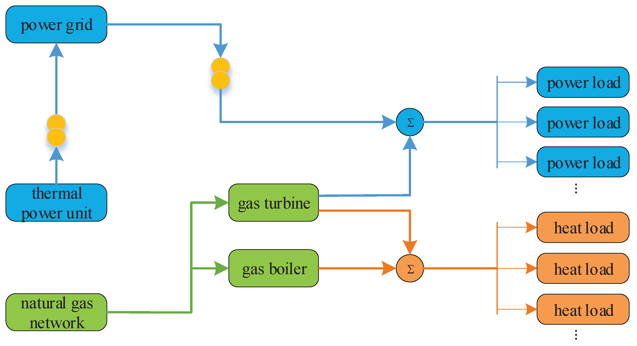
Generalized IPHS involve the production, transmission, distribution, consumption and other aspects of electric energy and heat energy, so it is very complex to carry out research on its whole. At present, scholars mainly start from narrow IPHS. By developing a novel economic dispatch model with network transmission losses, this paper further reduces the imbalance between supply-side and demand-side caused by transmission losses, while meeting users’ energy demands and minimizing the enterprises’ production cost. The structure diagram of the IPHS studied in this paper is shown in Figure 1, which can be mainly used in industrial parks, intelligent factories, intelligent buildings, etc.

Notice that there is no consideration of energy storage units in Figure 1; the reasons can be attributed to two aspects. First, energy storage units are mainly used to stabilize the fluctuations of intermittent renewable energy resources, which should be considered as a whole rather than as a separate part if necessary. Second, for the EDP of IPHS studied in this paper, it can be classified into the single-period economic dispatch field such as [12,22,23,25], which aims at guiding the supply-side to develop an optimal generation scheme and dispatching different units to arrange a reasonable output plan. However, for ensuring the balance constraint between initial state of charge (SOC) and final SOC in an integral dispatch cycle, the single-period economic dispatch is not applicable.

Remark 1.

For modeling electric energy storage, the nonlinear constraints illustrated in [27] can be linearized to obtain the linear constraints with good precision. In addition, heat energy storage can be modeled in similar ways [28,29]. More importantly, most commercial battery systems can be simplified and assumed to be linearized models in application, so these linearized ways are effective to a large extent. To be noted, all of this literature discussed above are based on the multi-period economic dispatch field.

3. Economic Dispatch Model

In this section, the problem formulation of the EDP is presented, which aims at minimizing the total system operation cost for power and heat generation of multiple units to provide the desired amount of power and heat within the units’ capabilities.

The objective function can be given by

$$min{F}_T=F_P+F_C+F_H,$$

(1)

where $F_T$ is the total system operation cost, $F_P$ is the total operation cost for power-only units, $F_C$ is the total operation cost for CHP units, and $F_H$ is the total operation cost for heat-only units.

The operation cost for power-only units is usually approximated by a quadratic function as [12]

$$F_P=\sum _{i=1}^{N_p}{f}_i(P_i)=\sum _{i=1}^{N_p}({\alpha }_i+{\beta }_i{P}_i+{\gamma }_i{P}_i^2),$$

(2)

where $f_i(P_i)$ and $P_i$ are the operation cost function and output power associated with the ith power-only unit, respectively, ${\alpha }_i$, ${\beta }_i$ and ${\gamma }_i>0$ are the the operation cost parameters.

The operation cost for CHP units is usually approximated by a quadratic function as [18]

$$\begin{array}{c}\hfill F_C=\sum _{j=1}^{N_c}{f}_j(O_j,H_j)=\sum _{j=1}^{N_c}({\alpha }_j+{\beta }_j{O}_j+{\gamma }_j{O}_j^2+{\delta }_j{H}_j+{\theta }_j{H}_j^2+{\epsilon }_j{O}_j{H}_j),\end{array}$$

(3)

where $f_j(O_j,H_j)$, $O_j$ and $H_j$ are the operation cost function, output power and output heat associated with the jth CHP unit, respectively, ${\alpha }_j$, ${\beta }_j$, ${\gamma }_j>0$, ${\delta }_j$, ${\theta }_j>0$ and ${\epsilon }_j$ are the operation cost parameters.

The operation cost for heat-only units is usually approximated by a quadratic function as [21]

$$F_H=\sum _{k=1}^{N_h}{f}_k(T_k)=\sum _{k=1}^{N_h}({\alpha }_k+{\beta }_k{T}_k+{\gamma }_k{T}_k^2),$$

(4)

where $f_k(T_k)$ and $T_k$ are the operation cost function and output heat associated with the kth heat-only unit, respectively; ${\alpha }_k$, ${\beta }_k$ and ${\gamma }_k>0$ are the operation cost parameters.

The EDP is subject to several operational constraints. Firstly, the power supply–demand equality constraint is given by

$$\Delta P=\sum _{i=1}^{N_p}{P}_i+\sum _{j=1}^{N_c}{O}_j-P_D-P_L=0,$$

(5)

where $\Delta P$ is the system power mismatch, $P_D$ is the system power load demand, $P_L$ is the power transmission losses that can be expressed by [11]

$$P_L=\sum _{i=1}^{N_p}\sum _{m=1}^{N_p}{P}_i{B}_{im}{P}_m+2\sum _{i=1}^{N_p}\sum _{j=1}^{N_c}{P}_i{B}_{ij}{O}_j+\sum _{j=1}^{N_c}\sum _{n=1}^{N_c}{O}_j{B}_{jn}{O}_n,$$

(6)

where $B_{ij}$ is the entry of the losses coefficient matrix $\mathit{B}$ on the ith row and the jth column. $B_{ij}=B_{ji}$ can be calculated according to the transmission line parameters and the average daily operating status of the power system [24].

To be noted, the EDP of power systems considering power transmission losses can be regarded as a basic topic in this field [11]. Differing from this topic, this paper extends the issue to IPHS including both power and heat transmission losses. In addition, we use $\mathit{B}$ matrix losses formula, for it can give a sufficiently accurate estimation of the total power transmission losses in the offline mode with a small amount of computation.

Secondly, the heat supply–demand equality constraint is given by

$$\Delta H=\sum _{k=1}^{N_h}{T}_k+\sum _{j=1}^{N_c}{H}_j-H_D-H_L=0,$$

(7)

where $\Delta H$ is the system heat mismatch, $H_D$ is the system heat load demand, and $H_L$ is the heat transmission losses that can be expressed by [30]

$$H_L=\sum _{g=1}^{n}2\pi \frac{t_{sw,f}-t_{av,g}}{R_h}{l}_g,$$

(8)

where n is total segments of the heat medium flowing through the pipeline, $l_g$ is the length of the heat medium flowing through each segment of the pipeline, $t_{sw,f}$ is the supply–water temperature in the heating network node f, $t_{av,g}$ is the mean temperature of the medium around the heating network pipeline g, and $R_h$ is the total thermal resistance of pipeline per kilometer from the heat medium to the surrounding medium.

Remark 2.

The power transmission losses $P_L$ considered in Formula (6) is nonlinear with the output power, which will cause the equality constraint (5) to not be a simple linear equality constraint, and the output power and power transmission losses cannot be obtained simultaneously, so how to handle this nonlinear constraint is one of our major challenges. Although the heat transmission losses $H_L$ considered in Formula (8) is linear with the supply–return–water temperature difference, the supply–water temperature and the mass flow are variable and coupled in Formula (16), so that the equality constraint (7) is not also a simple linear equality constraint, so how to handle this nonlinear constraint is our another major challenge.

Then, the output capacity constraint of power-only units is given by

$$P_i^{min}\le P_i\le P_i^{max},$$

(9)

where $P_i^{min}$ and $P_i^{max}$ are the lower bound and upper bound of the output power associated with the ith power-only unit.

In addition, the output capacity constraint of heat-only units is given by

$$T_k^{min}\le T_k\le T_k^{max},$$

(10)

where $T_k^{min}$ and $T_k^{max}$ are the lower bound and upper bound of the output heat associated with the kth heat-only unit.

Moreover, the heat-power feasible operation region of CHP units is given by [21]

$$\left\{\begin{array}{c}{O}_j^{min}(H_j)\le O_j\le O_j^{max}(H_j),\hfill \\ H_j^{min}(O_j)\le H_j\le H_j^{max}(O_j),\hfill \end{array}\right.$$

(11)

where $O_j^{min}(H_j)$, $O_j^{max}(H_j)$, $H_j^{min}(O_j)$ and $H_j^{max}(O_j)$ constitute the linear inequalities that define the feasible operation region of the jth CHP unit. The linear inequalities can be expressed by

$$b_{mj}{O}_j+c_{mj}{H}_j\ge d_{mj},m=1,2,3,$$

(12)

where $b_{mj}$, $c_{mj}$ and $d_{mj}$ are the coefficients of the linear inequalities associated with the jth CHP unit, and the heat-power feasible operation region of CHP units is depicted in Figure 2.

In addition, the transmission capacity constraint of power network lines is given by [13]

$$P_{l,e}^{min}\le P_{l,e}\le P_{l,e}^{max},$$

(13)

where $P_{l,e}$ is the transmission power of the power network line e, and $P_{l,e}^{min}$ and $P_{l,e}^{max}$ are the lower bound and upper bound of the transmission power associated with the power network line e.

Finally, the transmission capacity constraints of heating network pipelines are given by [7]

$$t_{sw,f}^{min}\le t_{sw,f}\le t_{sw,f}^{max},$$

(14)

where $t_{sw,f}^{min}$ and $t_{sw,f}^{max}$ are the lower bound and upper bound of the supply–water temperature in the heating network node f:

$$m_g^{min}\le m_g\le m_g^{max},$$

(15)

where $m_g$ is the mass flow in the heating network transmission pipeline g, $m_g^{min}$ and $m_g^{max}$ are the lower bound and upper bound of the mass flow associated with the heating network transmission pipeline g.

$$q_f=c{m}_g(t_{sw,f}-t_{rw,f}),$$

(16)

where $q_f$ is the transmission heat in the heating network node f, $t_{rw,f}$ is the return–water temperature in the heating network node f, and c is the specific heat capacity of the heat medium.

Remark 3.

Based on the optimization dispatch models in [21,22], this paper develops both power and heat transmission losses models at the same time. In addition, network transmission constraints are extra considered for their practical application significance. Compared with the EDP of power systems considering power transmission losses, there are some solving difficulties in the studied EDP of IPHS. For one thing there exist power-heat couplings both in the objective function and in the constraint conditions, which will cause output power and output heat to be mutually influential when solving the optimal solutions. For another, there exist more nonlinear constraints than the EDP of power systems considering power transmission losses, which will make the EDP studied in this paper more complex to solve. As a result of these, this formulated EDP in this paper is evidently different from the EDP of power systems and it cannot be directly solved.

4. Output Coordination Relationship

In this section, the coordination relationship of units’ outputs is analyzed, which will motivate us to propose the double-$\lambda$-iteration algorithm for solving this EDP effectively in the next section.

4.1. Analytic Solutions without Transmission Losses and Inequality Constraints

A core concept of analytic solutions for economic dispatch is the incremental cost (IC), which is the difference in costs as a result of adding/subtracting one unit of power or heat. Mathematically speaking, IC is the derivative of the operation cost function with respect to the output power or output heat. When transmission losses and inequality constraints are neglected, the Lagrangian function based on the developed economic dispatch model is given by

$$\begin{array}{c}\hfill L=F_T-{\lambda }_p\Delta P-{\lambda }_h\Delta H,\end{array}$$

(17)

where ${\lambda }_p$ and ${\lambda }_h$ are Lagrangian multipliers associated with the power supply–demand equality constraint and the heat supply–demand equality constraint, respectively.

Furthermore, we can obtain the first-order Karush–Kuhn–Tucker (KKT) optimality conditions [31], which can be expressed by

$$\left\{\begin{array}{c}\frac{\partial L}{\partial P_i}=\frac{\partial f_i(P_i)}{\partial P_i}-{\lambda }_p=0,\hfill \\ \frac{\partial L}{\partial O_j}=\frac{\partial f_j(O_j,H_j)}{\partial O_j}-{\lambda }_p=0,\hfill \\ \frac{\partial L}{\partial H_j}=\frac{\partial f_j(O_j,H_j)}{\partial H_j}-{\lambda }_h=0,\hfill \\ \frac{\partial L}{\partial T_k}=\frac{\partial f_k(T_k)}{\partial T_k}-{\lambda }_h=0,\hfill \\ \frac{\partial L}{\partial {\lambda }_p}={\displaystyle \sum _{i=1}^{N_p}}{P}_i+{\displaystyle \sum _{j=1}^{N_c}}{O}_j-P_D=0,\hfill \\ \frac{\partial L}{\partial {\lambda }_h}={\displaystyle \sum _{k=1}^{N_h}}{T}_k+{\displaystyle \sum _{j=1}^{N_c}}{H}_j-H_D=0.\hfill \end{array}\right.$$

(18)

Based on the coordination Equation (18), we can obtain

$$\left\{\begin{array}{c}\frac{\partial f_i(P_i)}{\partial P_i}=\frac{\partial f_j(O_j,H_j)}{\partial O_j}={\lambda }_p,\hfill \\ \frac{\partial f_k(T_k)}{\partial T_k}=\frac{\partial f_j(O_j,H_j)}{\partial H_j}={\lambda }_h.\hfill \end{array}\right.$$

(19)

Therefore, it can be known that the necessary conditions for the existence of a minimum-cost operating point are that all ICs of the output power for power-only units and CHP units must be equal to ${\lambda }_p$. Meanwhile, all ICs of the output heat for heat-only units and CHP units must be equal to ${\lambda }_h$.

Furthermore, the optimal Lagrangian multipliers denoted by ${\lambda }_p^{*}$ and ${\lambda }_h^{*}$ can be expressed by

$${\lambda }_p^{*}=\frac{P_D+{\displaystyle \sum _{i=1}^{N_p}}\frac{{\beta }_i}{2{\gamma }_i}+{\displaystyle \sum _{j=1}^{N_c}}\frac{{\beta }_j+{\epsilon }_j{H}_j}{2{\gamma }_j}}{{\displaystyle \sum _{i=1}^{N_p}}\frac{1}{2{\gamma }_i}+{\displaystyle \sum _{j=1}^{N_c}}\frac{1}{2{\gamma }_j}},$$

(20)

$${\lambda }_h^{*}=\frac{H_D+{\displaystyle \sum _{k=1}^{N_h}}\frac{{\beta }_k}{2{\gamma }_k}+{\displaystyle \sum _{j=1}^{N_c}}\frac{{\delta }_j+{\epsilon }_j{O}_j}{2{\theta }_j}}{{\displaystyle \sum _{k=1}^{N_h}}\frac{1}{2{\gamma }_k}+{\displaystyle \sum _{j=1}^{N_c}}\frac{1}{2{\theta }_j}}.$$

(21)

Consequently, the optimal outputs denoted by $P_i^{*}$, $O_j^{*}$, $H_j^{*}$ and $T_k^{*}$ can be calculated by the coordination equation.

4.2. Analytic Solutions with Transmission Losses and Inequality Constraints

When transmission losses and inequality constraints (9)–(11) are considered, the necessary conditions for the existence of a minimum-cost operating point may be expanded slightly as

$$\left\{\begin{array}{c}({\beta }_i+2{\gamma }_i{P}_i)p{f}_{p_i}\ge {\lambda }_p,P_i=P_i^{min},\hfill \\ ({\beta }_i+2{\gamma }_i{P}_i)p{f}_{p_i}={\lambda }_p,P_i^{min}<P_i<P_i^{max},\hfill \\ ({\beta }_i+2{\gamma }_i{P}_i)p{f}_{p_i}\le {\lambda }_p,P_i=P_i^{max},\hfill \end{array}\right.$$

(22)

$$\left\{\begin{array}{c}({\beta }_j+2{\gamma }_j{O}_j+{\epsilon }_j{H}_j)p{f}_{p_j}\ge {\lambda }_p,O_j=O_j^{min}(H_j),\hfill \\ ({\beta }_j+2{\gamma }_j{O}_j+{\epsilon }_j{H}_j)p{f}_{p_j}={\lambda }_p,O_j^{min}(H_j)<O_j<O_j^{max}(H_j),\hfill \\ ({\beta }_j+2{\gamma }_j{O}_j+{\epsilon }_j{H}_j)p{f}_{p_j}\le {\lambda }_p,O_j=O_j^{max}(H_j),\hfill \end{array}\right.$$

(23)

$$\left\{\begin{array}{c}({\delta }_j+2{\theta }_j{H}_j+{\epsilon }_j{O}_j)p{f}_{h_j}\ge {\lambda }_h,H_j=H_j^{min}(O_j),\hfill \\ ({\delta }_j+2{\theta }_j{H}_j+{\epsilon }_j{O}_j)p{f}_{h_j}={\lambda }_h,H_j^{min}(O_j)<H_j<H_j^{max}(O_j),\hfill \\ ({\delta }_j+2{\theta }_j{H}_j+{\epsilon }_j{O}_j)p{f}_{h_j}\le {\lambda }_h,H_j=H_j^{max}(O_j),\hfill \end{array}\right.$$

(24)

$$\left\{\begin{array}{c}({\beta }_k+2{\gamma }_k{T}_k)p{f}_{h_k}\ge {\lambda }_h,T_k=T_k^{min},\hfill \\ ({\beta }_k+2{\gamma }_k{T}_k)p{f}_{h_k}={\lambda }_h,T_k^{min}<T_k<T_k^{max},\hfill \\ ({\beta }_k+2{\gamma }_k{T}_k)p{f}_{h_k}\le {\lambda }_h,T_k=T_k^{max},\hfill \end{array}\right.$$

(25)

where $p{f}_{p_i}$ and $p{f}_{p_j}$ are penalty factors of the power transmission losses associated with the ith power-only unit and the jth CHP unit, respectively, which can be expressed by

$$p{f}_{p_i}=\frac{1}{1-\frac{\partial P_L}{\partial P_i}}=\frac{1}{1-2({\displaystyle \sum _{m=1}^{N_p}}{B}_{im}{P}_m+{\displaystyle \sum _{j=1}^{N_c}}{B}_{ij}{O}_j)},$$

(26)

$$p{f}_{p_j}=\frac{1}{1-\frac{\partial P_L}{\partial O_j}}=\frac{1}{1-2({\displaystyle \sum _{n=1}^{N_c}}{B}_{jn}{O}_n+{\displaystyle \sum _{i=1}^{N_p}}{B}_{ij}{P}_i)},$$

(27)

where $p{f}_{h_j}$ and $p{f}_{h_k}$ are penalty factors of the heat transmission losses associated with the jth CHP unit and kth heat-only unit, respectively, which can be expressed by

$$p{f}_{h_j}=\frac{1}{1-\frac{\partial H_L}{\partial H_j}}=\frac{1}{1-\frac{2\pi l_g}{c{m}_g{R}_h}},$$

(28)

$$p{f}_{h_k}=\frac{1}{1-\frac{\partial H_L}{\partial T_k}}=\frac{1}{1-\frac{2\pi l_g}{c{m}_g{R}_h}}.$$

(29)

Let ${\Omega }_p$ denote the set of power-only units for which the optimal $P_i=P_i^{min}$ or $P_i=P_i^{max}$. The optimality condition (22) can be rewritten as

$${\lambda }_p=({\beta }_i+2{\gamma }_i{P}_i)p{f}_{p_i},\forall i\notin {\Omega }_p.$$

(30)

Let ${\Omega }_{co}$ denote the set of CHP units for which the optimal $O_j=O_j^{min}(H_j)$ or $O_j=O_j^{max}(H_j)$. The optimality condition (23) can be rewritten as

$${\lambda }_p=({\beta }_j+2{\gamma }_j{O}_j+{\epsilon }_j{H}_j)p{f}_{p_j},\forall j\notin {\Omega }_{co}.$$

(31)

Let ${\Omega }_{ch}$ denote the set of CHP units for which the optimal $H_j=H_j^{min}(O_j)$ or $H_j=H_j^{max}(O_j)$. The optimality condition (24) can be rewritten as

$${\lambda }_h=({\delta }_j+2{\theta }_j{H}_j+{\epsilon }_j{O}_j)p{f}_{h_j},\forall j\notin {\Omega }_{ch}.$$

(32)

Let ${\Omega }_h$ denote the set of heat-only units for which the optimal $T_k=T_k^{min}$ or $T_k=T_k^{max}$. The optimality condition (25) can be rewritten as

$${\lambda }_h=({\beta }_k+2{\gamma }_k{T}_k)p{f}_{h_k},\forall k\notin {\Omega }_h.$$

(33)

Furthermore, we can obtain the optimal Lagrangian multipliers with transmission losses and inequality constraints, which can be expressed by

$${\lambda }_p^{*}=\frac{P_D+P_L-{\displaystyle \sum _{i\in {\Omega }_p}}{P}_i-{\displaystyle \sum _{j\in {\Omega }_{co}}}{O}_j+{\displaystyle \sum _{i\notin {\Omega }_p}}\frac{{\beta }_i}{2{\gamma }_i}+{\displaystyle \sum _{j\notin {\Omega }_{co}}}\frac{{\beta }_j+{\epsilon }_j{H}_j}{2{\gamma }_j}}{{\displaystyle \sum _{i\notin {\Omega }_p}}\frac{1}{2{\gamma }_{i}p{f}_{p_i}}+{\displaystyle \sum _{j\notin {\Omega }_{co}}}\frac{1}{2{\gamma }_{j}p{f}_{p_j}}},$$

(34)

$${\lambda }_h^{*}=\frac{H_D+H_L-{\displaystyle \sum _{k\in {\Omega }_h}}{T}_k-{\displaystyle \sum _{j\in {\Omega }_{ch}}}{H}_j+{\displaystyle \sum _{k\notin {\Omega }_h}}\frac{{\beta }_k}{2{\gamma }_k}+{\displaystyle \sum _{j\notin {\Omega }_{ch}}}\frac{{\delta }_j+{\epsilon }_j{O}_j}{2{\theta }_j}}{{\displaystyle \sum _{k\notin {\Omega }_h}}\frac{1}{2{\gamma }_{k}p{f}_{h_k}}+{\displaystyle \sum _{j\notin {\Omega }_{ch}}}\frac{1}{2{\theta }_{j}p{f}_{h_j}}}.$$

(35)

Therefore, we can further calculate the optimal outputs considering transmission losses and inequality constraints by the constrained optimality conditions (30)–(33), respectively.

Based on the above analysis, the optimal Lagrangian multipliers expressed by (34) and (35) cannot be obtained directly—the reason is that there are many unknown variables to calculate previously, such as network transmission losses, penalty factors and so on, so that the optimal solutions of this EDP cannot be solved directly. Thus, the following method is designed to deal with the intractable EDP in the next section.

5. Double-$\mathbf{\lambda }$-Iteration Algorithm

In this section, a double-$\lambda$-iteration algorithm is presented, which can be divided into ${\lambda }_p$-iteration of the power subsystem and ${\lambda }_h$-iteration of the heating subsystem according to the output coordination relationship and system variable types.

Initialization: Assume the iteration performed at discrete time instants is denoted by s. $P_i(0)$, $O_j(0)$, $H_j(0)$, $T_k(0)$, ${\lambda }_p(0)$, ${\lambda }_h(0)$ and $t_{sw,f}(0)$ can be set any fixed admissible value. Network transmission constraints could be handled by using the following ways. Firstly, the transmission capacity constraint of power network lines (13) is considered as follows:

$$\left\{\begin{array}{c}{P}_i^{{}^{\prime }}(s)=P_i(s),P_{l,e}^{min}\le P_i(s)<P_{l,e}^{max},\hfill \\ P_i^{{}^{\prime }}(s)=P_i^{max}=P_{l,e}^{max},P_i(s)\ge P_{l,e}^{max},\hfill \end{array}\right.$$

(36)

$$\left\{\begin{array}{c}{O}_j^{{}^{\prime }}(s)=O_j(s),P_{l,e}^{min}\le O_j(s)<P_{l,e}^{max},\hfill \\ O_j^{{}^{\prime }}(s)=O_j^{max}(H_j)=P_{l,e}^{max},O_j(s)\ge P_{l,e}^{max}.\hfill \end{array}\right.$$

(37)

Then, the constraint of supply–water temperatures (14) is considered as follows:

$$\left\{\begin{array}{c}{t}_{sw,f}^{{}^{\prime }}(s)=t_{sw,f}^{min},t_{sw,f}(s)\le t_{sw,f}^{min},\hfill \\ t_{sw,f}^{{}^{\prime }}(s)=t_{sw,f}(s),t_{sw,f}^{min}<t_{sw,f}(s)<t_{sw,f}^{max},\hfill \\ t_{sw,f}^{{}^{\prime }}(s)=t_{sw,f}^{max},t_{sw,f}(s)\ge t_{sw,f}^{max}.\hfill \end{array}\right.$$

(38)

In addition, the mass flow is calculated and its constraint (15) is considered as follows:

$$m_g(s)=\frac{q_f(s)}{c(t_{sw,f}^{{}^{\prime }}(s)-t_{rw,f}(s))},$$

(39)

$$\left\{\begin{array}{c}{m}_g^{{}^{\prime }}(s)=m_g^{min},m_g(s)\le m_g^{min},\hfill \\ m_g^{{}^{\prime }}(s)=m_g(s),m_g^{min}<m_g(s)<m_g^{max},\hfill \\ m_g^{{}^{\prime }}(s)=m_g^{max},m_g(s)\ge m_g^{max}.\hfill \end{array}\right.$$

(40)

Furthermore, the transmission heat can be updated as follows:

$$\left\{\begin{array}{c}{q}_f^{{}^{\prime }}(s)=c{m}_g^{{}^{\prime }}(s)(t_{sw,f}^{{}^{\prime }}(s)-t_{rw,f}(s)),\hfill \\ T_k^{{}^{\prime }}(s)=q_f^{{}^{\prime }}(s),T_k(s)\ge q_f^{{}^{\prime }}(s),\hfill \\ H_j^{{}^{\prime }}(s)=q_f^{{}^{\prime }}(s),H_j(s)\ge q_f^{{}^{\prime }}(s).\hfill \end{array}\right.$$

(41)

It can be noted that the supply–water temperature and the mass flow are optimized in the process of scheduling, which have to meet transmission constraints of the heating network. In other words, the supply–water temperature and the mass flow will be updated and determined whether they meet above transmission constraints in each iteration.

Main algorithm:$P_L(s)$, $H_L(s)$, $p{f}_{p_i}(s)$, $p{f}_{p_j}(s)$, $p{f}_{h_j}(s)$, $p{f}_{h_k}(s)$ can be calculated by using their own formulas. Moreover, system Lagrangian multipliers can be updated by using (34) and (35), respectively, so that units’ outputs and supply–water temperatures can be updated as follows:

$$P_i(s+1)=\left\{\begin{array}{cc}\frac{1}{2p{f}_{p_i}(s){\gamma }_i}{\lambda }_p(s+1)-\frac{{\beta }_i}{2{\gamma }_i},\hfill & \hfill \forall i\notin {\Omega }_p,\\ P_i^{min}or{P}_i^{max},\hfill & \hfill \forall i\in {\Omega }_p,\end{array}\right.$$

(42)

$$O_j(s+1)=\left\{\begin{array}{cc}\frac{1}{2p{f}_{p_j}(s){\gamma }_j}{\lambda }_p(s+1)-\frac{{\epsilon }_j}{2{\gamma }_j}{H}_j^{{}^{\prime }}(s)-\frac{{\beta }_j}{2{\gamma }_j},\hfill & \hfill \forall j\notin {\Omega }_{co},\\ O_j^{min}(H_j^{{}^{\prime }}(s))or{O}_j^{max}(H_j^{{}^{\prime }}(s)),\hfill & \hfill \forall j\in {\Omega }_{co},\end{array}\right.$$

(43)

$$H_j(s+1)=\left\{\begin{array}{cc}\frac{1}{2p{f}_{h_j}(s){\theta }_j}{\lambda }_h(s+1)-\frac{{\epsilon }_j}{2{\theta }_j}{O}_j(s+1)-\frac{{\delta }_j}{2{\theta }_j},\hfill & \hfill \forall j\notin {\Omega }_{ch},\\ H_j^{min}(O_j(s+1))or{H}_j^{max}(O_j(s+1)),\hfill & \hfill \forall j\in {\Omega }_{ch},\end{array}\right.$$

(44)

$$T_k(s+1)=\left\{\begin{array}{cc}\frac{1}{2p{f}_{h_k}(s){\gamma }_k}{\lambda }_h(s+1)-\frac{{\beta }_k}{2{\gamma }_k},\hfill & \hfill \forall k\notin {\Omega }_h,\\ T_k^{min}or{T}_k^{max},\hfill & \hfill \forall k\in {\Omega }_h,\end{array}\right.$$

(45)

$$t_{sw,f}(s+1)=\frac{1}{c{m}_g(s)}{q}_f(s+1)+t_{rw,f}(s).$$

(46)

Convergence: The system power mismatch and system heat mismatch are updated by using (5) and (7) respectively, then the convergence condition can be given by

$$\xi =max\left\{\begin{array}{c}\mid \Delta P(s+1)\mid \hfill \\ \mid \Delta H(s+1)\mid \hfill \end{array}\right.\le \mu ,$$

(47)

where $\xi$ is the maximum absolute value between the system power mismatch and the system heat mismatch, and $\mu >0$ is the convergence factor that can be regarded as an extremely small positive constant.

In summary, the EDP of IPHS is solved by the proposed double-$\lambda$-iteration algorithm, where the original optimization problem can be divided into ${\lambda }_p$-iteration of the power subsystem and ${\lambda }_h$-iteration of the heating subsystem. Thereinto, CHP units working as the bond between subsystems can implement double-$\lambda$-iteration to achieve bidirectional information alternations and coordinated resources’ allocations. Through reduplicative iterations, the optimal solutions can not be obtained until satisfying the convergence condition.

Remark 4.

By adopting the double-λ-iteration algorithm, the power subsystem has no use for providing privacy information such as operation cost parameters, etc. to the heating subsystem and vice versa, so that the computation burden can be decreased and the privacy of power-heat subsystems can be protected to a large extent, which mean a lot more importance to generation enterprises in the practical power industries. In addition, the presented method can be regarded as an analytic optimization algorithm, which can provide clear analytic solutions with faster convergence rate than heuristic optimization algorithms.

6. Simulation Results

In this section, the proposed double-$\lambda$-iteration algorithm is applied to this EDP on the 10-unit IPHS as shown in Figure 3, where power-only units $G_{p1}-G_{p4}$ correspond to nodes 1–4, CHP units $G_{c1}-G_{c2}$ correspond to nodes 5–6, heat-only units $G_{h1}-G_{h2}$ correspond to nodes 7–8, and power load unit and heat load unit correspond to nodes 9–10, respectively. In addition, the blue solid lines correspond to power network lines, and the red solid lines correspond to heating network pipelines.

Based on the basic parameters given in Appendix A, simulations performed on five case studies demonstrate the effectiveness of the proposed algorithm with output inequality constraints, network transmission constraints, load fluctuation demand and unit commitment capability. The simulation results are shown in

Table 1. The optimal outputs of different units.

Case	${\mathit{P}}_1$	${\mathit{P}}_2$	${\mathit{P}}_3$	${\mathit{P}}_4$	${\mathit{O}}_1$	${\mathit{H}}_1$	${\mathit{O}}_2$	${\mathit{H}}_2$	${\mathit{T}}_1$	${\mathit{T}}_2$
1	$105.3540$	$118.6603$	$140.5492$	$224.7903$	$69.7815$	$87.6679$	$51.2016$	$70.1857$	$82.3175$	$140.1510$
2	$100.0000$	$119.9328$	$141.7102$	$226.5014$	$70.4617$	$87.6043$	$51.7260$	$70.0128$	$82.4121$	$140.2929$
3	$100.0000$	$122.2493$	$143.7622$	$220.0000$	$71.6620$	$87.4872$	$52.6314$	$69.7137$	$82.5750$	$140.5400$
4	$100.0000$	$134.3102$	$154.6392$	$220.0000$	$76.7202$	$91.9576$	$55.5212$	$72.5051$	$87.6725$	$148.1873$
5	$100.0000$	$122.2495$	$143.7623$	$220.0000$	$71.6617$	$87.4884$	$52.6315$	$69.7136$	$82.5766$	$140.5424$

and

Table 2. The optimal Lagrangian multipliers and minimum total system operation cost.

Case	${\mathit{\lambda }}_{\mathit{p}}^{*}$	${\mathit{\lambda }}_{\mathit{h}}^{*}$	${\mathit{F}}_{\mathit{T}}^{*}[\times {10}^3\mathit{\$}]$
1	$5.2648$	$4.5640$	$7.1477$
2	$5.2865$	$4.5674$	$7.1480$
3	$5.3252$	$4.5733$	$7.1484$
4	$5.5344$	$4.7568$	$7.4046$
5	$5.3252$	$4.5734$	$7.1484$

.

6.1. Case Study 1: Without Output Inequality Constraints

In this case study, output inequality constraints are not considered. The initial power load demand and heat load demand are 700 MW and 380 MWth, initial system Lagrangian multipliers are ${\lambda }_P(0)=5.0$ and ${\lambda }_h(0)=5.5$, and the initial supply–water temperature can be set $t_{sw,f}(0)=368$ K, respectively. After a few iterations, system Lagrangian multipliers and units’ outputs tend to be stable gradually. In addition, the network transmission losses reach $P_L$ = 10.3370 MW and $H_L$ = 0.3225 MWth, and two supply–demand equality constraints are satisfied including transmission losses finally. The simulation waveforms are depicted in Figure 4, and it can be noted that the power-only unit $G_{p1}$ is not fulfilling the constraint on its maximum output power $P_1^{max}$ = 100 MW.

6.2. Case Study 2: With Output Inequality Constraints

This case study is based on IPHS of the case study 1 considering output inequality constraints. The maximum output power constraint $P_1^{max}=100$ MW is forced on the $G_{p1}$ to better visualize the behavior of the presented method in Figure 5. In this case study, the $G_{p1}$ is not exceeding its maximum output power and the other power-only units and CHP units have to increase their output power with respect to the previous case to supply for the saturation of the $G_{p1}$. The network transmission losses reach $P_L=10.3321$ MW and $H_L=0.3225$ MWth, and the system converges to new optimal solutions in a few iterations including output inequality constraints.

6.3. Case Study 3: With Network Transmission Constraints

This case study is based on IPHS of the case study 2 considering network transmission constraints. The bound constraint of the supply–water temperature is better visualized the behavior of the proposed algorithm in Figure 6, and the $G_{p4}$ is not exceeding the maximum transmission capacity of the power network line $P_{l,4-11}^{max}=220$ MW so that the other power-only units and CHP units have to increase their output power with respect to the case study 2 to supply for the saturation of the $G_{p4}$. The network transmission losses reach $P_L=10.3050$ MW and $H_L=0.3161$ MWth, and the system converges to new optimal solutions in a few iterations including network transmission constraints.

6.4. Case Study 4: With Load Fluctuation Demand

This case study is based on IPHS of the case study 3 considering load fluctuation demand. Two load fluctuations are considered: when $s=9$, the system power load demand and heat load demand are increased by 50 MW and 30 MWth, respectively; then, when $s=15$, the system power load demand and heat load demand are decreased by 20 MW and 10 MWth, respectively. After a few iterations, two supply–demand equality constraints are satisfied including transmission losses, and the system converges to new optimal solutions finally considering load fluctuation demand. The simulation waveforms are depicted in Figure 7.

6.5. Case Study 5: With Unit Commitment Capability

This case study is also based on IPHS of the case study 3 considering unit commitment capability. Disconnection and reconnection of the power-only unit $G_{p1}$ are considered during the simulation as shown in Figure 8. When $s=9$, the $G_{p1}$ is removed from the system, the system detects the disconnection of this unit and perceives the power mismatch and also calculates new solutions under the new condition. Obviously, the remaining units have to provide more output power to compensate for the amount of power previously generated by the disconnected unit; then, when $s=16$, the $G_{p1}$ is reconnected and the system properly responds to this new condition. The system detects the presence of an additional unit and reaches the same solutions prior to disconnection as shown in Figure 8.

Remark 5.

It should be noted that the simulations performed on five case studies are run in Matlab R2010a, which can only retain results to the fourth decimal place, so it means that there are rounding errors in simulation results. Thus, the convergence factor μ is considered to partly reflect the error margin of simulation results in this paper, which is also the convergence condition of the presented approach.

7. Conclusions

This paper has proposed a novel economic dispatch model to investigate the problem of the supply–demand imbalance caused by network transmission losses in IPHS, where both power and heat transmission losses models have been established with good precision at the same time. Based on the optimization dispatch model, the coordination relationship of units’ outputs has been analyzed, and the optimal solutions have been illustrated in an analytic way. The optimization target has been realized by developing a double-$\lambda$-iteration algorithm with faster convergence rate, where all of units’ outputs are optimized to relieve the transmission line and pipeline congestions, while ensuring the supply–demand balance including transmission losses. Simulations performed on five case studies have been run in Matlab R2010a (MathWorks, Natick, MA, USA), and the results have shown that the presented method can effectively solve this innovative EDP in fewer iterations than heuristic optimization algorithms—the reason can be attributed to the fact that there provides a better and faster updating direction for the optimal solutions. Furthermore, the proposed approach has provided the satisfying performance under consideration of output inequality constraints, network transmission constraints, load fluctuation demand and unit commitment capability.

It can be noted that only electric energy and heat energy have been considered in this paper; our proposed method is also regarded as a centralized method that has some disadvantages inherent compared with distributed methods. Driven by this content, future works will focus on distributed optimal energy management for integrated energy systems considering power–heat–gas network transmission losses, intermittent renewable energy resources, multiple energy storage units, etc.

References

1. Wu, J.; Yan, J.; Jia, H. Integrated energy systems. Appl. Energy 2016, 167, 155–157. [Google Scholar] [CrossRef]
2. Fu, X.; Zhang, X. Failure probability estimation of gas supply using the central moment method in an integrated energy system. Appl. Energy 2018, 219, 1–10. [Google Scholar] [CrossRef]
3. Zhou, Y.; Wei, Z.; Sun, G. A robust optimization approach for integrated community energy system in energy and ancillary service markets. Energy 2018, 148, 1–15. [Google Scholar] [CrossRef]
4. Ko, W.; Kim, J. Generation expansion planning model for integrated energy system considering feasible operation region and generation efficiency of combined heat and power. Energies 2019, 12, 226. [Google Scholar] [CrossRef]
5. Zhang, L.; Li, F.; Sun, B. Integrated optimization design of combined cooling, heating, and power system coupled with solar and biomass energy. Energies 2019, 12, 687. [Google Scholar] [CrossRef]
6. Korouyeh, M.M.; Saidi, H.M.; Najafi, M. Evaluation of desiccant wheel and prime mover as combined cooling, heating, and power system. Int. J. Green Energy 2019, 16, 256–268. [Google Scholar] [CrossRef]
7. Li, J.; Fang, J.; Zeng, Q. Optimal operation of the integrated electrical and heating systems to accommodate the intermittent renewable sources. Appl. Energy 2016, 167, 244–254. [Google Scholar] [CrossRef]
8. Zheng, J.; Zhou, Z.; Zhao, J. Effects of the operation regulation modes of district heating system on an integrated heat and power dispatch system for wind power integration. Appl. Energy 2018, 230, 1126–1139. [Google Scholar] [CrossRef]
9. Wang, D.; Zhi, Y.; Jia, H. Optimal scheduling strategy of district integrated heat and power system with wind power and multiple energy stations considering thermal inertia of buildings under different heating regulation modes. Appl. Energy 2019, 240, 341–358. [Google Scholar] [CrossRef]
10. Shui, Y.; Gao, H.; Wang, L. A data-driven distributionally robust coordinated dispatch model for integrated power and heating systems considering wind power uncertainties. Int. J. Elec. Power Energy Syst. 2019, 104, 255–258. [Google Scholar] [CrossRef]
11. Wood, A.J.; Wollenberg, B.F.; Sheblé, G.B. Power Generation, Operation, and Control; Wiley: New York, NY, USA, 2012; pp. 63–147. [Google Scholar]
12. Huang, B.; Liu, L.; Zhang, H. Distributed optimal economic dispatch for microgrids considering communication delays. IEEE Trans. Syst. Man Cybern. Syst. 2019. [Google Scholar] [CrossRef]
13. Xu, T.; Wu, W.; Zheng, W. Fully distributed quasi-newton multi-area dynamic economic dispatch method for active distribution networks. IEEE Trans. Power Syst. 2018, 33, 4253–4263. [Google Scholar] [CrossRef]
14. Feng, Z.; Niu, W.; Wang, S. Mixed integer linear programming model for peak operation of gas-fired generating units with disjoint-prohibited operating zones. Energies 2019, 12, 2179. [Google Scholar] [CrossRef]
15. Liu, M.; Yang, S.; Li, H. Energy consumption analysis and optimization of the deep-sea self-sustaining profile buoy. Energies 2019, 12, 2316. [Google Scholar] [CrossRef]
16. Luta, D.N.; Raji, A.K. Fuzzy rule-based and particle swarm optimisation MPPT techniques for a fuel cell stack. Energies 2019, 12, 936. [Google Scholar] [CrossRef]
17. Lin, C.; Hwang, C. High performances design of a six-phase synchronous reluctance motor using multi-objective optimization with altered bee colony optimization and Taguchi method. Energies 2018, 11, 2716. [Google Scholar] [CrossRef]
18. Guo, T.; Henwood, M.I. An algorithm for combined heat and power economic dispatch. IEEE Trans. Power Syst. 1996, 11, 1778–1784. [Google Scholar] [CrossRef]
19. Liu, H.; Chen, X.; Li, J. Economic dispatch based on improved CPSO algorithm for regional power-heat integrated energy system. Electr. Power Autom. Equip. 2017, 37, 193–200. [Google Scholar]
20. Shi, K.; Ruan, W.; Yang, B. An optimal dispatching method for integrated community energy systems based on the economic optimality. IOP Conf. Ser. Mater. Sci. Eng. 2018, 392, 062190. [Google Scholar] [CrossRef]
21. Shi, B.; Yan, L.; Wu, W. Multi-objective optimization for combined heat and power economic dispatch with power transmission loss and emission reduction. Energy 2013, 56, 135–143. [Google Scholar] [CrossRef]
22. Shaabani, Y.A.; Seifi, A.R.; Kouhanjani, M.J. Stochastic multi-objective optimization of combined heat and power economic/emission dispatch. Energy 2017, 141, 1892–1904. [Google Scholar] [CrossRef]
23. Yi, Z.; Xu, Y.; Hu, J. Distributed neurodynamic-based approach for economic dispatch in an integrated energy system. IEEE Trans. Ind. Informat. 2019. [Google Scholar] [CrossRef]
24. Grainger, J.J.; Stevenson, W.D. Power System Analysis; McGraw-Hill: New York, NY, USA, 1994; pp. 555–562. [Google Scholar]
25. Binetti, G.; Davoudi, A.; Lewis, L.F. Distributed consensus-based economic dispatch with transmission losses. IEEE Trans. Power Syst. 2014, 29, 1711–1720. [Google Scholar] [CrossRef]
26. Lysikatos, K.L.; Hatziargyriou, N. Fully distributed economic dispatch of distributed generators in active distribution networks considering losses. IET Gener. Transm. Dis. 2017, 11, 627–636. [Google Scholar] [CrossRef]
27. Bhattacharjee, V.; Khan, I. A nonlinear convex cost model for economic dispatch in microgrids. Appl. Energy 2018, 222, 637–648. [Google Scholar] [CrossRef]
28. Zhang, H.; Li, Y.; Gao, W.D. Distributed optimal energy management for energy internet. IEEE Trans. Ind. Informat. 2017, 13, 3081–3097. [Google Scholar] [CrossRef]
29. Li, Y.; Zhang, H.; Liang, X. Event-triggered-based distributed cooperative energy management for multienergy systems. IEEE Trans. Ind. Informat. 2019, 15, 2008–2022. [Google Scholar] [CrossRef]
30. Gu, W.; Lu, S.; Wang, J. Modeling of the heating network for multi-district integrated energy system and its operation optimization. In Proceedings of the CSEE, Weihai, China, 4 July 2017; pp. 1305–1315. [Google Scholar]
31. Boyd, S.; Vandenberghe, L. Convex Optimization; Cambridge University Press: Cambridge, UK, 2004; pp. 243–247. [Google Scholar]
Figure 1. The structure diagram of the IPHS studied in this paper.
Energies 12 02502 g001
Figure 2. The heat-power feasible operation region of CHP units.
Energies 12 02502 g002
Figure 3. The structure schematic diagram of the 10-unit IPHS.
Energies 12 02502 g003
Figure 4. Case study 1: Without output inequality constraints. (a) system Lagrangian multipliers; (b) supply-water temperatures; (c) mass flows; (d) optimal outputs; (e) system mismatches.
Energies 12 02502 g004
Figure 5. Case study 2: With output inequality constraints. (a) system Lagrangian multipliers; (b) supply-water temperatures; (c) mass flows; (d) optimal outputs; (e) system mismatches.
Energies 12 02502 g005
Figure 6. Case study 3: With network transmission constraints. (a) system Lagrangian multipliers; (b) supply-water temperatures; (c) mass flows; (d) optimal outputs; (e) system mismatches.
Energies 12 02502 g006
Figure 7. Case study 4: With load fluctuation demand. (a) system Lagrangian multipliers; (b) supply-water temperatures; (c) mass flows; (d) optimal outputs; (e) system mismatches.
Energies 12 02502 g007
Figure 8. Case study 5: With unit commitment capability. (a) system Lagrangian multipliers; (b) supply-water temperatures; (c) mass flows; (d) optimal outputs; (e) system mismatches.
Energies 12 02502 g008