Article

Representation of Balancing Options for Variable Renewables in Long-Term Energy System Models: An Application to OSeMOSYS

1
Department of Energy Technology, KTH Royal Institute of Technology, Brinellvägen 68, 10044 Stockholm, Sweden
2
Planning and Economic Studies Section, International Atomic Energy Agency, Vienna International Centre, 1400 Vienna, Austria
3
Sustainable Energy System Analysis and Modelling, Department of Energy, Politecnico di Milano, Via Lambruschini 4c, 20156 Milano, Italy
*
Author to whom correspondence should be addressed.
Energies 2019, 12(12), 2366; https://doi.org/10.3390/en12122366
Submission received: 14 May 2019 / Revised: 8 June 2019 / Accepted: 13 June 2019 / Published: 19 June 2019
(This article belongs to the Special Issue Model Coupling and Energy Systems)

Abstract

:
The growing complexity and the many challenges related to fast-changing and highly de-carbonised electricity systems require reliable and robust open source energy modelling frameworks. Their reliability may be tested on a series of well-posed benchmarks that can be used and shared by the modelling community. This paper describes and integrates stand-alone, independent modules to compute the costs and benefits of flexible generation options in the open source energy investment modelling framework OSeMOSYS. The modules are applied to a case study that may work as a benchmark. The whole documentation of the modules and the test case study are retrievable, reproducible, reusable, interoperable, and auditable. They create a case to help establish a FAIR-compliant, user-friendly, and low-threshold model and data standards in modelling practices. As is well known, one of the options for balancing high shares of variable renewables is flexible power generation by dispatchable units. The associated costs need to be considered for short-term operational analyses and for long-term investment plans. The added modules contribute to extending the modelling capacity by introducing (a) costs of ramping, (b) non-linear decrease of efficiency at partial load operation, and (c) refurbishment of existing units in the cost minimisation objective function of OSeMOSYS. From application to the test case study, two main insights are drawn: costs of ramping and decreased partial load efficiency may influence the competitiveness of generation technologies in the provision of reserve capacity; and refurbishment of existing units may represent attractive investment options for increasing flexibility. Both effects are also seen in the long-term and may impact infrastructure investment decisions to meet decarbonisation targets. These effects would not be captured without the introduction of the modules.

1. Introduction

The European Commission’s Energy Union strategy envisions the transition to a low-carbon economy in the European Union [1]. Among the pillars of the strategy is the ambition to reach a high share of renewable energy sources in the gross final energy consumption.
Since policy decisions in favour of renewables cause effects in other parts of the energy system; these effects must be carefully evaluated, as they determine investment decisions of market actors, which in turn could impact the security of supply. Analytical tools able to break down these cause–effect relationships into key dynamics may help solve the puzzle of the public and private investment needs for a European Union low-carbon energy system. The paper contributes in this direction. It uses and generates transparent and open-to-all tools, accessible high-quality data, and reproducible benchmarks in order to deepen the impact and enlarge the outreach of modelling results at several levels of decision-making processes.
The case of interest for the paper is represented by intermittent renewable sources, such as wind and solar, expected to highly contribute to decarbonisation targets. Together, wind and solar power already account for higher generation share than hydro power in the European Union [2]. At the same time, they are becoming increasingly cost competitive, especially with onshore wind farms [3]. However, the intermittency of wind and solar energy may affect the security and adequacy of the system. The International Renewable Energy Agency argues that integration and balancing costs may increase if the share of solar and wind becomes particularly high [4]. Increased interconnections, energy storage, diversification of energy supply mix, sector coupling, and flexible, controllable generation able to provide reserve capacity are commonly acknowledged as potential options to counterbalance the intermittency of renewables [5].
The increased need for reserve capacity is expected to gradually shift the operation profiles of fast-ramping fossil fuel fired power plants from base to peak load. An example is the case of Italy, where the power supply highly relies on Natural Gas Combined Cycles (NGCC). The average number of hours of full load operation of these power plants decreased in the last decade from around 5000 to less than 3000, due partly to overcapacity and decrease of demand, and partly to strong penetration of renewables [6]. At the same time, the average number of starts increased from few per year to daily [7]. In such new operation regimes, costs related to cycling operation, heat rate increase at partial load operation, and refurbishments to improve cycling characteristics have become key in affecting the market share of traditional fossil fuel fired generation. Capacity market mechanisms have been established in several European markets, aiming at keeping at least part of the power plants profitable and operational for reserve capacity purposes [8].

1.1. Literature Background

A large number of modelling tools exists, capable of quantifying potential impacts of transitions to low-carbon and highly renewable economies on the electricity supply system as a whole. Welsch et al. [9] provide a concise description of the insights given by short-term and long-term energy modelling tools into the costs and benefits of renewable integration. Short-term tools usually look into security issues associated with generation expansion and electricity dispatch, with a limited time frame, but high resolution. One tool largely used for short-term modelling is PLEXOS [10]. Another example is EPLANopt [11]. One recent application of the latter by Prina et al. includes combined cycle power plant flexibility constraints and assesses their role in balancing renewables with a one-year time domain and hourly resolution [12]. At the very limit, these tools provide the inputs to the calculation of load flows as operational indications for Transmission and Distribution operators. This is the case for simulation tools, such as the recent PyPSA-EUR [13] or Artelys Crystal, as applied by Brinkerink and Shivakumar [14].
On the contrary, long-term modelling tools aim to provide insights into investment and infrastructure needs along transition processes of decades, usually with a cost-optimisation perspective. This is the case of long-established MESSAGE [15] and TIMES [16], or recent open-source alternatives to them, such as Balmorel [17] and OSeMOSYS [18]. Such modelling tools need not to represent the complexity of the grid and dispatch in its entirety. However, the cost-optimal evaluations they give might be misleading if the cost of balancing requirements is completely disregarded. Interconnections, storage options, and diversification of the energy supply mix are commonly endogenously computed in bottom-up (i.e., technology rich) modelling tools, as reported by their documentation (refer for instance to the TIMES modelling system [16]). As far as the demand and supply of reserve capacity is concerned, according to Connolly et al. [19] and Ludig et al. [20], the representation capability of long-term tools is limited. MESSAGE and TIMES allow, to some extent, the representation of reserve capacity demand-supply mechanisms, as well as ramping capability of power plants and fuel consumption at partial load. However, part of these functionalities is accessible only to more experienced users, as in some cases user-defined constraints and parameters need to be introduced. Partly, applying these functionalities in other models may significantly increase computational requirements, as mixed integer optimisation is required. This is the case, for instance, when modelling partial load efficiencies with MESSAGE.
Welsch et al. introduced a module in OSeMOSYS for the optimisation of supply options to meet exogenously defined reserve capacity demands [9]. The module is user-friendly and well-documented, marking a first important step in the analysis of balancing needs and costs for high renewables scenarios with the tool. Additionally, it is open-source, establishing a platform for further enhancement within collaborative research without upfront costs. The application of the module to the electricity system model of Ireland and its comparison with an analogue TIMES-PLEXOS model show that meaningful insights can be obtained with limited computational effort and open, accessible frameworks [21]. Yet, the module has limitations. Neglecting ramping costs and fuel requirements associated with the provision of reserve can significantly affect the optimal energy mix computed by OSeMOSYS. Therefore, the module leaves space for incremental modifications, which can largely increase its value added with limited additional computational requirements.

1.2. Scope and Structure of the Paper

This work aims to improve the capability of existing energy modelling tools to provide investment outlooks for long-term planning through accessible and open-to-all formulations. It illustrates new functionalities to account for the costs of balancing variable generation, using the open source energy modelling system OSeMOSYS, and tests them on a fully documented benchmark. The new functionalities are documented in three layers of complexity—description, algebraic formulation, and code formulation—according to the practice established in the OSeMOSYS community. The code formulations are licensed under open source license Apache 2.0 and available on GitHub [22]. Similarly, the input data for the test case are provided as sheets, including all calculations and as input .txt files for OSeMOSYS. Metadata are provided as a machine-readable json string. The test case is licensed under open source license Creative Commons Attribution 4.0 International (CC BY 4.0). All is provided in the Supplementary Materials, with the aim of providing a full proof of concept of open source modelling practice in OSeMOSYS and making the model retrievable, reproducible, reusable, interoperable, and auditable. Such practice intends to align with the European Commission’s guidelines for the European Open Science Cloud [23].
The choice of OSeMOSYS is motivated by its open source nature and its flexibility: concepts of balancing introduced in the power sector can be easily extended to other sectors, thanks to OSeMOSYS being fully case-agnostic. Furthermore, its large use as an engagement tool for energy system analysis and planning grants solid review of the new functionalities, opens the space for collaborative improvements, and potentially extends the impact of the study—OSeMSOYS has been traditionally employed to show, in an open and accessible fashion, the implications of energy transitions and provide analytical tools for decision making. The study of options to deploy natural gas resources in Cyprus [24], impacts of infrastructure investments on reliability of supply in the African continent [25], or power networks integration in South America [26] constitute prime examples to date. Importantly, a model of the European electricity system has been recently published [27], opening the scope for research on the impacts of flexibility investments across the European Union.
The authors would like to remark that the role of long-term energy system models is to provide “insights and not numbers”. This has been expressed since the early work in the field [28] and widely reported in the energy systems modelling literature afterwards. In the authors’ interpretation, the statement means that energy system models should be a tool to investigate key interactions between elements of complex systems. Efforts to refine the models need to be aimed not at increasing their complexity, but rather at representing the key dynamics of the case under study. Therefore, new functionalities will be, in many instances, case-specific and as simple and transparent as reasonable.
The rest of the paper is structured as follows. Section 2 briefly describes the original OSeMOSYS code and illustrates the new functionalities created by the authors. It finally introduces the test case study. Section 3 presents the results of the case study. Section 4 draws conclusions and sets the scene for future work.

2. Materials and Methods

The Open Source energy Modelling System (OSeMOSYS) is a linear optimisation program, which seeks for the energy mix (in terms of technology portfolio and generation) to meet exogenously defined energy demands and minimises the total net present cost of the system, under predefined constraints. The original formulation of OSeMOSYS is described in Howells et al. [18]. It is written in GNU MathProg modelling language. It is structured in blocks of functionalities. Each of them consists of a stand-alone set of equations computing defined characteristics of the energy system and associated costs, which can be easily plugged in and out of the code. The version employed in this study is the latest one currently published, available on the tool’s website [29] (dated 08/11/2017). It includes blocks of functionality for:
  • Energy balances;
  • Capacity balances;
  • Storage balances;
  • Reserve balances and operational constraints;
  • Computation of emissions;
  • Computation of costs.
A number of additional blocks of functionality and formulations has been developed over the years to allow users to obtain insights on specific aspects of the development of energy systems, as described in Gardumi et al. [30]. The block of functionality created by Welsch et al. [9] for assessing the impacts of exogenously defined reserve capacity needs on long-term investment plans is of particular importance for this work. Therefore, in this paper, the authors will consider as “original code” the combination of the set of blocks available in the OSeMOSYS version to date available on the website (version 08/11/2017) [29] and the one by Welsch et al. [9]. The code is made available in the supplementary material.
In this work, new blocks of functionalities are formulated, and existing ones are modified to refine the representation of balancing costs and their potential impact on investments in OSeMOSYS. These blocks aim to allow the endogenous computation of cost of ramping, cost of fuel at partial load operation, and refurbishment option for existing power plants.
The new blocks of functionalities are described in the following sub-sections. According to the common practice established in Howells et al. [18], for each of them an English description and an algebraic formulation are provided. The translation into GNU MathProg modelling language is provided in the supplementary materials. When the equations are presented, units are suggested for all input parameters and independent variables, which match the mostly used default units of OSeMOSYS applications. The same units are suggested in the codes annexed as supplementary material. The user may change the units, provided they ensure coherence between units used in the whole model.
As a general note to the formulations, the authors wish to clarify that:
  • The configuration of OSeMOSYS as a linear program restricts the possible code modifications to linear formulations;
  • Given that the models created through OSeMOSYS are, in most cases, regional or national, the spatial resolution is coarse. Therefore, in this case the authors will not talk about capacity of a technology referring to single power plants, but rather to the cumulative installed capacity of a family of similar power plants (such as CCGTs, coal fired steam cycles, photovoltaic, etc.). This capacity is allowed to vary continuously, as if small power plants could be installed.

2.1. Cost of the Starts

The first modification aims at introducing costs of flexible operation under exogenously defined reserve capacity requirements (i.e., building on the concepts introduced by Welsch et al. [9]). Conceptually, introducing a formulation for computing the cost of the starts in OSeMOSYS is straightforward. Typically, in energy system models the time domain is divided in “time slices”. The spinning capacity of every generator (or, generically, technology) is computed for every time slice. Let us assume the case where the time slices represent parts of the day (such as morning, afternoon, evening, night). The daily ramping cost can be computed as the summation of the costs of ramping up and down capacity between one time slice and the other, over a whole day:
C s t a r t s = d a y c s t a r t s 2 · E ˙ t E ˙ t 1
In the right-hand side of (1), c s t a r t s is the combined cost of a shut-down and start-up cycle per unit capacity [in M€/GW], usually reported in literature [31]. It is introduced in OSeMOSYS as a new, exogenously defined parameter; E ˙ t E ˙ t 1 is the absolute value of the difference in the capacity on-grid (in GW; i.e., not the difference of the actual load generated, but of the full-load capacity online) between a time slice and the previous one. This difference thus refers to the full-load capacity of additional plants being ramped up. The operator d a y · indicates the cost of daily starts is computed, summing up the variations of on-grid capacity between the time slices over one day. Furthermore, c s t a r t s is divided by two, because the term E ˙ t E ˙ t 1 is multiplied to account for only half a start (it represents either a ramp up or down). In principle, this formulation is not linear, because it includes the absolute value of a variable. However, this is easily linearised by introducing a new variable Δ E ˙ replacing E ˙ t E ˙ t 1 and imposing that:
Δ E ˙ E ˙ t E ˙ t 1
Δ E ˙ E ˙ t 1 E ˙ t
Equations (1), (2), and (3) are added to the original code of OSeMOSYS and the equations computing the operational costs of a technology are modified to account for the newly introduced cost of the starts. The code formulation of this code addition is reported in the supplementary material.

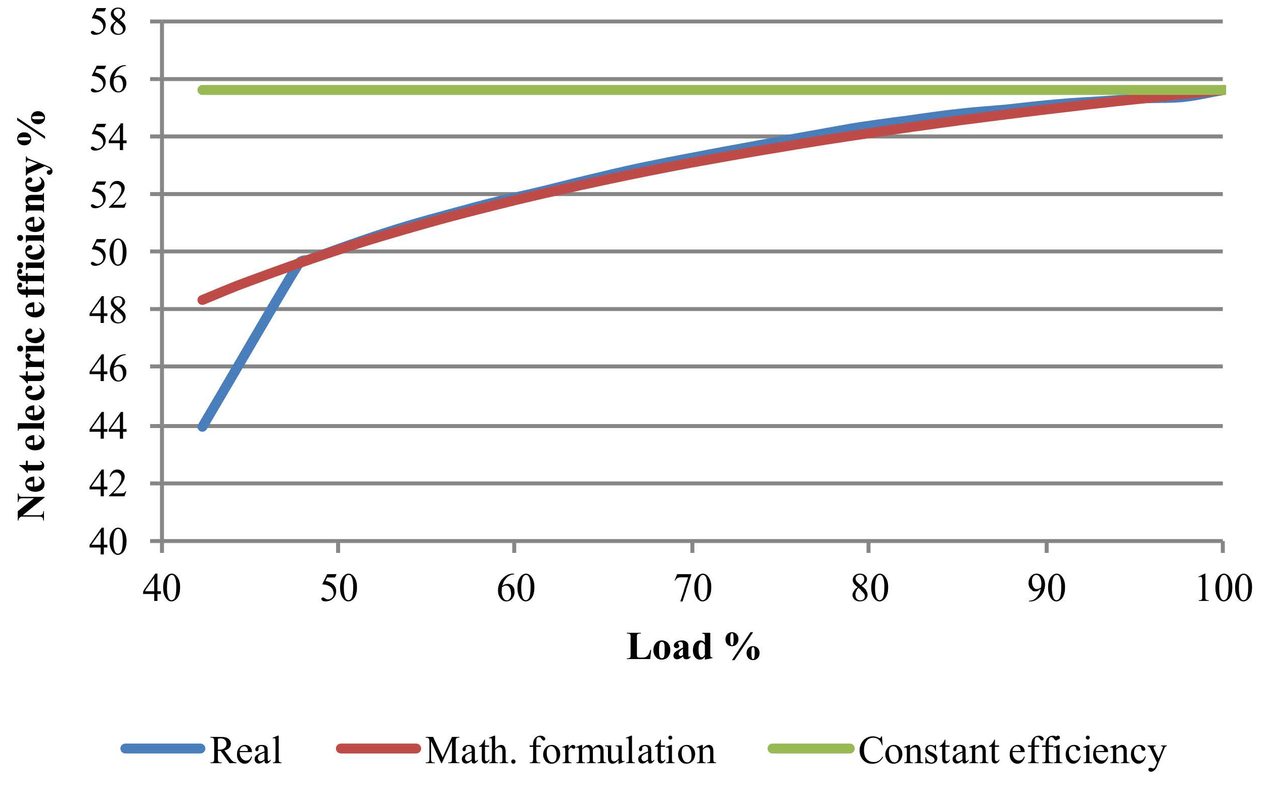
2.2. Cost of Fuel at Partial Load Operation

Usually, data in literature about the performance of power plants are aggregated, and a single number is provided as the efficiency of a technology—the full-load (i.e. nominal) efficiency. Therefore, energy system models assume the efficiency of individual power plants is constant and equal to its full-load value. The most advanced models consider for every technology two values of the efficiency—one at full load, one at partial load [9,32]. Assuming a constant efficiency, long-term energy system models compute the consumption of fuel as the product of the specific consumption by the generation in that time slice.
F C n o m = S C n o m · E
where E is the generation (PJ), S C n o m the nominal specific consumption of fuel (PJ/PJ), and F C n o m the total fuel consumption (PJ). According to (4), as S C n o m is constant, also the efficiency is constant and equal to the nominal value. Therefore, F C n o m decreases linearly with the load. However, in the real world the efficiency of thermal units, such as steam cycles, CCGTs, OCGTs, or nuclear power plants, decreases nonlinearly with the load [32,33,34]. If the formulation in Equation (4) is applied to scenarios where thermal units operate mostly at partial load, the consumption of fuel might be underestimated.
To overcome this risk, the efficiency needs to be a decreasing function of the load. However, directly representing the efficiency as a non-constant function of the load introduces non-linearities, which cannot be modelled in OSeMOSYS. Considering again Equation (4), if the efficiency varies with the generation E , so does S C , and the function F C becomes nonlinear. To overcome this problem, the functional relation of the efficiency on the load can be introduced in a different way. The fuel consumption F C at a load lower than the full load can be considered as the summation of the fuel consumption F C n o m in cases where the efficiency is constant and equal to its nominal value, plus a term of additional fuel consumption, proportional to the difference of the actual load to the full load:
F C = F C n o m + k · E f u l l   l o a d E
where the first term in the right-hand side is the fuel consumption at load E , in cases where the efficiency is equal to its nominal value. This is calculated as in Equation (4). The second term is an additional term of fuel consumption at load E , due to the decrease in the efficiency; k is a constant and it represents the additional fuel consumption per unit load (PJ/PJ). This is the only new parameter introduced in OSeMOSYS for this modification; E f u l l   l o a d is the energy the power plant would generate in the given time slice if it was operating constantly at full load. In this equation, F C is a linear function of E , as desired. The only term to be added into the original formulation of Equation (4) is, therefore, k · E f u l l   l o a d E ; k can be easily computed starting from the full-load and minimum-load efficiencies of a power plant, often available from literature or from the utilities. Since the efficiency is the inverse of the specific consumption, a linear variation of the latter will cause a nonlinear variation of the former, as shown in Equations (6) and (7):
1 η · E = 1 η n o m · E + k · E f u l l   l o a d E
η = η n o m · E E + η n o m · k · E f u l l   l o a d E
The hyperbolic decreasing trend of the efficiency in Equation (7) is nothing but a mathematical artefact, but it represents a much better approximation of reality, as shown in Figure 1. Here, the “real” curve refers to the operation of an existing combined cycle plant in Northern Italy, as presented in a previous study [35]; the simulated curve is computed through Equation (7), where k , η n o m , and E f u l l   l o a d are retrieved from the operation data of the same power plant.
The complete code formulation is presented in the supplementary material.

2.3. Refurbishment Option

In the past decade, energy utilities have been evaluating numerous refurbishment options or new operation practices to reduce the costs of the flexible operation of their thermal units and increase their capability to meet peak demand (suggested best practices have been reported in industrial literature [36,37]). Therefore, the power plant configuration and the corresponding cycling capability are variables of the energy system configuration—they can be optimised together with the supply mix as functions of costs and demands, in order to assess least-cost options to increase reliability of supply in scenarios with significantly increasing penetration of intermittent renewables.
The present modification allows the configuration of specific technologies (chosen by the user through a “tag”) to vary discretely and makes the performance of the technology a function of these discrete variables. This is done assuming that two configurations, or versions, of a technology are allowed—an old and a new one. The old version represents the original power plant, while the new version represents the refurbished one. The user defines a priori the characteristics of the two versions, by assigning values to all the parameters of each one. The model is allowed at every moment to decommission part of the installed capacity of the old version and install at most a corresponding capacity of the new version. The cost for replacing old with new capacity corresponds to the sole cost of refurbishment. Seven new equations and two modified equations are introduced in OSeMOSYS to allow for these dynamics. For simplicity, in this paragraph only the rationale of the modification is described. The whole set of the constraints for this code modification is presented (both in algebraic form and in code formulation) in the additional material:
  • The first set of constraints defines the withdrawn capacity of the old version of the technology as the sum of the one fictitiously retired to be replaced by the refurbished capacity, and the one actually decommissioned;
  • The second set of constraints defines the refurbished capacity as a capacity of the new technology equalling that of the old technology that is fictitiously retired;
  • Finally, the third set of constraints only consists of a number of equations of the original code, updated to account for the refurbished capacity and the cost of the refurbishment.

2.4. Test Case Study

The enhanced OSeMOSYS code is tested by application to a simple and aggregated representation of the Italian electricity system. The application is deliberately kept simple as its purpose is to test the relevance of the model improvements rather than to derive recommendations regarding the technology mix. Sensitivity analyses on a number of parameters are introduced only at a later stage (see Section 3) to illustrate what messages may emerge in situations closer to reality.
The structure of the system under study is shown in Figure 2. This depicts the Reference Energy System (RES) of the case study, i.e., a schematic and aggregated representation of the electricity supply chain commonly used for modelling purposes.
On the right-hand side, the RES shows that one electricity demand is considered, cumulating demands from all the sectors of the economy. Additionally, reserve capacity demands are taken into account to study their impact on balancing requirements. Moving to the left, three types of power plants provide electricity: solar photovoltaic panels (PV), representative of variable renewables, Coal-fired power plants (Coal PP), and Combined Cycle Natural Gas-fired power plants (NGCC). At the start of the modelling period, Coal PP and NGCC exist to meet the electricity demand. In the following years, these are slowly decommissioned and need to be replaced by new capacity of any power plant. Combined power plants of a new generation (NGCCupg) may be built or derived from upgrade of old ones. On the left-hand side, the non-renewable primary resources are shown—coal and natural gas. For the purpose of the case study, no information on whether the sources are mined domestically or imported is required, therefore no differentiation is made.
The structural and scenario-independent model parameters of the case study are listed in Table 1.
The choice of 2014 as the base year is due to the large availability of data to calibrate the model. The partition into 16 time slices is motivated by the need to capture the most important parts (including peaks) of the electricity load curve and the availability of solar power. It can be easily increased up to a few hours resolution if needed, but this is unnecessary for the illustration purposes of this paper. The trend of electricity demand from 2014 to 2040 is built upon Terna statistical data [7]: the electricity demand in Italy in 2014 was 291 TWh and a growth of 1% is applied thereafter. This trend follows the one assumed by Terna in its Piano di Sviluppo 2015 for the Development Scenario [36]. The ratio of annual demand occurring in each time slice is derived using load curves for the electricity demand in Italy, as from a previous study [7]. The demand for reserve capacity upwards and downwards in 2014 is assumed as the sum of secondary and tertiary reserve capacity demand reported by Terna [7]. Primary reserve (faster and shorter-term) is not considered here out of simplicity, but it could seamlessly be introduced as well. The reserve is assumed to increase at the same rate as the electricity demand, i.e., 1% annually. The CO2 price is assumed to be constant and close to the historical minimum values reached in 2013 (and again at moments in 2016 and 2017), as reported in Appendix 2 of a previous study [38]. The minimum value was chosen as a base assumption, upon which sensitivities may be built. Sensitivity analyses around this value are shown in Section 3.
Table 2 lists the main techno-economic assumptions related to power supply options.
The values for cost and efficiency of the Coal PP, NGCC, and PV technologies (including fuel costs) are taken from a previous study [39] (see values for: supercritical coal power plants on page 30, Table 2.2, right column; 800 MW combined cycles on page 39, Table 2.3, right column; and centralised 2 MW ground PV fields on page 62, Table 2.8, bottom row). All costs of NGCCupg are assumed to be equal to those of NGCC, except for the capital costs. These are assumed to be higher than those for NGCC by an amount required to install equipment to improve the ramping capability of the power plants. Such figures are purely indicative and hardly referenced, since exact values cannot be disclosed by power plant operators. However, they are in the order of magnitude that a set of real retrofits may require (as those discussed in a previous study [35]). The assumption is considered sufficient for the purpose of this study. Costs are assumed to remain constant throughout the time domain of the study. The CO2 emission factors are the average within the ranges provided by the ETSAP database [40]. Table 3 represents the additional techno-economic assumptions needed to compute the newly introduced parameters.
The minimum stable operation and the efficiency at minimum load of NGCC and NGCCupg are derived in a previous study [35] by the authors from a detailed study of the operation of a real power plant in Italy. The same values for Coal PP are assumed from literature. For each power plant type, the two values are used to compute factor k , according to Equation (7). This is used as an input parameter for the code additions in OSeMOSYS. The maximum ramping rate is assumed from a previous study [41]. Since OSeMOSYS requires the maximum ramping rate to be input as % of the full load, assumptions are made regarding (a) the average full capacity of a power plant for each of the fossil fuel fired technologies and (b) the time by which the reserve must be provided. The former is assumed as 400 MW for coal and 390 MW for natural gas power plants [41]; the latter is assumed as 15 min, which is the time required for the “prompt” tertiary reserve provision in Italy [42] and the same time range used in [9]. The cost of ramps per unit of capacity of Coal PP, NGCC, and NGCCupg is derived from a previous study [31], as the median cost of a warm start up for supercritical coal power plants, gas combined cycle units, and Best Available Technology combined cycle units, respectively. Finally, the cost of retrofit is assumed to be in the order of magnitude of the one of a set of retrofits to improve the ramping capability of combined cycles, as from a previous study [35]. It also corresponds, out of simplification, to the difference in capital cost between existing and newly built combined cycles.
With this model structure, two scenarios are investigated:
  • RETarget: A renewable generation target is imposed. It equals 37.5% in 2014, as reported by IEA [43], and it is assumed to grow at the constant rate of 1% and reach 63.5% in 2040, in line with the Italian Government’s 2013 National Energy Strategy [44].
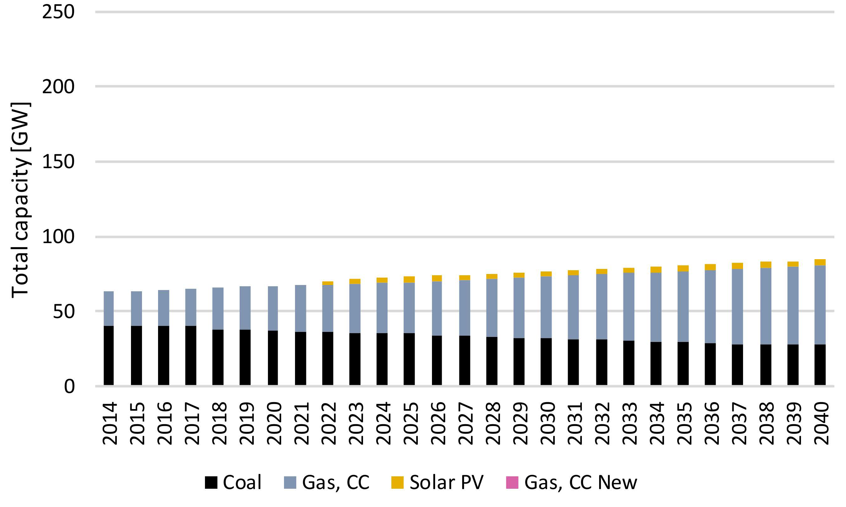
  • REF: a reference scenario where no target is imposed.

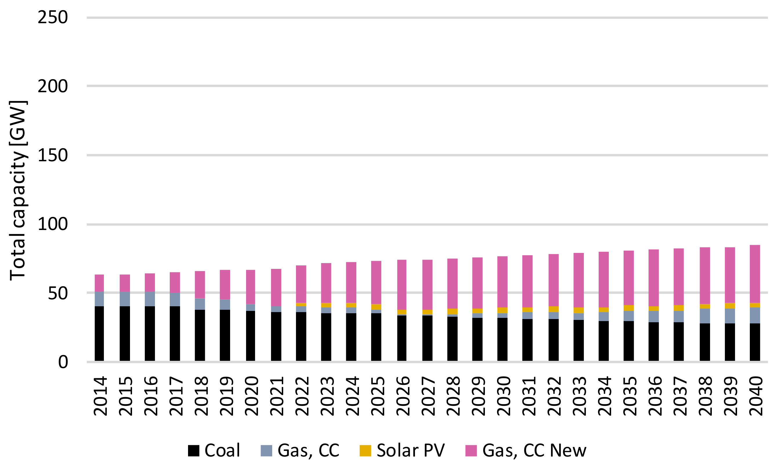
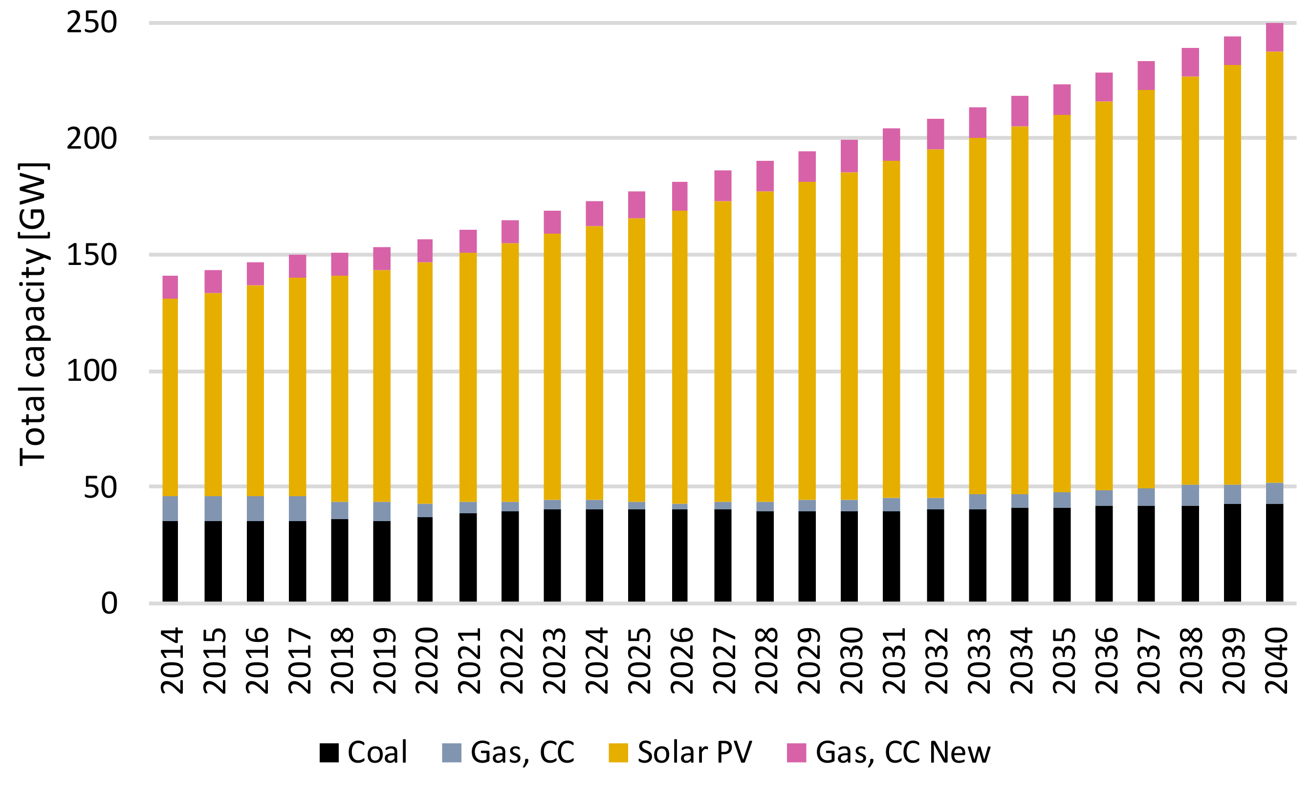
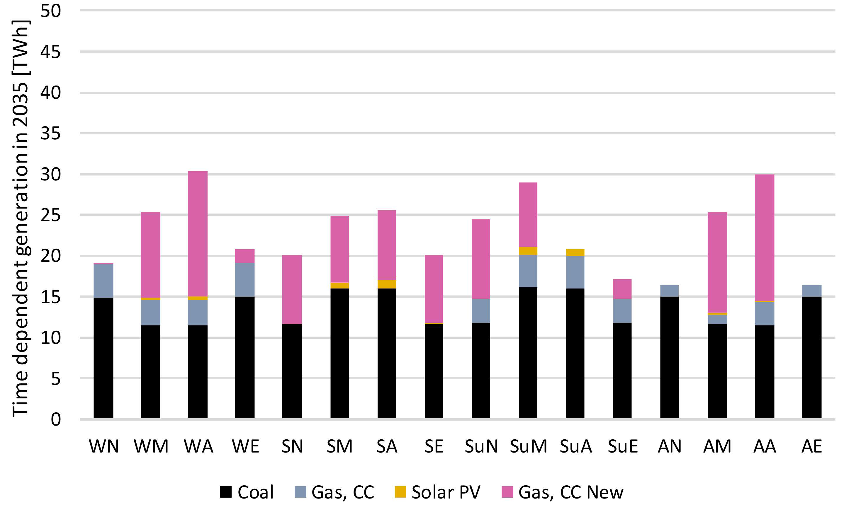
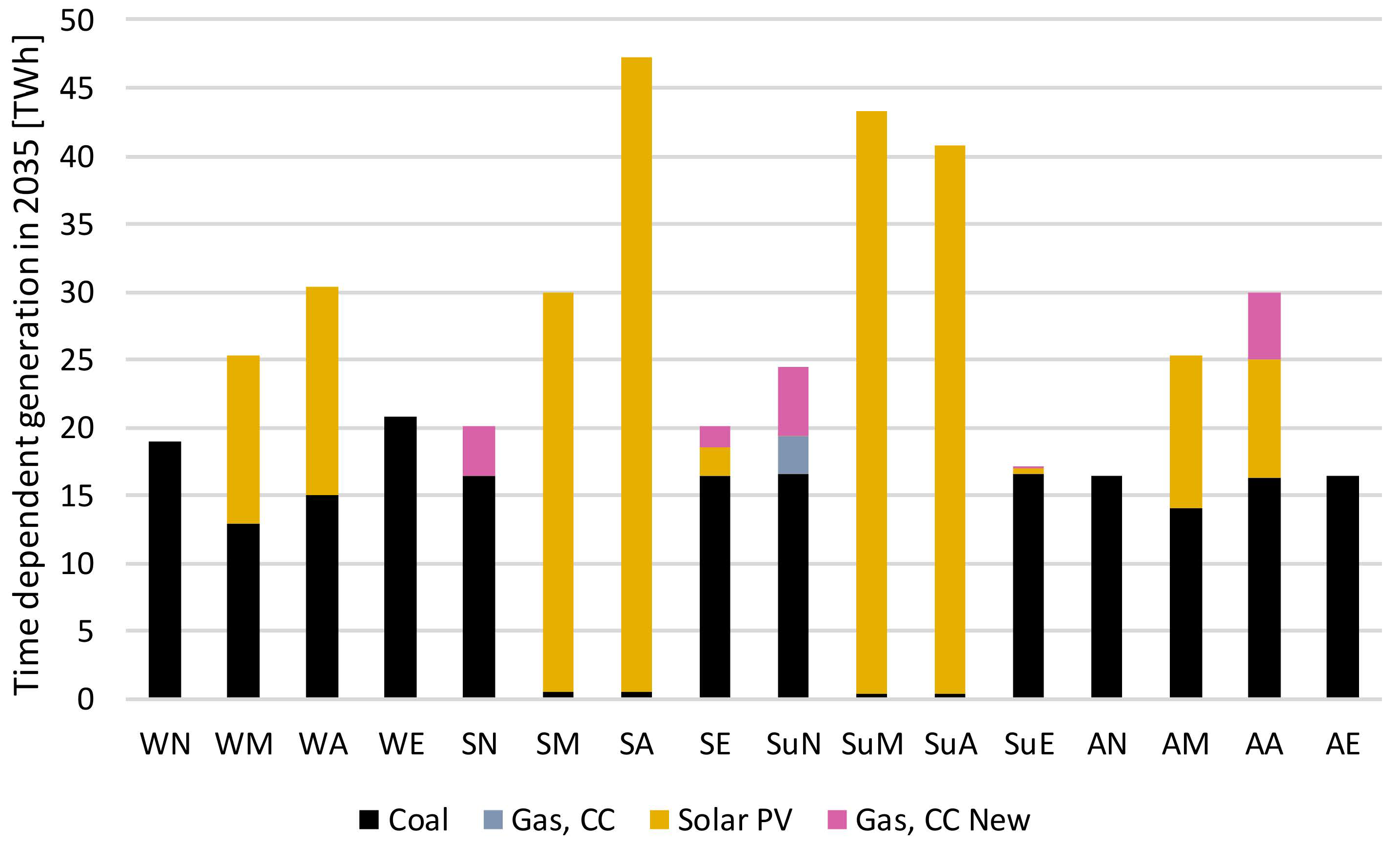
3. Results and Discussion

The OSeMOSYS code including the described enhancements was applied to the test case study presented in Section 2.4 and compared with the original code. Key output metrics and relative insights for the REF and RETarget scenarios are shown in the following.

3.1. Without Code Modifications

Firstly, results for applying the original, yet enhanced, formulation of OSeMOSYS which considers operating reserves are presented. Results based on the improvements introduced in this paper are presented thereafter. Results as in Figure 3 and Figure 4 are obtained for the REF and the RETarget scenarios regarding the investments in generation capacity (the same scale is used in the two graphs, to better show investment trade-offs between renewable and non-renewable options).
In the REF scenario, the future least cost production mix relies heavily on fossil fuels, with gradual replacement of coal power plants with the more efficient and less CO2-intensive natural gas combined cycles.
Without the improvements suggested in this paper, new more flexible combined cycles are not deemed competitive; only old generation combined cycles are employed to meet current and future energy needs. Without the improvements, more and less flexible combined cycles could only be distinguished in OSeMOSYS through difference in the minimum stable generation rate or the capability to contribute to reserve. However, in reality less and more flexible options differ not only by these characteristics. The efficiencies at part-load and start-up costs may also matter, as the case reported here (based on real numbers) shows. With the current cost assumptions, large scale centralised solar PV generation is not competitive.
In the RETarget scenario, where a minimum renewable generation target is added, significant investments in solar PV are made (Figure 4). The total capacity is considerably higher than the in the REF scenario because, on top of the existing capacity of thermal power plants, solar PV is needed to meet the renewable generation targets. The capacity is higher already in past years (starting 2014) because the target for renewable generation is imposed, out of simplicity, from the first year of the modelling domain. As solar PV is not cost competitive compared to coal and gas, in the least-cost solution prospected by OSeMOSYS it generates no more than the minimum required by the target. Within the thermal generation, the same competition between coal power plants and old generation natural gas combined cycles happens, as in the REF scenario.
By analysing the generation profile within one year (Figure 5 and Figure 6) and the provision of reserve capacity (Figure 7 and Figure 8) in the two scenarios, important indications can be drawn. Coal power plants are used for base load, intermediate, and peak load generation, while combined cycles provide only intermediate and peak load generation (to a greater extent in the REF scenario, and to a lesser extent in the RETarget scenario).

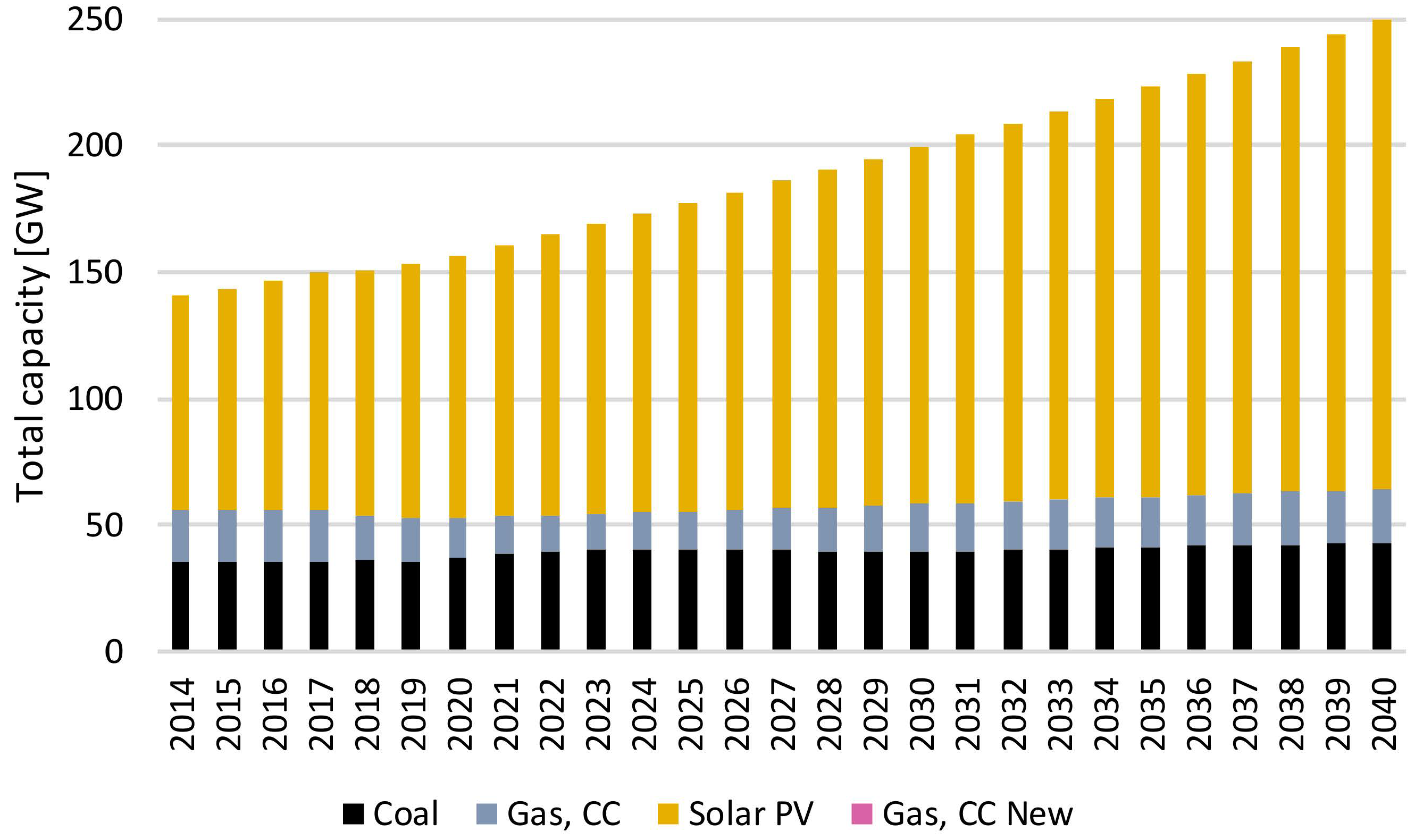
3.2. With Code Modifications

When the enhanced formulation is applied to the two scenarios, the results change significantly, as shown in Figure 9 and Figure 10.
In the REF scenario, where thermal generation is dominant, competition between old and new generation combined cycles emerges for providing intermediate and peak load generation. This is due to the assumption of new generation combined cycles having lower ramping costs and a higher minimum load efficiency. The new generation combined cycles are both a result of construction of new power plants and retrofit of old ones. Specifically, in the REF scenario, around 10 GW of old generation combined cycles are replaced by new ones already in the first year, as a result of retrofit operations (the latter may be verified also in the detailed results annexed as supplementary materials). With the current assumptions on costs of retrofit (constant across the time period), the least cost solution is naturally to operate all retrofits as early as possible in the analysed period. Notice that changes in other techno-economic characteristics may be easily introduced by the user, such as lower variable Operation and Maintenance (O&M) costs, lower CO2 emission factors, or higher full load efficiency. What is shown here is just one specific case corresponding to a given set of improvements in the old generation technology.
In accordance with the results shown above, new generation combined cycles gain a share in the intermediate and peak load generation and in the supply of reserve capacity, replacing old combined cycles in many instances (Figure 11, Figure 12, Figure 13 and Figure 14). In Figure 13 it is interesting to note that old NGCCs become less attractive for providing reserve capacity. If they were to provide it, they should operate longer times at partial load. However, their efficiency decreases more than the one of new combined cycles at partial load. Therefore, the latter become more attractive, or coal power plants in time slices where new combined cycles are not dispatched (see Figure 11).
For the RET scenario, Figure 12 shows that old combined cycles are rarely ever dispatched, and thus not available as reserve, therefore new combined cycles completely take over the role the old ones previously performed (Figure 14).
As mentioned above, the cost of retrofits was assumed to be constant throughout the time domain of the study. Consequently, the cost optimal solution was to carry out all necessary retrofits to old combined cycles in the first year. Assuming a learning curve for the costs of retrofits along the time domain of the study, from a higher value than previously assumed to a lower value, will result in different indications on when it could be cost effective to perform retrofit operations. An example is shown in Figure 15. By assuming an initial cost of retrofit of 5 M€/GW, decreasing by 5% every year until 2020, around 3.5 GW of old generation combined cycles are refurbished in 2018 and 2.5 GW in 2020.
The results of the test case study are sensitive to cost assumptions, but the indications on the competitiveness between balancing options drawn with the code modifications are not.
In this simplified case, all costs were assumed to remain constant across the time domain of the study. While such assumption may be reasonable for mature technologies, such as coal power plants and natural gas combined cycles, it is less so for instance for fuel prices, solar PV capital costs, and carbon prices. The implications of changing prices are analysed in the following.
By assuming a linear increase of the gas prices by 1% every year, the results shown in Figure 16 and Figure 17 are obtained for the REF scenario, respectively, with original and modified code. Due to increasing gas prices, the shares of the technologies in electricity generation change in both cases and solar PV becomes gradually more competitive with gas generation. On top of this change, the addition of the new functionalities to OSeMOSYS introduces the competition between the less and more flexible versions of the combined cycle technology (Figure 17). This additional insight obtained in the previous cases is confirmed.
The same dynamics are observed if the capital costs of solar PV and the carbon prices are changed. A sensitivity analysis over the REF scenario is made, where (1) solar PV costs decrease linearly from 1200 €/kW in 2014 to 800 €/kW in 2040 and (2) the carbon tax increases linearly to reach 80 €/ton in 2030 and keeps increasing at the same pace thereafter. The resulting installed capacity (GW) without and with code modifications can be observed in Figure 18 and Figure 19, respectively. The new assumptions result in solar PV becoming strongly competitive after 2030 and the favourite option for investments to meet the increasing electricity demand. The large increase in the total capacity is due to the low average capacity factors assumed for solar PV. The generation of solar PV increases, particularly at the expense of coal generation. In the last years of the modelling period, natural gas power plants are used more for generation, while coal power plants are used more for reserve capacity supply. The same outlook for solar PV is observed without and with the code modifications. The difference between the two cases lies again in the competitiveness of old generation and new generation combined cycles and confirms the previous findings.

4. Conclusions

This paper aims to improve the capability of energy modelling tools of providing investment outlooks for long-term planning, in cases where highly flexible generation and high penetration of intermittent renewables are expected. It uses and generates transparent and open-to-all tools, accessible high-quality data, and reproducible benchmarks in order to deepen the impact and enlarge the outreach of modelling results at several levels of decision-making processes.
Specifically, the authors introduce functionalities into an open source long-range energy system modelling framework to account for the costs of flexible generation to back up intermittent renewables. The added functionalities relate to cost of ramps, fuel cost for partial load operation, and refurbishment options. The code modifications bring the following contributions to established practice:
  • They are highly accessible to the modelling community, including non-expert modellers: they are open source licensed, documented at several levels (plain description, algebraic formulation, and code) and explained step by step in the supplementary materials. This contributes to the establishment of standards for the development of an open source modelling tool and the creation of benchmarks. Building on practices initiated in previous studies, it provides a proof of concept for open source incremental changes to OSeMOSYS, including code and model documentation, licenses, and metadata, and a retrievable, reproducible, reusable, interoperable, and auditable case study.
  • They are simple to use: they consist of a limited number of additional equations and input parameters, thus requiring minimum additional effort on the user’s side regarding their integration into a model.
  • They are linear: yet they allow the introduction of non-linear behaviour, such as when modelling the cost of fuel at partial load operation (see Figure 1 and Equation (6)). This enables a realistic representation with limited computational requirements.
The enhanced modelling framework proves useful for the purpose of studying long-term investment options in scenarios with high renewable penetration. Its application to a test case study provides two main insights: costs of ramping and decreased partial load efficiency may influence the competitiveness of generation technologies in the provision of reserve capacity; and refurbishments of existing power generation units may represent attractive options to provide flexibility to back up variable renewables. Both effects are seen also in the long-term and may impact infrastructure investment decisions to meet decarbonisation targets.
The enhanced modelling framework can be of use for planning energy infrastructure investments in scenarios where high renewable penetration is targeted and it is expected to be backed up by non-renewable generation, amongst other options. One such case occurs for instance in Tunisia, where the authors are contributing to modelling efforts to support energy supply plans [45]. Here, targets of renewable penetration combine with limited electricity trade capacity with neighbouring countries, limited hydro resources, need for security of supply, and abundance of fossil resources. Another case is Ireland, where the authors initiated similar modelling work to support the introduction of high shares of renewable electricity [21]. The enhancements to the modelling framework may also be of use separately. For instance, the refurbishment option may be employed for power plant life extensions, which in some instances could have impacts on the transition to a new energy supply mix [46]. On the contrary, the code enhancements presented in this paper may be of more limited use in cases where hydro power plants with dams and interconnections between countries provide most of the necessary flexibility and security of supply.
Future work will focus on the introduction of additional functionalities to compute the reserve capacity demand as a function of the penetration of intermittent renewables and their variability, based on work initiated by Maggi in a previous study [47]. The enhanced modelling framework will also be applied to real case studies, featuring more complex energy mix and actual cost trends, to extract policy insights. Application is under development for the Tunisian model developed in a previous study [45]. The engagement with local institutions for future work was made possible by the relevance, accessibility, and documentation of the enhanced modelling framework.

supplementary materials

Input data sources and calculations (.xlsx); code modifications (.docx); code files (.txt); test case study data files (.txt.); test case study metadata (.json); results files (.xlsx and .txt.). The supplementary materials are available online at https://www.mdpi.com/1996-1073/12/12/2366/s1.

Author Contributions

All authors contributed significantly to the work. They contributed equally to the conceptualization. The development of the methodology, software update, and validation was carried out by Francesco Gardumi and Manuel Welsch. The original draft preparation was carried out by F.G., while the review was carried out by M.W., E.C., and M.H.

Funding

This research received no external funding.

Conflicts of Interest

The authors declare no conflict of interest.

Acronyms and Nomenclature
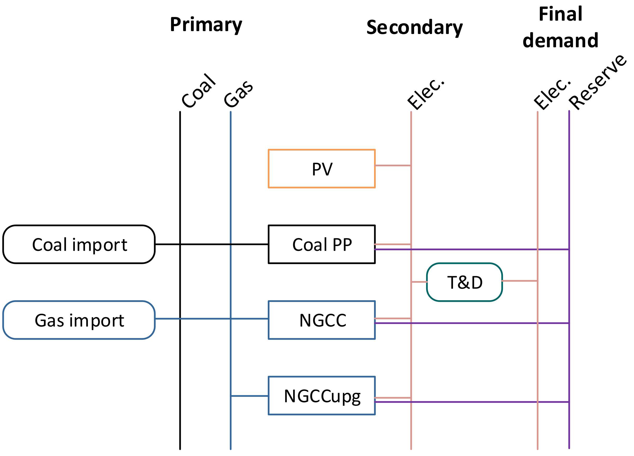
NGCCNatural Gas Combined Cycle
Coal PPCoal Power Plants
RESReference Energy System
WNWinter night
WMWinter morning
WAWinter afternoon
WEWinter evening
SNSpring night
SMSpring morning
SASpring afternoon
SESpring evening
SuNSummer night
SuMSummer morning
SuASummer afternoon
SuESummer evening
ANAutumn night
AMAutumn morning
AAAutumn afternoon
AEAutumn evening
REFReference scenario
RETargetRenewable Energy Target scenario

References

  1. European Commission. Communication from the Commission to the European Parliament, the Council, the European Economic and Social Committee, the Committee of the Regions and the European Investment Bank on ’A Framework Strategy for a Resilient Energy Union with a Forward-Looking Climate Change Policy; European Commission: Brussels, Belgium, 2015. [Google Scholar]
  2. International Energy Agency (IEA). World Energy Outlook 2017; International Energy Agency (IEA): Paris, France, 2017. [Google Scholar]
  3. International Renewable Energy Agency. Renewable Power Generation Costs in 2017; International Renewable Energy Agency: Abu Dhabi, UAE, 2018. [Google Scholar]
  4. OECD/IEA; IRENA. Perspectives for the Energy Transition: Investment Needs for a Low-Carbon Energy System; IRENA: Abu Dhabi, UAE, 2017. [Google Scholar]
  5. Shivakumar, A.; Taliotis, C.; Deane, P.; Gottschling, J.; Pattupara, R.; Kannan, R.; Jakšić, D.; Stupin, K.; Hemert, R.V.; Normark, B.; et al. Need for Flexibility and Potential Solutions. In Europe’s Energy Transition—Insights for Policy Making; Elsevier: Amsterdam, The Netherlands, 2017; pp. 149–172. [Google Scholar]
  6. Falchetta, M. Fonti Rinnovabili e rete Elettrica in Italia. Considerazioni di Base e Scenari di Evoluzione delle Fonti Rinnovabili Elettriche in Italia; ENEA: Rome, Italy, 2014. [Google Scholar]
  7. Terna. Dati Statistici 2015. Available online: https://www.terna.it/it-it/sistemaelettrico/statisticheeprevisioni/datistatistici.aspx (accessed on 14 May 2019).
  8. European Commission. Consultation Paper on Generation Adequacy, Capacity Mechanisms and the Internal Market in Electricity; European Commission: Brussels, Belgium, 2012. [Google Scholar]
  9. Welsch, M.; Howells, M.; Hesamzadeh, M.; OGallachoir, B.; Deane, P.; Strachan, N.; Bazilian, M.; Kammen, D.M.; Jones, L.; Strbac, G.; et al. Supporting security and adequacy in future energy systems: The need to enhance long-term energy system models to better treat issues related to variability. Int. J. Energy Res. 2015, 39, 377–396. [Google Scholar] [CrossRef]
  10. PLEXOS® Simulation Software. Energy Ex n.d. Available online: https://energyexemplar.com/products/plexos-simulation-software/ (accessed on 11 October 2018).
  11. Prina, M.G.; Cozzini, M.; Garegnani, G.; Manzolini, G.; Moser, D.; Filippi Oberegger, U.; Pernettia, R.; Vaccaroa, R.; Sparber, W. Multi-objective optimization algorithm coupled to EnergyPLAN software: The EPLANopt model. Energy 2018, 149, 213–221. [Google Scholar] [CrossRef]
  12. Prina, M.G.; Fanali, L.; Manzolini, G.; Moser, D.; Sparber, W. Incorporating combined cycle gas turbine flexibility constraints and additional costs into the EPLANopt model: The Italian case study. Energy 2018, 160, 33–43. [Google Scholar] [CrossRef]
  13. Hörsch, J.; Hofmann, F.; Schlachtberger, D.; Brown, T. PyPSA-Eur: An open optimisation model of the European transmission system. Energy Strategy Rev. 2018, 22, 207–215. [Google Scholar] [CrossRef] [Green Version]
  14. Brinkerink, M.; Shivakumar, A. System dynamics within typical days of a high variable 2030 European power system. Energy Strategy Rev. 2018, 22, 94–105. [Google Scholar] [CrossRef]
  15. Schrattenholzer, L. The Energy Supply Model MESSAGE; IIASA: Laxenburg, Austria, 1981. [Google Scholar]
  16. Loulou, R.; Remme, U.; Kanudia, A.; Lehtila, A.; Goldstein, G. Documentation for the TIMES Model Part I; IEA-ETSAP: Paris, France, 2005. [Google Scholar]
  17. The Balmorel Open Source Project—Home n.d. Available online: http://www.balmorel.com/ (accessed on 11 October 2018).
  18. Howells, M.; Rogner, H.; Strachan, N.; Heaps, C.; Huntington, H.; Kypreos, S.; Hughes, A.; Silveira, S.; DeCarolis, J.; Bazillian, M.; et al. OSeMOSYS: The Open Source Energy Modeling System: An introduction to its ethos, structure and development. Energy Policy 2011, 39, 5850–5870. [Google Scholar] [CrossRef]
  19. Connolly, D.; Lund, H.; Mathiesen, B.; Leahy, M. A review of computer tools for analysing the integration of renewable energy into various energy systems. Appl. Energy 2010, 87, 1059–1082. [Google Scholar] [CrossRef]
  20. Ludig, S.; Haller, M.; Schmid, E.; Bauer, N. Fluctuating renewables in a long-term climate change mitigation strategy. Energy 2011, 36, 6674–6685. [Google Scholar] [CrossRef]
  21. Welsch, M.; Deane, P.; Howells, M.; OGallachoir, B.; Rogan, F.; Bazilian, M.; Rogner, H. Incorporating flexibility requirements into long-term energy system models—A case study on high levels of renewable electricity penetration in Ireland. Appl. Energy 2014, 135, 600–615. [Google Scholar] [CrossRef]
  22. Gardumi, F. Personal GitHub. Gardumi OSeMOSYS Repos n.d. Available online: https://github.com/FraGard/OSeMOSYS/tree/master/addons (accessed on 14 May 2019).
  23. Communication from the Commission to the European Parliament, the Council, the European Economic and Social Committee and the Committee of the Regions: European Cloud Initative—Building a Competitive Data and Knowledge Economy in Europe; European Commission: Brussels, Belgium, 2016.
  24. Taliotis, C.; Rogner, H.; Ressl, S.; Howells, M.; Gardumi, F. Natural gas in Cyprus: The need for consolidated planning. Energy Policy 2017, 107, 197–209. [Google Scholar] [CrossRef]
  25. Taliotis, C.; Shivakumar, A.; Ramos, E.P.; Howells, M.; Mentis, D.; Sridharan, V.; Broad, O.; Mofor, L. An indicative analysis of investment opportunities in the African electricity supply sector—Using TEMBA (The Electricity Model Base for Africa). Energy Sustain. Dev. 2016, 31, 50–66. [Google Scholar] [CrossRef]
  26. Pinto de Moura, G.N.; Loureiro Legey, L.F.; Balderrama, G.P.; Howells, M. South America power integration, Bolivian electricity export potential and bargaining power: An OSeMOSYS SAMBA approach. Energy Strategy Rev. 2017, 17, 27–36. [Google Scholar] [CrossRef]
  27. Henke, H. The Open Source Energy Model Base for the European Union (OSEMBE). 2017. Available online: https://aaltodoc.aalto.fi/bitstream/handle/123456789/27115/master_Henke_Hauke_2017.pdf?sequence=1&isAllowed=y (accessed on 14 June 2019).
  28. Huntington, H.; Weyant, J.; Sweeney, J. Modeling for insights, not numbers: The experiences of the energy modeling forum. Omega 1982, 10, 449–462. [Google Scholar] [CrossRef]
  29. OSeMOSYS Community of Practice. OSeMOSYS.org n.d. Available online: http://www.osemosys.org/ (accessed on 14 May 2019).
  30. Gardumi, F.; Shivakumar, A.; Morrison, R.; Taliotis, C.; Broad, O.; Beltramo, A.; Sridharan, V.; Howells, M.; Hörsch, J.; Niet, T.; et al. From the development of an open-source energy modelling tool to its application and the creation of communities of practice: The example of OSeMOSYS. Energy Strategy Rev. 2018, 20, 209–228. [Google Scholar] [CrossRef]
  31. Kumar, N.; Besuner, P.; Lefton, S.; Agan, D.; Hilleman, D. Power Plant Cycling Costs; National Renewable Energy Laboratory: Sunnyvale, CA, USA, 2012.
  32. IEA. Power Generation from Coal Measuring and Reporting Efficiency Performance and CO2 Emissions; IEA: Paris, France, 2010. [Google Scholar]
  33. Lucquiaud, M.; Fernandez, E.; Chalmers, H.; Mac Dowell, N.; Gibbins, J. Enhanced operating flexibility and optimised off-design operation of coal plants with post-combustion capture. Energy Procedia 2014, 63, 7494–7507. [Google Scholar] [CrossRef]
  34. Kim, T. Comparative analysis on the part load performance of combined cycle plants considering design performance and power control strategy. Energy 2004, 29, 71–85. [Google Scholar] [CrossRef]
  35. Gardumi, F. A Multi-Dimensional Approach to the Modelling of Power Plant Flexibility. Ph.D. Thesis, Politecnico di Milano, Milan, Italy, 2016. [Google Scholar]
  36. Terna S.p.A. Piano di Sviluppo 2015 n.d. Available online: https://www.arera.it/allegati/operatori/pds/PdS%202015_Gennaio%202015.pdf (accessed on 14 May 2019).
  37. Venkataraman, S.; Jordan, G.; O’Connor, M. Cost-Benefit Analysis of Flexibility Retrofits for Coal and Gas-Fueled Power Plants; NREL: Golden, CO, USA, 2013.
  38. European Commission. Report from the Commission to the European Parliament and the Council: Report on the Functioning of the European Carbon Market; European Commission: Brussels, Belgium, 2018. [Google Scholar]
  39. Energetico, R.S. Energia Elettrica, Anatomia dei Costi: Aggiornamento Dati al 2015; Editrice Alkes: Milano, Italy, 2015. [Google Scholar]
  40. IEA-ETSAP. Energy Supply Technologies Data 2015. Available online: http://109.73.233.125/~ieaetsap/index.php/energy-technology-data/energy-supply-technologies-data (accessed on 14 May 2019).
  41. Meibom, P.; Barth, R.; Brand, H.; Hasche, B.; Swider, D.; Ravn, H. Final Report for All Island Grid Study Work-stream 2 (b): Wind Variability Management Studies; Riso National Laboratory: Roskilde, Denmark, 2007. [Google Scholar]
  42. Di Rete, C. Capitolo 4: Regole per il Dispacciamento; Terna S.p.A.: Rome, Italy, 2015. [Google Scholar]
  43. International Energy Agency (IEA). Country Statistics. Stat Glob Energy Data Your Fingertips 2017. Available online: https://www.iea.org/statistics/statisticssearch/report/?country=Mozambique&product=balances (accessed on 14 May 2019).
  44. Ministero dello Sviluppo Economico. Strategia Energetica Nazionale: Per Un’energia Più Competitiva E Sostenibile; Italian Government: Rome, Italy, 2013.
  45. Dhakouani, A.; Gardumi, F.; Znouda, E.; Bouden, C.; Howells, M. Long-term optimisation model of the Tunisian power system. Energy 2017, 141, 550–562. [Google Scholar] [CrossRef]
  46. International Energy Agency. Nuclear Power in a Clean Energy System; International Energy Agency: Paris, France, 2019. [Google Scholar]
  47. Maggi, C. Accounting for the Long Term Impact of High Renewable Shares through Energy System Models: A Novel Formulation and Case Study. Master’s Thesis, Politecnico di Milano, Milano, Italy, 2016. [Google Scholar]
Figure 1. Comparison between the curves of the efficiency as from the proposed mathematical formulation, models featuring constant efficiency, and a real CCGT.
Energies 12 02366 g001
Figure 2. Reference Energy System (RES) of the case study.
Energies 12 02366 g002
Figure 3. Total capacity (GW) in the REF scenario—without code modifications.
Energies 12 02366 g003
Figure 4. Total capacity (GW) in the RETarget scenario—without code modifications.
Energies 12 02366 g004
Figure 5. Generation (TWh) per time slice in 2035 in REF scenario—without code modifications.
Energies 12 02366 g005
Figure 6. Generation (TWh) by time slice in 2035 in the RETarget scenario—without code modifications.
Energies 12 02366 g006
Figure 7. Reserve capacity supply (GW) per time slice in 2035 in REF scenario—without code modifications.
Energies 12 02366 g007
Figure 8. Reserve capacity supply (GW) in 2035 in the RETarget scenario—without code modifications.
Energies 12 02366 g008
Figure 9. Total capacity (GW) in the REF scenario—with code modifications.
Energies 12 02366 g009
Figure 10. Total capacity (GW) in the RETarget scenario—with code modifications.
Energies 12 02366 g010
Figure 11. Generation (TWh) per time slice in 2035 in the REF scenario—with code modifications.
Energies 12 02366 g011
Figure 12. Generation (TWh) per time slice in 2035 in the RETarget scenario—with code modifications.
Energies 12 02366 g012
Figure 13. Reserve capacity supply (GW) per time slice in 2035 in the REF scenario—with code modifications.
Energies 12 02366 g013
Figure 14. Reserve capacity supply (GW) per time slice in 2035 in the RETarget scenario—with code modifications.
Energies 12 02366 g014
Figure 15. Total capacity (GW) in the REF scenario, in cases of decreasing cost of retrofit—with code modifications.
Energies 12 02366 g015
Figure 16. Total capacity (GW) in the REF scenario, in cases of higher gas prices—without code modifications.
Energies 12 02366 g016
Figure 17. Total capacity (GW) in the REF scenario, in cases of higher gas prices—with code modifications.
Energies 12 02366 g017
Figure 18. Total capacity (GW) in the REF scenario, in cases of decreasing solar PV capital costs and increasing CO2 tax—without code modifications.
Energies 12 02366 g018
Figure 19. Total capacity (GW) in the REF scenario, in cases of decreasing solar PV capital costs and increasing CO2 tax—with code modifications.
Energies 12 02366 g019
Table 1. Structural and scenario-independent inputs for the case study.
Time Domain2014–2040
Time split16 time slices: night, morning, afternoon, evening-4 seasons 1
Electricity demand291 TWh in 2014, then increasing at constant rate of 1%
Upward reserve capacity demand4.61 GW in 2014, then increasing at constant rate of 1%
Downward reserve capacity demand2.17 GW in 2014, then increasing at constant rate of 1%
Taxations4 €/ton CO2, constant
Price of coal2.63 €/GJ, constant
Price of gas8.08 €/GJ, constant
Discount rate5%
1 The naming of the time slices, useful for reading the following figures, is described in the nomenclature.
Table 2. Main techno-economic assumptions of the case study.
ParameterPVCoal PPNGCCNGCCupg
Capital Costs [M€/GW]12001750650653
Variable Costs [M€/PJ]6.4200.6940.8750.875
Fixed Costs [M€/GW]203510.510.5
Fuel Cost [M€/PJ]02.68.18.1
Efficiency at full load [%]10041.15656
CO2 emission factor [Mton/PJ]00.2190.1030.103
Operational life (years)30353030
Table 3. Additional techno-economic assumptions for the case study.
ParameterPVCoal PPNGCCNGCCupg
Minimum Stable Operation [% of full load]0454242
Efficiency at min stable operation [%]0374448
Max ramping rate [MW/min]081111
Cost of starts [M€/GW]00.0500.0430.034
Cost of retrofit [M€/GW]0003

