Adaptive Forgetting Factor Recursive Least Square Algorithm for Online Identification of Equivalent Circuit Model Parameters of a Lithium-Ion Battery

Abstract

With the popularity of electric vehicles, lithium-ion batteries as a power source are an important part of electric vehicles, and online identification of equivalent circuit model parameters of a lithium-ion battery has gradually become a focus of research. A second-order RC equivalent circuit model of a lithium-ion battery cell is modeled and analyzed in this paper. An adaptive expression of the variable forgetting factor is constructed. An adaptive forgetting factor recursive least square (AFFRLS) method for online identification of equivalent circuit model parameters is proposed. The equivalent circuit model parameters are identified online on the basis of the dynamic stress testing (DST) experiment. The online voltage prediction of the lithium-ion battery is carried out by using the identified circuit parameters. Taking the measurable actual terminal voltage of a single battery cell as a reference, by comparing the predicted battery terminal voltage with the actual measured terminal voltage, it is shown that the proposed AFFRLS algorithm is superior to the existing forgetting factor recursive least square (FFRLS) and variable forgetting factor recursive least square (VFFRLS) algorithms in accuracy and rapidity, which proves the feasibility and correctness of the proposed parameter identification algorithm.

1. Introduction

Energy shortages and environmental pollution are becoming more and more prominent today. Therefore, electric vehicles, with many advantages such as resource conservation and environmental friendliness, have attracted more and more attention. With the rapid development of electric vehicles, industry standards of lithium-ion batteries have also been formulated. Lithium-ion batteries and their energy management have received more extensive attention [1]. An accurate state of charge (SOC) estimation of lithium-ion batteries is required in the testing and practical use of lithium-ion batteries [2]. The equivalent circuit model of lithium-ion batteries is the crucial basis for most SOC estimation algorithms, such as extended Kalman filter (EKF) [3], adaptive extended Kalman filter (AEKF) [4], etc. Although the performance of lithium-ion batteries and lead-acid batteries is very different, the reaction mechanism of the two batteries is basically the same, the conversion between chemical energy and electric energy is realized by the oxidation-reduction reaction and there is a similar response trend for the change of input current [5]. In addition, the equivalent circuit parameters are fitted to the experimental data of lithium-ion battery and lead-acid battery, and it is found that the two batteries can be characterized by a unified equivalent circuit [6]. Thus, the lithium-ion battery model can usually be established by referring to that of the lead-acid batteries. At present, the battery equivalent circuit model mainly includes R_int model [7], PNGV (Partnership for a New Generation of Vehicles) model [8], Thevenin model [9], and n-order RC equivalent circuit model [10]. The R_int model is an internal resistance model consisting of a DC source and an internal resistance. Although the model is simple, it does not take into account the internal state of the battery. Hence, the circuit structure has more defects. It is such an ideal model that it is generally only used in simple circuit simulation. The PNGV model considering capacitance characteristics accurately reflects the discharge process, but the equivalent circuit model of the charging process is not discussed. The n-order RC dynamic equivalent model can reflect the relationship between the internal parameters of the battery and the temperature or current. However, as the order increases, the complexity of the model increases, which is not conducive to real-time online calculation of the micro-controller. Therefore, the second-order RC equivalent circuit model is usually chosen, which not only has good accuracy and dynamic simulation characteristics, but also has the advantage of lower complexity [11,12,13].

In view of the complex chemical reaction and physical structure inside the lithium-ion battery, when the battery is actually used, the internal state of the battery will be affected by the factors such as ambient temperature, operating conditions, and battery aging degree. Some parameters in the battery equivalent model also change when the working conditions change. Therefore, it is necessary to accurately identify the parameters in the battery equivalent model in real time. The recursive least square (RLS) method is most commonly used for system parameter identification [14]. The RLS is simple and stable, but with the increase of data in the recursive process, the generation of new data will be affected by the old data, which will lead to large errors. In order to solve the above problems, reference [15] studies the forgetting factor recursive least square (FFRLS) method. The proportion of old and new data is adjusted by introducing a forgetting factor into the RLS, so that the proportion of old data is reduced when new data is available, and the algorithm can converge to the actual value more quickly. Since the forgetting factor is constant, the dynamic identification ability and accuracy of circuit parameters using FFRLS will be affected when the charging and discharging currents change frequently. Therefore, the variable forgetting factor least square (VFFRLS) method appears [16,17,18]. The forgetting factor is adjusted according to the square of a time-averaging estimation of the auto-correlation of a priori and a posteriori error [16]. Reference [17] analyzes the dynamic equation of the mean square error that can be used to derive a dynamic equation of the gradient of the mean square error to control the forgetting factor. Since the forgetting factor converges slowly, the tracking speed of the mutation parameter may decrease. In reference [18], the average input power estimation and exponential window size expression are introduced to update the forgetting factor. It is applied to the state regularization QR decomposition RLS method, which improves the tracking performance, steady-state mean square error, and the robustness to the input power variation. The calculation of the variable forgetting factor in the references mentioned above is rather complicated and the computational burden is heavy, which is not conducive to the real-time operation of the micro-controller. Therefore, an adaptive expression for calculating the forgetting factor relatively easily is proposed in this paper. Based on the second-order RC equivalent circuit model, it is applied to the adaptive forgetting factor recursive least square (AFFRLS) method to identify the equivalent circuit model parameters online. Experiments including the dynamic stress test (DST) are implemented to verify the real-time performance and accuracy of the AFFRLS algorithm.

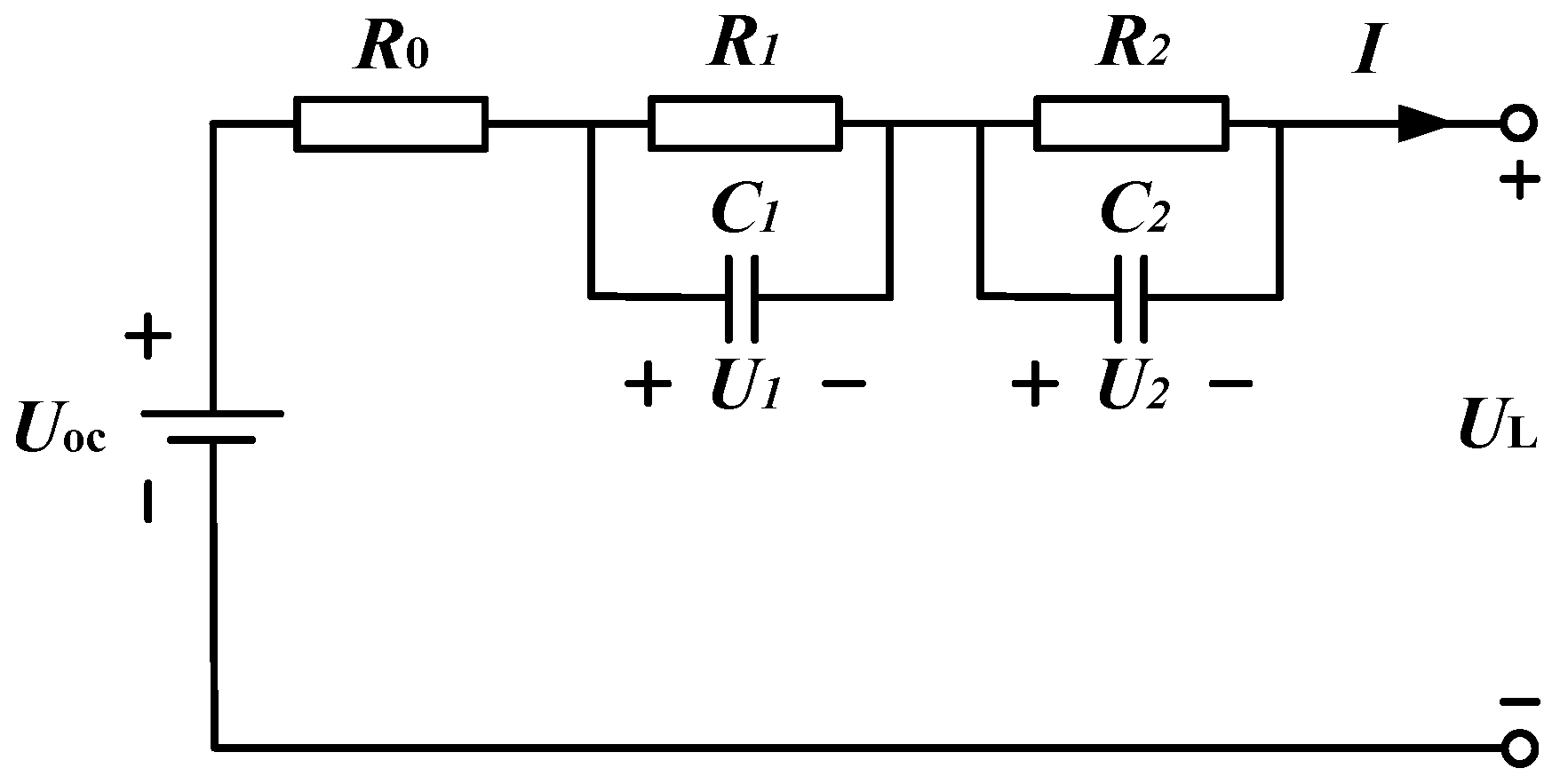
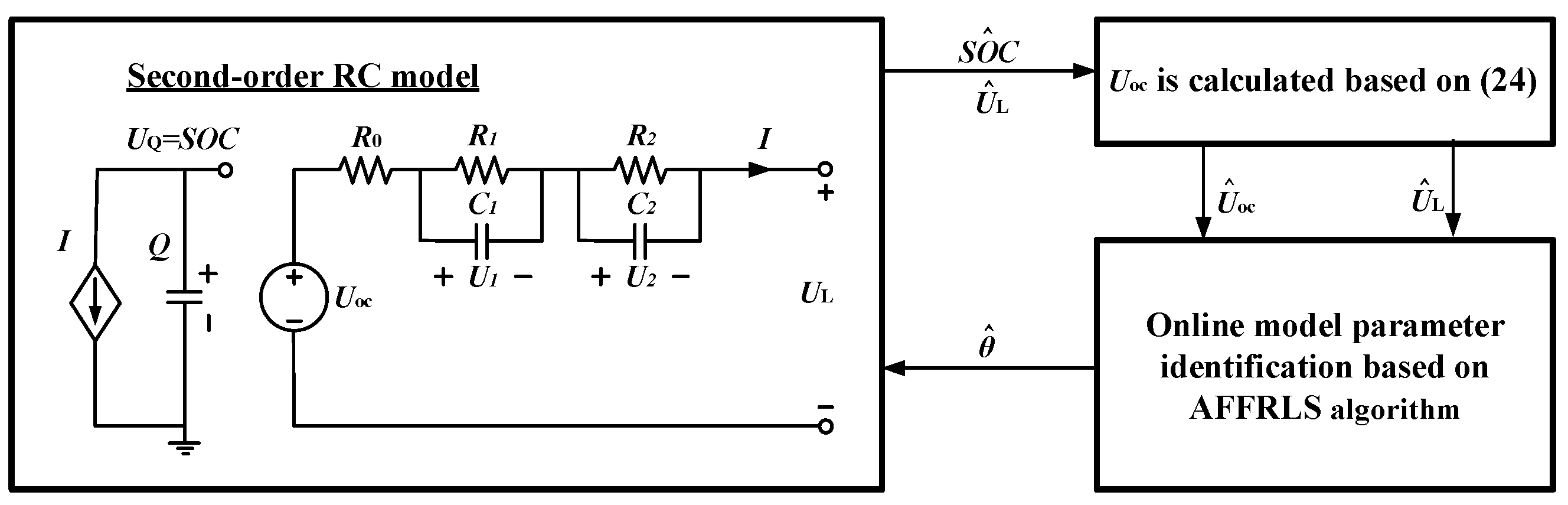
2. Lithium-Ion Battery Modeling

The second-order RC equivalent circuit model of a lithium-ion battery is shown in Figure 1. It consists of an ideal voltage source U_oc, ohmic resistor R₀, and two RC parallel circuits. U_oc represents the open circuit voltage of the lithium battery. R₀ indicates the internal resistance of the battery. The two RC parallel circuits represent the electrochemical polarization and concentration polarization effects in the battery reactions. U_L is the battery terminal voltage. The following is the analysis process of the equivalent circuit model shown in Figure 1 [13,14,15]. According to Kirchhoff’s voltage law and current law, the electrical characteristic equation of the model is expressed by (1).

$$\begin{array}{l}{U}_L=U_{oc}[SOC(t)]-U_1-U_2-I(t)\cdot R_0\\ C_1\cdot \frac{d{U}_1}{dt}=I(t)-\frac{U_1}{R_1}\\ C_2\cdot \frac{d{U}_2}{dt}=I(t)-\frac{U_2}{R_2}\end{array}$$

(1)

Equation (1) is written as a frequency domain expression.

$$E=U_L(s)-U_{oc}(s)=-I(s)\left(R_0+\frac{R_1}{1+R_1{C}_{1}s}+\frac{R_2}{1+R_2{C}_{2}s}\right)$$

(2)

Equation (2) is rewritten to (3).

$$G(s)=\frac{E(s)}{I(s)}=-\frac{R_0{s}^2+\frac{R_0{R}_1{C}_1+R_0{R}_2{C}_2+R_2{R}_1{C}_1+R_1{R}_2{C}_2}{R_1{C}_1{R}_2{C}_2}s+\frac{R_0+R_1+R_2}{R_1{C}_1{R}_2{C}_2}}{s^2+\frac{R_1{C}_1+R_2{C}_2}{R_1{C}_1{R}_2{C}_2}s+\frac{1}{R_1{C}_1{R}_2{C}_2}}$$

(3)

Bilinear transformation $s=\frac{2}{T}\cdot \frac{1-z^{-1}}{1+z^{-1}}$ is brought into (3), and Equations (4) and (5) are obtained.

$$G(z^{-1})=\frac{E(k)}{I(k)}=\frac{{\theta }_3+{\theta }_4{z}^{-1}+{\theta }_5{z}^{-2}}{1-{\theta }_1{z}^{-1}-{\theta }_2{z}^{-2}}$$

(4)

$$\{\begin{array}{l}{\theta }_1=\frac{2T^2-8R_1{C}_1{R}_2{C}_2}{-T^2-2T(R_1{C}_1+R_2{C}_2)-4R_1{C}_1{R}_2{C}_2}\\ {\theta }_2=\frac{T^2-2T(R_1{C}_1+R_2{C}_2)+4R_1{C}_1{R}_2{C}_2}{-T^2-2T(R_1{C}_1+R_2{C}_2)-4R_1{C}_1{R}_2{C}_2}\\ {\theta }_3=\frac{T^2(R_0+R_1+R_2)+2T(R_0{R}_1{C}_1+R_0{R}_2{C}_2+R_1{R}_2{C}_2+R_2{R}_1{C}_1)+4R_0{R}_1{C}_1{R}_2{C}_2}{-T^2-2T(R_1{C}_1+R_2{C}_2)-4R_1{C}_1{R}_2{C}_2}\\ {\theta }_4=\frac{2T^2(R_0+R_1+R_2)-8R_0{R}_1{C}_1{R}_2{C}_2}{-T^2-2T(R_1{C}_1+R_2{C}_2)-4R_1{C}_1{R}_2{C}_2}\\ {\theta }_5=\frac{T^2(R_0+R_1+R_2)-2T(R_0{R}_1{C}_1+R_0{R}_2{C}_2+R_1{R}_2{C}_2+R_2{R}_1{C}_1)+4R_0{R}_1{C}_1{R}_2{C}_2}{-T^2-2T(R_1{C}_1+R_2{C}_2)-4R_1{C}_1{R}_2{C}_2}\end{array}$$

(5)

Therefore, the recursive Equation (6) is obtained by (4).

$$E(k)={\theta }_{1}E(k-1)+{\theta }_{2}E(k-2)+{\theta }_{3}I(k)+{\theta }_{4}I(k-1)+{\theta }_{5}I(k-2)$$

(6)

where E(k − 1) and E(k − 2) are the difference between the terminal voltage and the open circuit voltage at the time of k − 1 and k − 2. I(k), I(k − 1), and I(k − 2) are input currents at the time of k, k − 1, and k − 2.

Suppose that a, b, c, d, f are represented by (7).

$$\{\begin{array}{l}a=R_0\\ b=R_1{C}_1{R}_2{C}_2\\ c=R_1{C}_1+R_2{C}_2\\ d=R_0+R_1+R_2\\ f=R_0{R}_1{C}_1+R_0{R}_2{C}_2+R_1{R}_2{C}_2+R_2{R}_1{C}_1\end{array}$$

(7)

Equation (7) is brought into (5) and simplified to (8).

$$\{\begin{array}{l}{\theta }_1=\frac{8b-2T^2}{4b+2cT+T^2}\\ {\theta }_2=\frac{4cT}{4b+2cT+T^2}-1\\ {\theta }_3=-\frac{4ab+2eT+d{T}^2}{4b+2cT+T^2}\\ {\theta }_4=\frac{8ab-2d{T}^2}{4b+2cT+T^2}\\ {\theta }_5=-\frac{4ab-2eT+d{T}^2}{4b+2cT+T^2}\end{array}$$

(8)

Therefore, Equation (9) is obtained by (8).

$$\{\begin{array}{l}a=\frac{{\theta }_4-{\theta }_3-{\theta }_5}{1+{\theta }_1-{\theta }_2}\\ b=\frac{T^2(1+{\theta }_1-{\theta }_2)}{4(1-{\theta }_1-{\theta }_2)}\\ c=\frac{T(1+{\theta }_2)}{1-{\theta }_1-{\theta }_2}\\ d=\frac{-{\theta }_3-{\theta }_4-{\theta }_5}{1-{\theta }_1-{\theta }_2}\\ f=\frac{T({\theta }_5-{\theta }_3)}{1-{\theta }_1-{\theta }_2}\end{array}$$

(9)

where T is the sampling time.

Suppose ${\tau }_1=\frac{c+\sqrt{c^2-4b}}{2},{\tau }_2=\frac{c-\sqrt{c^2-4b}}{2}$. Thus, the resistance and capacitance parameters $R_0$, $R_1$, $R_2$, $C_1$, and $C_2$ can be obtained by (10).

$$\{\begin{array}{l}{R}_0=a\\ R_1=[{\tau }_1(d-a)+ac-f]/({\tau }_1-{\tau }_2)\\ R_2=d-a-R_1\\ C_1={\tau }_1/R_1\\ C_2={\tau }_2/R_2\end{array}$$

(10)

3. Online Parameter Identification Principle

3.1. Forgetting Factor Recursive Least Square Method

The RLS method is the most commonly used method for system parameter identification [19]. This method uses the square norm of the discrete function as a metric to get the identification parameters. Equation (11) can be obtained from (6) when the system error is considered. It is a discrete expression of the system to be identified.

$$E(k)={\theta }_{1}E(k-1)+{\theta }_{2}E(k-2)+{\theta }_{3}I(k)+{\theta }_{4}I(k-1)+{\theta }_{5}I(k-2)+e(k)$$

(11)

Define the parameter vector $\mathit{\theta }$ and the observation data matrix $\mathit{\phi }$ as follows:

$$\theta ={[{\theta }_1\hspace{1em}{\theta }_2\hspace{1em}{\theta }_3\hspace{1em}{\theta }_4\hspace{1em}{\theta }_5]}^T$$

(12)

$$\phi =\left[\begin{array}{ccccc}E(k-1)& E(k-2)& I(k)& I(k-1)& I(k-2)\\ E(k-2)& E(k-3)& I(k-1)& I(k-2)& I(k-3)\\ & & ⋮& & \\ E(k-m-1)& E(k-m-2)& I(k-m)& I(k-m-1)& I(k-m-2)\end{array}\right]$$

(13)

where k denotes the current moment. m is the observation times. $\mathit{\phi }$ is the known observation data matrix. $\mathit{\theta }$ is the parameter vector to be estimated. The matrix form of (11) can be expressed from (12) and (13).

$$E=\phi \theta +e$$

(14)

where e is the systematic error vector $e={[e(k)\hspace{1em}e(k-1)\hspace{1em}\cdots \hspace{1em}e(k-m)]}^T$. E is the system output vector, and its data is the observation value of system output $E={[E(k)\hspace{1em}E(k-1)\hspace{1em}\cdots \hspace{1em}E(k-m)]}^T$. The evaluation function of the RLS method is given by (15).

$$J={\displaystyle \sum _{t=0}^m{[e(k-t)]}^2=e^{T}e}$$

(15)

If the derivative of J is zero, the parameter vector ${\mathit{\theta }}^{\prime }$ can be obtained in the smallest case of (14).

$$\begin{array}{c}{\frac{\partial J}{\partial \theta }|}_{\theta ={\theta }^{\prime }}=\frac{\partial J}{\partial \theta }\left[{(E-\phi \theta )}^T(E-\phi \theta )\right]=0\\ {\phi }^{T}E={\phi }^T\phi {\theta }^{\prime }\end{array}$$

(16)

When ${\mathit{\phi }}^{\mathbf{T}}\mathit{\phi }$ is a full rank matrix, the parameter estimation of the RLS method is expressed by (17).

$${\theta }^{\prime }={({\phi }^T\phi )}^{-1}{\phi }^{T}E$$

(17)

On the basis of the RLS method, the FFRLS method is to add the forgetting factor $\lambda$ as a coefficient in the observed data matrix φ and the system output vector E, they are expressed by (18) and (19). When each observation obtains new data, the proportion of new and old data is adjusted by exponential weighting, and then the last obtained identification parameter is corrected. Thus, when the input variables change, the FFRLS method can respond quickly and obtain better identification parameters as the system observation data increase.

$$E={[E(k)\hspace{1em}\lambda E(k-1)\hspace{1em}\cdots \hspace{1em}{\lambda }^{m}E(k-m)]}^T$$

(18)

$$\phi =\left[\begin{array}{ccccc}E(k-1)& E(k-2)& I(k)& I(k-1)& I(k-2)\\ \lambda E(k-2)& \lambda E(k-3)& \lambda I(k-1)& \lambda I(k-2)& \lambda I(k-3)\\ & & ⋮& & \\ {\lambda }^{m}E(k-m-1)& {\lambda }^{m}E(k-m-2)& {\lambda }^{m}I(k-m)& {\lambda }^{m}I(k-m-1)& {\lambda }^{m}I(k-m-2)\end{array}\right]$$

(19)

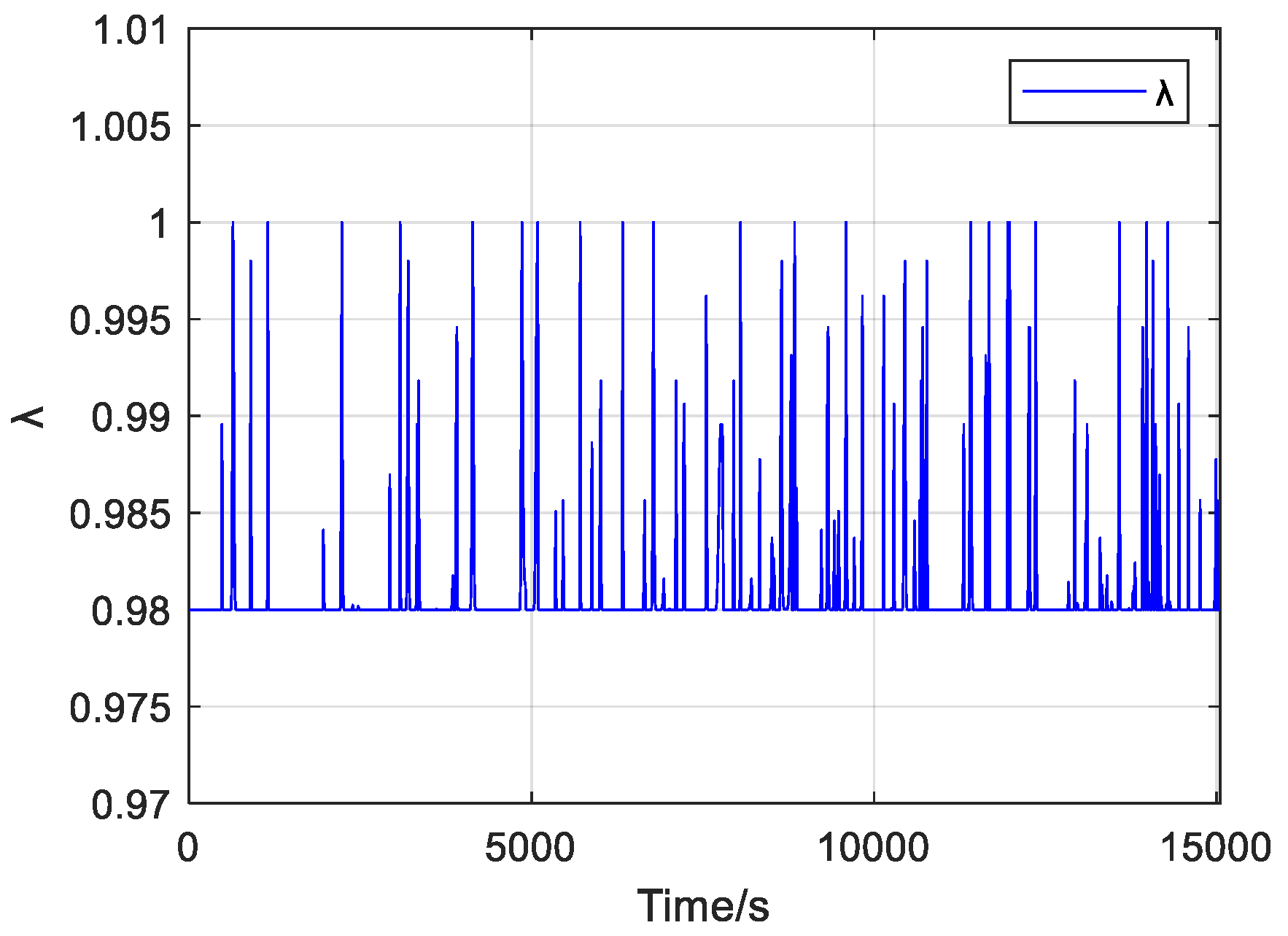
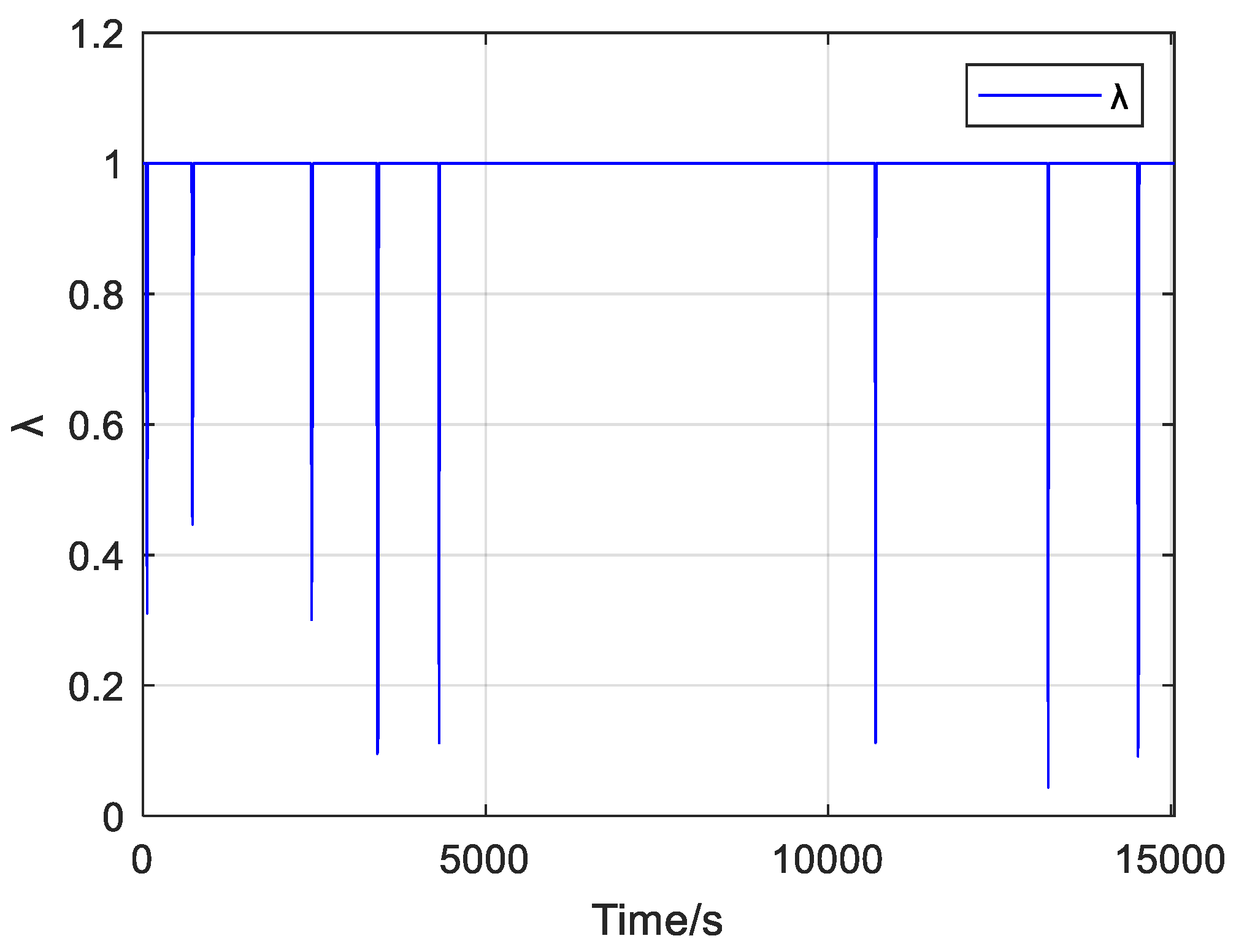
3.2. Adaptive Forgetting Factor Analysis

$\lambda$ allocates the weights of old and new data, and usually takes a constant of 0.98. When $\lambda =1$, the FFRLS method degenerates into the RLS method. Since the forgetting factor is constant, when the online identification parameter error is very small, the introduction of the forgetting factor may increase the online identification parameter error. When the online identification parameter error is very large, it is desirable to optimize the forgetting factor to make the online identification have faster convergence speed and reduce the identification error. Therefore, it is expected that the forgetting factor can vary adaptively with the identification parameter error.

The most critical part of the variable forgetting factor least squares algorithm (VFFRLS) is how to make the forgetting factor adaptively change. In the steady state, the forgetting factor $\lambda$ is close to or equal to 1. On the contrary, the forgetting factor $\lambda$ tends to be a suitable value, which only affects the error of the nearby moment, so that the online identification parameter can be quickly tracked to the actual value, and $\lambda$ is gradually increased to the optimum value at steady state. An equation for calculating the adaptive forgetting factor is proposed to achieve the above purpose, it is expressed by (20).

$$\begin{array}{l}\lambda (k)={\lambda }_{\min }+(1-{\lambda }_{\min })\cdot h^{\epsilon (k)}\\ \epsilon (k)=round({(\frac{e(k)}{e_{base}})}^2)\end{array}$$

(20)

where ${\lambda }_{\min }$ is the minimum value of the forgetting factor. Usually, the range of forgetting factor is 0.95~1 [15,20] and it is found by the experimental data that the equivalent circuit model parameters identified by the AFFRLS algorithm are accurate and fast as the range of forgetting factor is selected as 0.98~1, and, therefore, ${\lambda }_{\min }$ is 0.98. h is the sensitivity coefficient. h may be selected as any value between 0 and 1, which indicates the sensitivity of forgetting factor to the errors. When h is close to 1 (e.g., 0.99), the forgetting factor changes slowly from 1 to 0.98, which leads to the slow response speed of parameter identification. Conversely, when h is close to 0 (e.g., 0.01), the forgetting factor quickly changes from 1 to 0.98, which results in the response speed of parameter identification too fast and reduces the accuracy. Therefore, h is generally chosen to be 0.9, which takes into account the balance between the rapidity and accuracy of identification parameters. e(k) is the error at k time and $e_{base}$ is the allowable error reference. Equation (20) shows that the forgetting factor $\lambda$ decreases rapidly when the kth error e(k) exceeds $e_{base}$; hence, $e_{base}$ is usually chosen according to the magnitude of the expected error. When the identification parameter error is less than $e_{base}$, the identification parameters are considered stable and $\lambda$ changes to a larger value. When the error of identification parameters is greater than $e_{base}$, the identification parameters are considered unstable and the change of $e_{base}$ is smaller. The function $round\left(n\right)$ represents the integer closest to n. It can be seen from (20) that the larger the error value, the smaller the forgetting factor $e_{base}$, and its variation range is between 0.98 and 1; thus, the forgetting factor can be adaptively changed with the error of identification parameters.

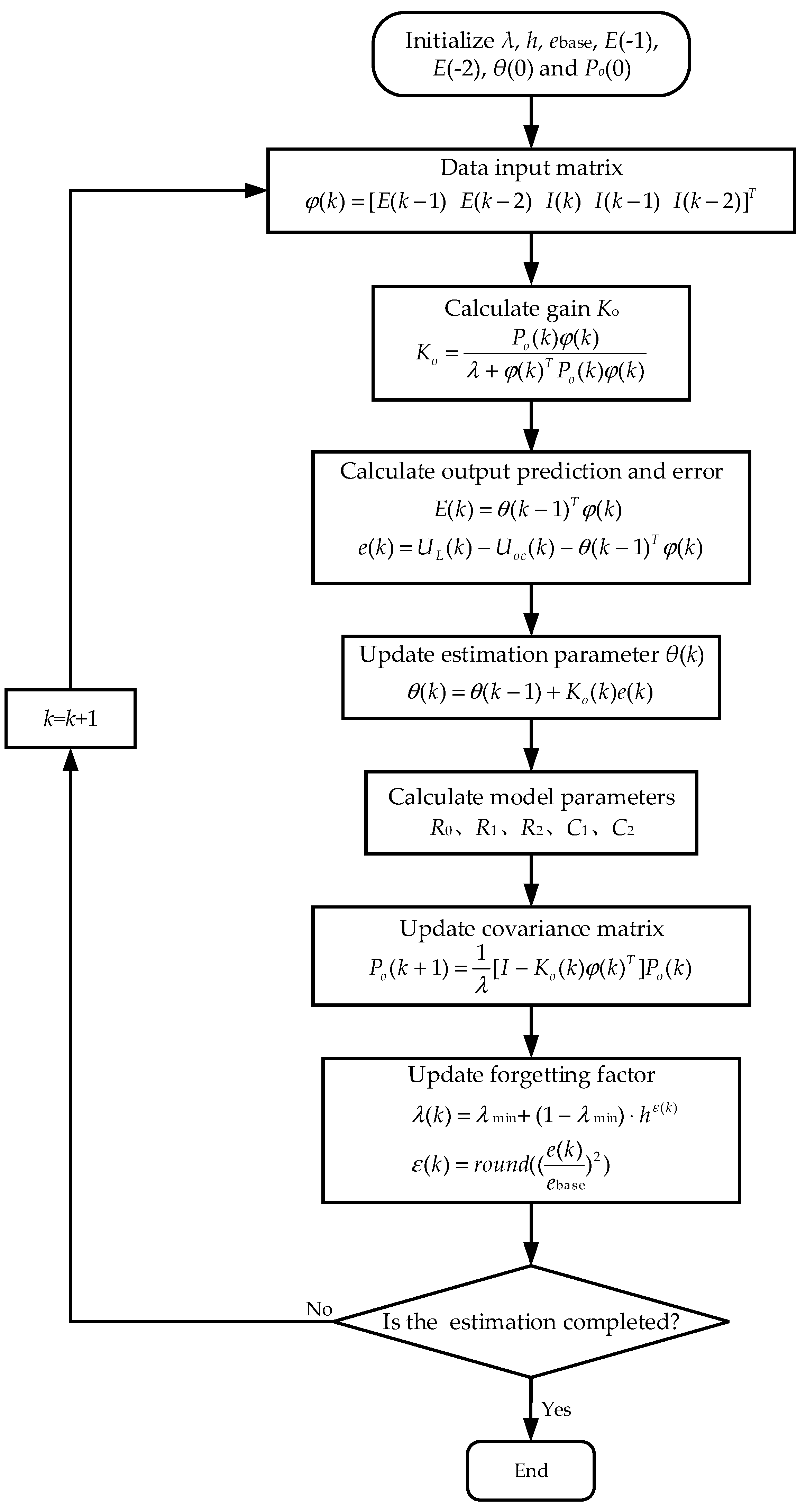
3.3. Implementation of Online Parameter Identification Algorithm Based on AFFRLS

It is seen from the above analysis that each parameter in the second-order RC equivalent circuit model of the lithium-ion battery can be calculated by (10) as long as θ₁, θ₂, θ₃, θ₄, and θ₅ in (4) are estimated. Therefore, it is necessary to identify θ₁, θ₂, θ₃, θ₄, and θ₅ by using the online parameter identification algorithm based on AFFRLS. The overall block diagram is shown in Figure 2. The specific implementation flow chart of AFFRLS is shown in Figure 3.

The online parameter identification algorithm is performed by the AFFRLS. It is known from (12) and (13) that $\theta (k)={[{\theta }_1\hspace{1em}{\theta }_2\hspace{1em}{\theta }_3\hspace{1em}{\theta }_4\hspace{1em}{\theta }_5]}^T$ and $\phi (k)={[E(k-1)\hspace{1em}E(k-2)\hspace{1em}I(k)\hspace{1em}I(k-1)\hspace{1em}I(k-2)]}^T$. Where $\phi (k)$ is the known data at time k, and $\theta (k)$ is the parameter to be estimated at time k.

The given initial value $\theta \left(0\right)$ generally is a sufficiently small real matrix. At the two moments before the start of the algorithm, the input current is zero, and the open circuit voltage U_oc is equal to the terminal voltage U_L, so $E(-1)=E(-2)=0$, and the initial $\varphi \left(0\right)$ value is [0 0 0 0 0]. The gain matrix K_o is calculated by (21) [14].

$$K_o=\frac{P_o(k-1)\phi (k)}{\lambda +\phi {(k)}^T{P}_o(k-1)\phi (k)}$$

(21)

where $P_o\left(k\right)$ is the covariance matrix at time k and its initial value is an identity matrix.

Hence, the estimated parameter $\theta \left(k\right)$ is updated by (22).

$$\theta (k)=\theta (k-1)+K_o(k)[U_L(k)-U_{oc}(k)-\theta {(k-1)}^T\phi (k)]$$

(22)

where the open circuit voltage $U_{oc}\left(k\right)$ at time k is given by the polynomial between the open circuit voltage (OCV) and the SOC.

$\lambda$ is obtained from (20) and taken into (21) to obtain the gain matrix K_o. Bringing K_o into (22) and θ₁, θ₂, θ₃, θ₄, and θ₅ are obtained. The estimated values of $R_0$, $R_1$, $R_2$, $C_1$, and $C_2$ at time k can then be obtained by (9) and (10).

According to (23), the covariance matrix $P_o(k)$ is updated by the obtained gain matrix K_o. The parameter identification at the next moment is performed again. Where I is an identity matrix.

$$P_o(k)=\frac{1}{\lambda }[I-K_o(k)\phi {(k)}^T]P_o(k-1)$$

(23)

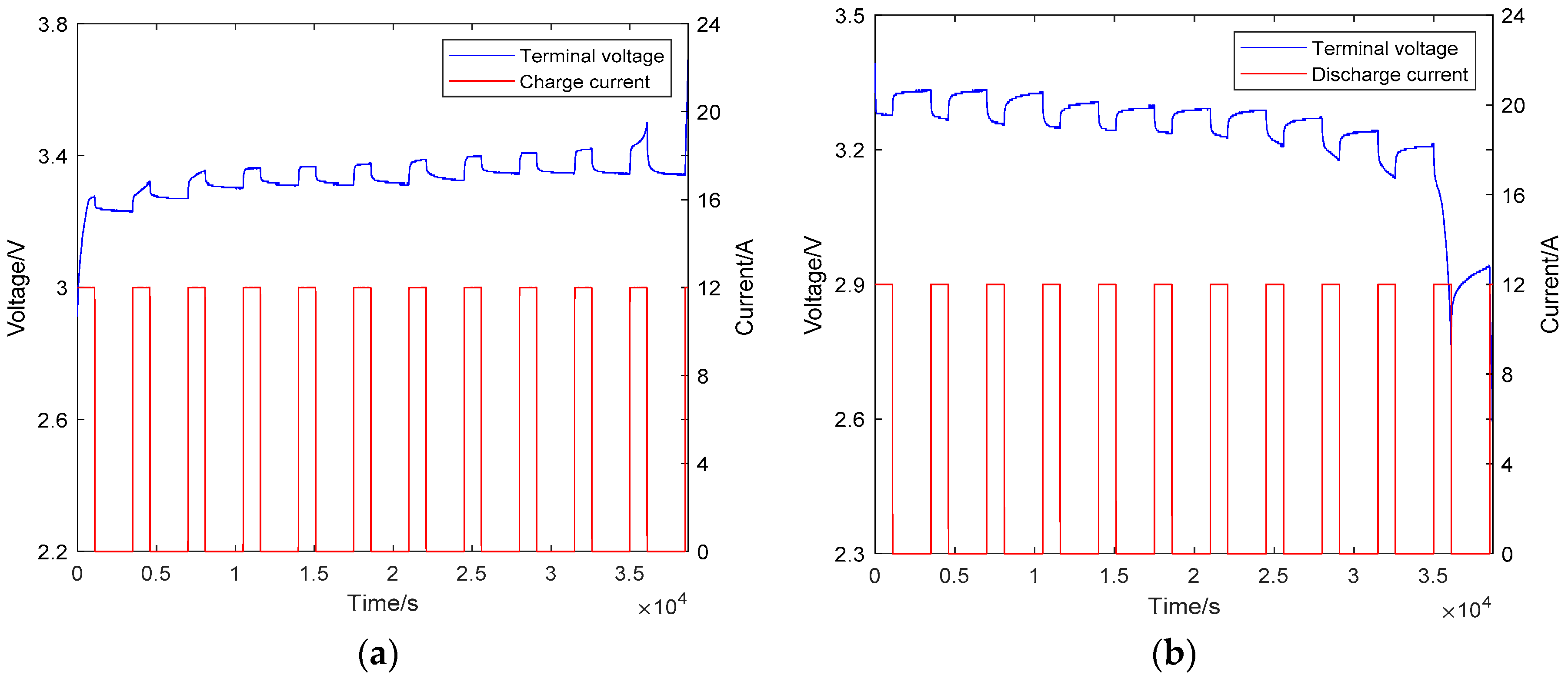
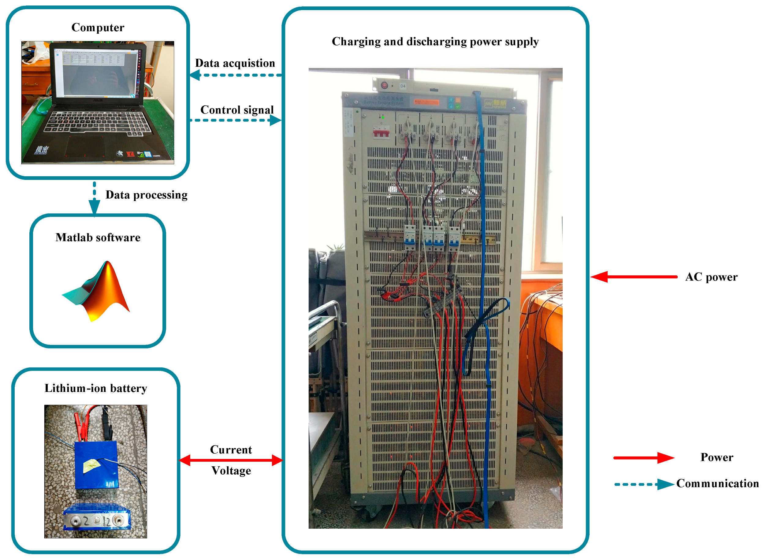
4. Experimental Verification and Analysis

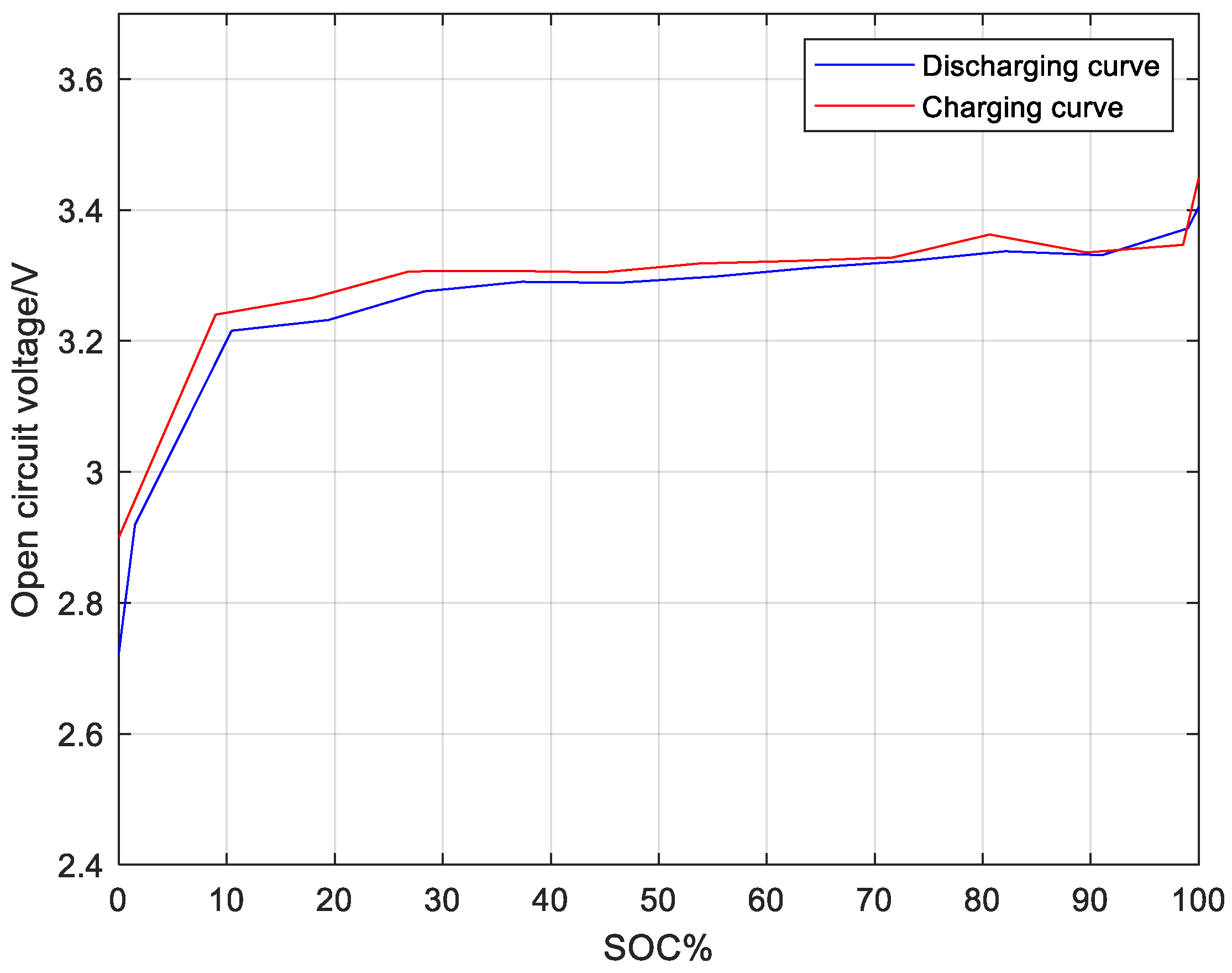
The special power supply is used to charge and discharge the 3.2 V/36 Ah lithium iron phosphate battery produced by Shandong Wina Green Power Co., Ltd in Weifang, China. The sampling time is T = 10 s and the environment temperature is 25 °C. The experimental platform and the specification of the battery are shown in Figure 4 and

Table 1. The battery specifications.

Parameter	Value
Rated capacity (Ah)	36
Nominal voltage (V)	3.2
Standard charging/discharging current (A)	12
Charging cut-off voltage (V)	3.7
Discharging cut-off voltage (V)	2.5
Maximum continuous discharging current (A)	108

, respectively.

4.1. OCV-SOC Curve

Intermittent constant current charging and discharging experiments with 0.33 C standard rate current recommended by a company are carried out. The charging and discharging experimental curves are shown in Figure 5, and the obtained SOC-OCV data are given by

Table 2. The state of charge (SOC)-open circuit voltage (OCV) data.

Item	1	2	3	4	5	6	7	8	9	10	11	12	13
Intermittent constant current charging experiments with 0.33 C standard current
SOC/%	0	8.96	17.92	26.88	35.84	44.80	53.76	62.72	71.68	80.64	89.60	98.56	100
OCV/V	2.902	3.233	3.270	3.304	3.311	3.311	3.311	3.326	3.344	3.348	3.344	3.341	3.615
Intermittent constant current discharging experiments with 0.33 C standard current
SOC/%	0	1.49	10.45	19.40	28.36	37.31	46.27	55.22	64.18	73.13	82.09	91.04	100
OCV/V	2.683	2.939	3.214	3.244	3.270	3.289	3.292	3.300	3.307	3.330	3.333	3.333	3.393

. Polynomial fitting of the experimental data is performed by using Matlab software, Equation (24) is obtained, which provides an open circuit voltage U_oc for the FFRLS or AFFRLS algorithm. The OCV-SOC relationship curve under this condition is shown in Figure 6. It is seen from Figure 6 that the OCV-SOC curve of the entire charging and discharging process is approximately a hysteresis curve. Therefore, the influence of the charging and discharging current direction on the open circuit voltage needs to be considered during the online parameter identification.

$$\begin{array}{l}{U}_{ocDis}=1813.4*SO{C}^9-8629.9*SO{C}^8+17470*SO{C}^7-19595*SO{C}^6\\ \hspace{1em}\hspace{1em}+13285*SO{C}^5-5570.7*SO{C}^4+1419.9*SO{C}^3-208.1*SO{C}^2\\ \hspace{1em}\hspace{1em}+15.953*SOC+2.7228\\ U_{ocCha}=3060.5*SO{C}^9-13713*SO{C}^8+25909*SO{C}^7-26862*SO{C}^6\\ \hspace{1em}\hspace{1em}+16655*SO{C}^5-6310.9*SO{C}^4+1434.4*SO{C}^3-185.1*SO{C}^2\\ \hspace{1em}\hspace{1em}+12.471*SOC+2.9002\end{array}$$

(24)

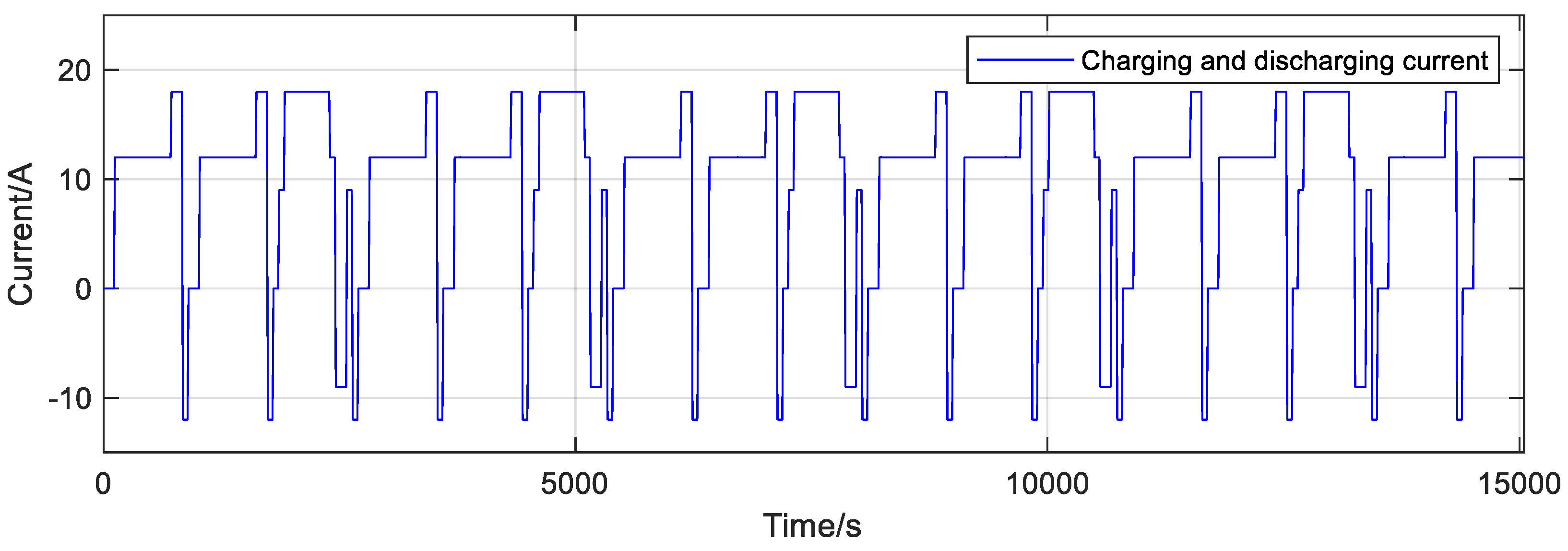
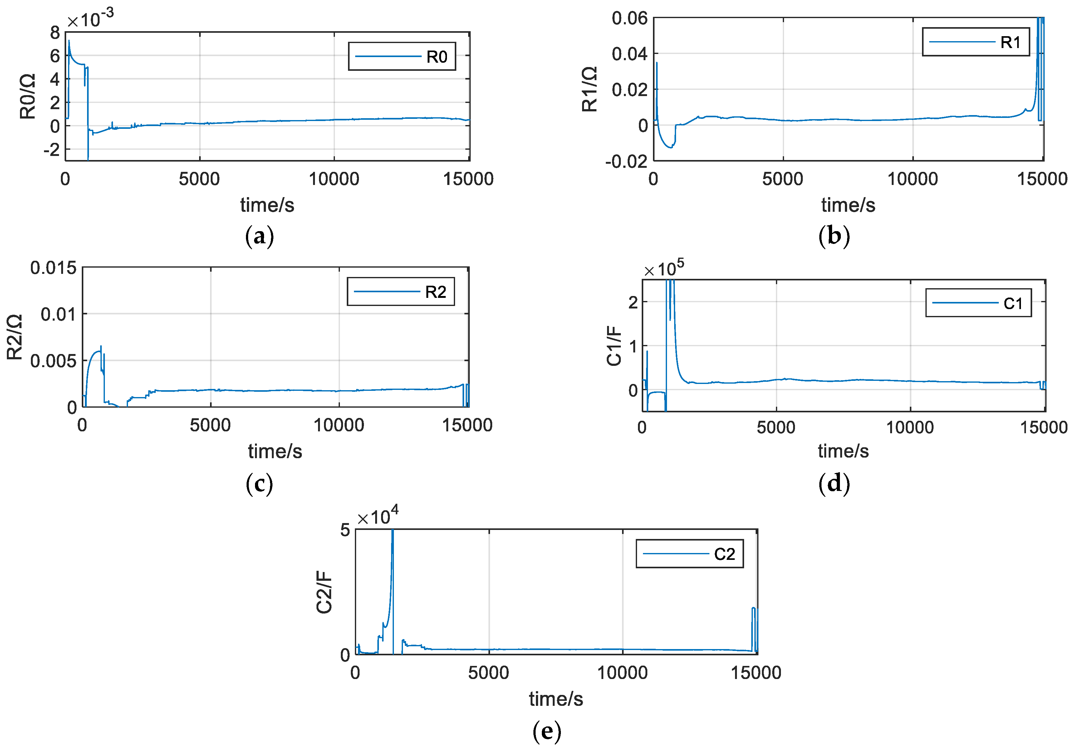
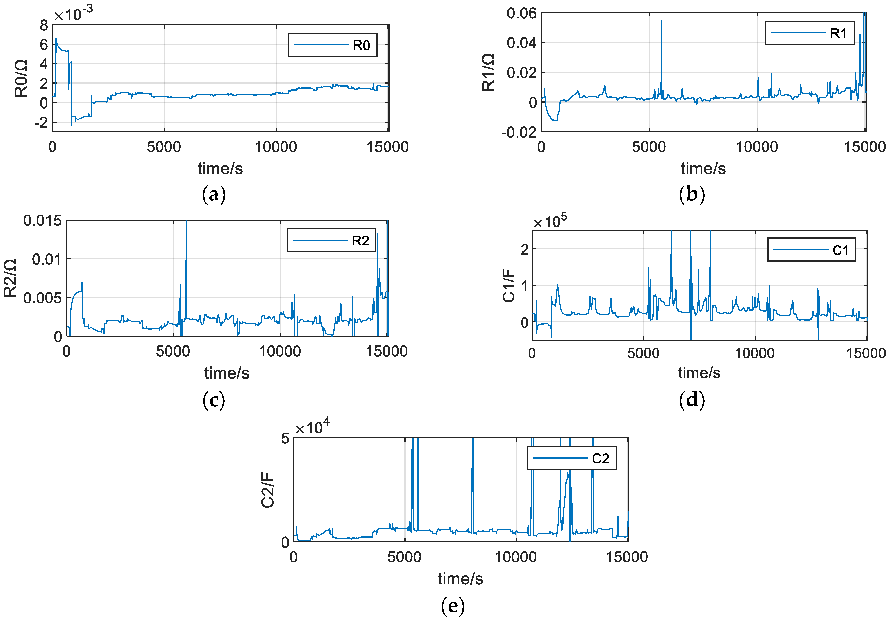
4.2. Online Parameter Identification of Lithium-Ion Battery Equivalent Model

The dynamic stress test (DST) experiment has a strict charge and discharge process, it is shown in Figure 7. The cyclic charge current rates are 0.22 C, 0.33 C, and 0.5 C, and the cyclic discharge current rates are 0.22 C and 0.33 C, respectively. Under these conditions, the validity of the online parameter identification algorithm can be more rigorously verified.

Figure 8 and Figure 9 are the identified parameter curves of the FFRLS algorithm and the AFFRLS algorithm under the DST conditions, respectively. Comparing Figure 8 and Figure 9, it can be seen that the parameters identified by the FFRLS algorithm are relatively stable, but the identification ability of dynamic parameter change is insufficient. The parameters identified by the AFFRLS algorithm have obvious fluctuations, which more accurately reflect the complex characteristics of real-time variation of each parameter with the change of charging and discharging current. The dynamic parameters also have more spikes, which fully highlights the identification ability when charging and discharging currents are frequently switched. Figure 10 shows the adaptive forgetting factor λ. It can be seen that the forgetting factor $\lambda$ has many spikes. And it is adaptively varied with the change of charging and discharging current, which is beneficial to enhance the dynamic parameter identification ability of the AFFRLS algorithm.

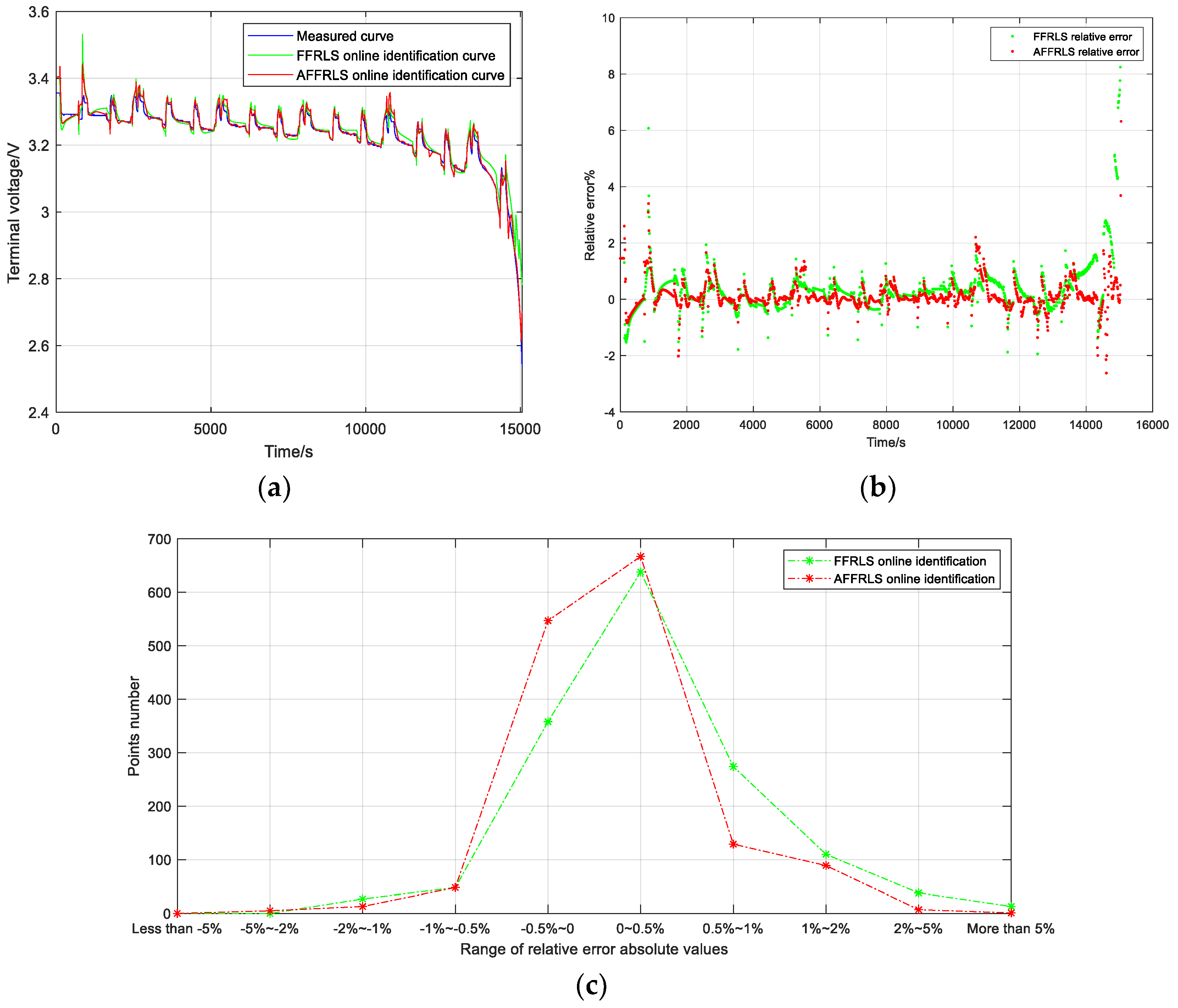
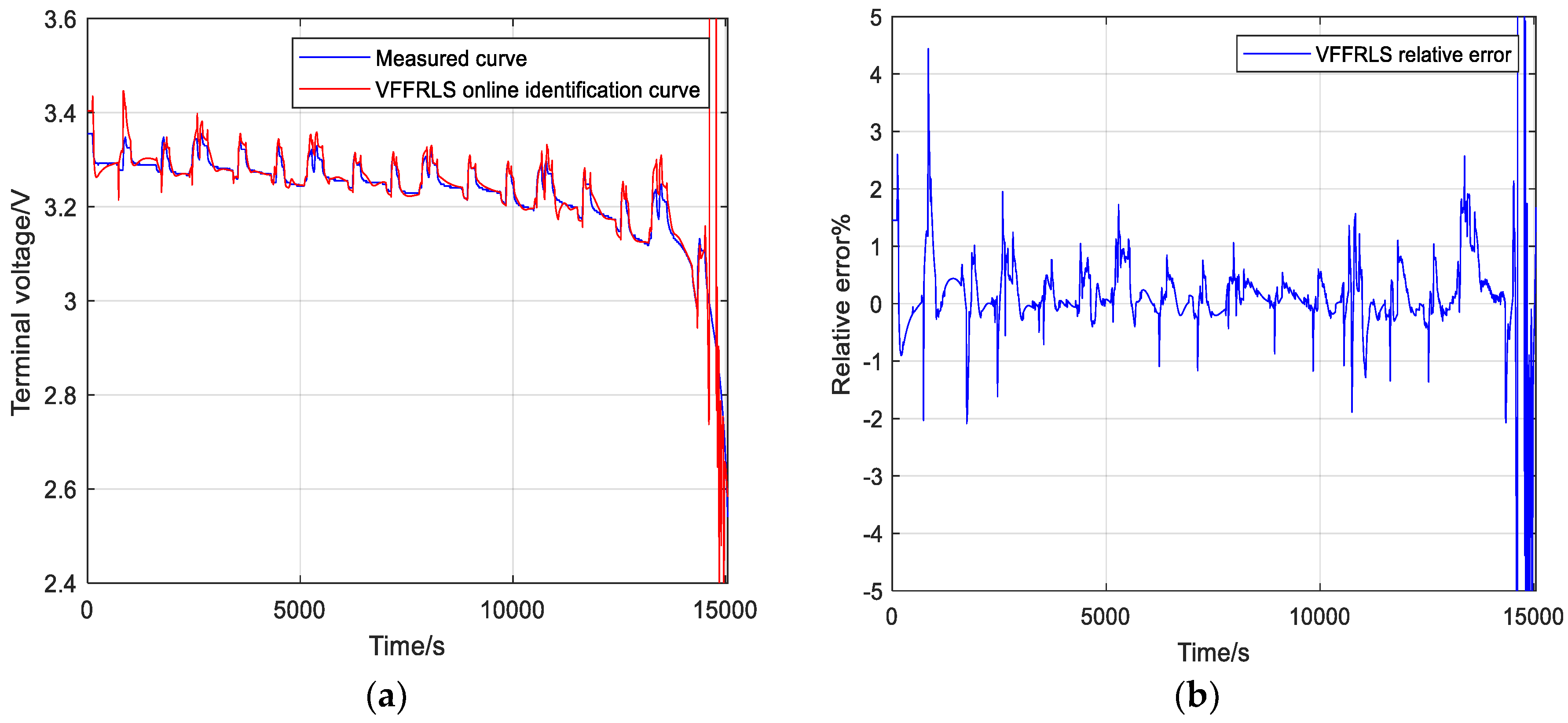
4.3. Comparative Analysis of the Prediction Effect of the Lithium-Ion Battery Terminal Voltage

The experimental conditions in Figure 11 and Figure 12 are the same as those in Figure 7. The FFRLS algorithm and the AFFRLS algorithm are used to predict the lithium-ion battery terminal voltage respectively on the basis of the identification parameters shown in Figure 8 and Figure 9, and Figure 11 is a comparison of the measured terminal voltage and the terminal voltage identified by the FFRLS and AFFRLS algorithms. Figure 12 is a comparison of the measured terminal voltage and the terminal voltage identified by the VFFRLS algorithm of literature [16] with a certain weight coefficient. It may be determined from Figure 11 and Figure 12 which algorithm identifies the circuit parameters more accurately and responds faster.

Figure 11a is the measured terminal voltage and the terminal voltage identified by the FFRLS and AFFRLS algorithms. Figure 11b shows the scatter plot of relative error for FFRLS and AFFRLS algorithms. The range of absolute value of relative errors in Figure 11b is divided into 10 intervals, and the points of relative errors falling into each interval are counted, and Figure 11c is obtained. As can be seen from Figure 11c, the relative error distribution of AFFRLS in the range of (±0.5%) is significantly higher than that of FFRLS, while the relative error distribution in other ranges is mostly lower than that of FFRLS.

From the aspect of the sample average and standard deviation, sample average value of the relative errors is 0.372% and sample standard deviation of the relative errors is 0.947 for FFRLS. The AFFRLS sample average value is 0.136%, and the sample standard deviation is 0.526. The sample average and standard deviation of AFFRLS algorithm are smaller than those of FFRLS algorithm.

The FFRLS algorithm and AFFRLS algorithm are tested by F-test. Assume H₀: There is no significant difference in the total variance between the two algorithms. H₁: There is a significant difference in the total variance between the two algorithms. Significance level is set to 0.05 and tail type is bilateral, H = 1, p = 3.9233 × 10⁻¹⁰⁹ is obtained. The confidence interval of mean difference is [2.9293, 3.5856], and we can see from H = 1, p = 3.9233 × 10⁻¹⁰⁹ < 0.05 that the original hypothesis is not accepted, i.e., there is a significant difference in variance between the two algorithms.

The FFRLS algorithm and AFFRLS algorithm are tested by t-test. Assume H₀: There is no significant difference in the average value of the two algorithms. H₁: There is a significant difference in the average value of the two algorithms. The significance level is 0.05, the tail type is bilateral, and the variance type is unequal. H = 1, p = 3.9716 × 10⁻¹⁷ is obtained, the confidence interval of mean difference is [0.18189, 0.29135]. We can see from H = 1, p = 3.9716 × 10⁻¹⁷ < 0.05 that the original hypothesis is not accepted, i.e., there is a significant difference in the average value between the two algorithms.

In summary, the average value of AFFRLS algorithm is closer to zero than that of FFRLS algorithm, and the variance is smaller, which shows that the parameter identification result of AFFRLS algorithm is more accurate than that of FFRLS algorithm.

Figure 13 is a real-time variation curve of the forgetting factor obtained by the algorithm of literature [16] under a certain weight coefficient. It can be seen from Figure 12 that this algorithm also has a good terminal voltage prediction capability, but it is more demanding on the weight coefficient. When the weight coefficient is not appropriate, the forgetting factor will be too small and the parameter changes drastically, which may lead to the divergence of the algorithm. While the AFFRLS algorithm in this paper limits the variation range of the forgetting factor, it has better stability and the range of correlation coefficients is more relaxed.

The VFFRLS algorithm of the literature [16] to be compared is written into the same program together with the AFFRLS algorithm proposed in this paper. The two algorithms run in parallel and measure the computing time corresponding to each experimental data respectively. Last, the total computing time of the two algorithms is obtained by accumulating the computing time, respectively. The average calculation time of the AFFRLS algorithm in this paper is 17.65 ms, and that of the literature [16] is 26.05 ms. The average calculation time is saved by 32.25%. This indicates that the adaptive algorithm of this paper is simpler, the operation time is shorter, and the real-time performance is better, which is beneficial to the practical application of the algorithm in the micro-controller such as digital signal processor (DSP).

5. Conclusions

In this paper, the second-order RC equivalent circuit model of the lithium-ion battery is analyzed, and the online identification algorithm of the equivalent circuit model parameters based on the AFFRLS is studied. The correctness of the equivalent circuit model parameter identification in the case of charging and discharging is verified by the DST experiment, and the prediction terminal voltage obtained by the model parameters are compared with the actual terminal voltage. The experimental results show that the proposed AFFRLS algorithm has a more accurate parameter identification ability than the original FFRLS algorithm. Compared with other VFFRLS algorithms, it has better stability of parameter identification and shorter operation time.

References

1. Hannan, M.A.; Hoque, M.M.; Hussain, A.; Yusof, Y.; Ker, P.J. State-of-the-art and energy management system of lithium-ion batteries in electric vehicle applications: Issues and recommendations. IEEE Access 2018, 6, 19362–19378. [Google Scholar] [CrossRef]
2. Xu, J.; Mi, C.C.; Cao, B.; Deng, J.; Chen, Z.; Li, S. The state of charge estimation of lithium-ion batteries based on a proportional-integral observer. IEEE Trans. Veh. Technol. 2014, 63, 1614–1621. [Google Scholar]
3. Paschero, M.; Storti, G.L.; Rizzi, A.; Mascioli, F.M.F.; Rizzoni, G. A novel mechanical analogy based battery model for SoC estimation using a multi-cell EKF. IEEE Trans. Sustain. Energy 2016, 7, 1695–1702. [Google Scholar] [CrossRef]
4. Zhang, Z.L.; Cheng, X.; Lu, Z.Y.; Gu, D.J. SOC estimation of lithium-ion batteries with AEKF and wavelet transform matrix. IEEE Trans. Power Electron. 2017, 32, 7626–7634. [Google Scholar] [CrossRef]
5. Hardik, K.; Jesse, T.; Taha, S.U. Comparison of lead-acid and lithium ion batteries for stationary storage in off-grid energy systems. In Proceedings of the 4th IET Clean Energy and Technology Conference (CEAT 2016), Kuala Lumpur, Malaysia, 14–15 November 2016; pp. 1–7. [Google Scholar]
6. Daniel, R.; Alfredo, P.; Marco, R.; Michele, O. 12V battery modeling: Model development, simulation and validation. In Proceedings of the 2017 International Conference of Electrical and Electronic Technologies for Automotive, Torino, Italy, 15–16 June 2017; pp. 1–5. [Google Scholar]
7. Yang, J.; Wei, X.; Dai, H.; Zhu, J.; Xu, X. Lithium-ion battery internal resistance model based on the porous electrode theory. In Proceedings of the 2014 IEEE Vehicle Power and Propulsion Conference (VPPC), Coimbra, Portugal, 27–30 October 2014; pp. 1–6. [Google Scholar]
8. Liu, X.; Li, W.; Zhou, A. PNGV equivalent circuit model and SOC estimation algorithm for lithium battery pack adopted in AGV vehicle. IEEE Access 2018, 6, 23639–23647. [Google Scholar] [CrossRef]
9. Putra, W.S.; Dewangga, B.R.; Cahyadi, A.; Wahyunggoro, O. Current estimation using Thevenin battery model. In Proceedings of the Joint International Conference on Electric Vehicular Technology and Industrial, Mechanical, Electrical and Chemical Engineering (ICEVT & IMECE), Surakarta, Indonesia, 4–5 November 2015; pp. 5–9. [Google Scholar]
10. Ceraolo, M. New dynamical models of lead-acid batteries. IEEE Trans. Power Syst. 2000, 15, 1184–1190. [Google Scholar] [CrossRef] [Green Version]
11. He, H.; Xiong, R.; Zhang, X.; Sun, F.; Fan, J.X. State-of-charge estimation of the lithium-ion battery using an adaptive extended Kalman filter based on an improved Thevenin model. IEEE Trans. Veh. Technol. 2011, 60, 1461–1469. [Google Scholar]
12. Chen, S.; Fu, Y.; Mi, C.C. State of charge estimation of lithium ion batteries in electric drive vehicles using extended Kalman filtering. IEEE Trans. Veh. Technol. 2013, 62, 1020–1030. [Google Scholar] [CrossRef]
13. Zhang, Q.Z.; Wang, X.Y.; Yuan, H.M. Estimation for SOC of Li-ion battery based on two-order RC temperature model. In Proceedings of the 13th IEEE Conference on Industrial Electronics and Applications (ICIEA), Wuhan, China, 31 May–2 June 2018; pp. 2158–2297. [Google Scholar]
14. Diniz, P.S.R. Fundamentals of adaptive filtering. Adaptive Filtering; Springer: Boston, MA, USA, 2013; pp. 13–78. [Google Scholar]
15. Tian, Y.; Zeng, Z.; Tian, J.; Zhou, S.; Hu, C. Joint estimation of model parameters and SOC for lithium-ion batteries in wireless charging systems. In Proceedings of the 2017 IEEE PELS Workshop on Emerging Technologies: Wireless Power Transfer (WoW), Chongqing, China, 20–22 May 2017; pp. 263–267. [Google Scholar]
16. Albu, F. Improved variable forgetting factor recursive least square algorithm. In Proceedings of the 2012 12th International Conference on Control Automation Robotics & Vision (ICARCV), Guangzhou, China, 5–7 December 2012; pp. 1789–1793. [Google Scholar]
17. Leung, S.H.; So, C.F. Gradient-based variable forgetting factor RLS algorithm in time-varying environments. IEEE Trans. Signal Process. 2005, 53, 3141–3150. [Google Scholar] [CrossRef]
18. Chan, S.C.; Chu, Y.J. A new state-regularized QRRLS algorithm with a variable forgetting factor. IEEE Trans. Cir. Syst. II Express Briefs 2012, 59, 183–187. [Google Scholar] [CrossRef]
19. Chen, Q.; Gu, Y.; Ding, F. Data filtering based recursive least squares estimation algorithm for a class of Wiener nonlinear systems. In Proceedings of the 11th World Congress on Intelligent Control and Automation, Shenyang, China, 29 June–4 July 2014; pp. 1848–1852. [Google Scholar]
20. Chen, X.P.; Shen, W.X.; Dai, M.X.; Cao, Z.W.; Jin, J.; Ajay, K. Robust adaptive sliding-mode observer using RBF neural network for lithium-ion battery state of charge estimation in electric vehicles. IEEE Trans. Veh. Technol. 2016, 65, 1936–1947. [Google Scholar] [CrossRef]
Figure 1. Second-order RC equivalent circuit model.
Energies 12 02242 g001
Figure 2. Overall block diagram of the online identification parameters.
Energies 12 02242 g002
Figure 3. Flow chart of the adaptive forgetting factor recursive least square (AFFRLS) algorithm.
Energies 12 02242 g003
Figure 4. Experimental platform.
Energies 12 02242 g004
Figure 5. Voltage and current curves of the intermittent constant current charging and discharging experiments: (a) Charging process; (b) Discharging process.
Energies 12 02242 g005
Figure 6. OCV-SOC relationship curve.
Energies 12 02242 g006
Figure 7. Charge and discharge current waveform of dynamic stress testing (DST) experiment.
Energies 12 02242 g007
Figure 8. Parameter identification results of the forgetting factor recursive least square (FFRLS) algorithm: (a) Identification curve of R0; (b) Identification curve of R1; (c) Identification curve of R2; (d) Identification curve of C1; (e) Identification curve of C2.
Energies 12 02242 g008
Figure 9. Parameter identification results of the AFFRLS algorithm: (a) Identification curve of R0; (b) Identification curve of R1; (c) Identification curve of R2; (d) Identification curve of C1; (e) Identification curve of C2.
Energies 12 02242 g009
Figure 10. Adaptive forgetting factor λ .
Energies 12 02242 g010
Figure 11. Comparison of the measured terminal voltage and the terminal voltage identified by the FFRLS and AFFRLS algorithms: (a) Terminal voltage comparison curve; (b) Scatter plots of relative errors; (c) Distribution statistics of relative errors.
Energies 12 02242 g011
Figure 12. Comparison of the measured terminal voltage and the terminal voltage identified by the VFFRLS algorithm of the literature [16] with a certain weight coefficient: (a) Terminal voltage comparison curve; (b) Relative error of terminal voltages.
Energies 12 02242 g012
Figure 13. Real-time variation curve of the forgetting factor λ in the literature [16].
Energies 12 02242 g013