H_∞ Mixed Sensitivity Control for a Three-Port Converter

Abstract

The three-port converter (TPC) obtains major attention due to its power density and ability to dispose different electric powers flexibly. Since the control models of the TPC are derived from particular steady state work point through small signal modeling method, the model parameters usually be deviated from their normal values with the change of operation and load conditions. Furthermore, there are couplings and interactions in power delivery between different ports, which have a significant influence in the dynamic control performance of the system. In this paper, the H_∞ mixed sensitivity method is employed to design robust controllers for a TPC control system. Simulation results are given to demonstrate the effectiveness of the proposed scheme, and experimental studies are conducted on a prototype circuit to further validate the developed method. Compared to a traditional PI controller, it shows that a mixed sensitivity based robust controller manifest balanced performance in model parameters changes attenuation and dynamic control performance.

1. Introduction

Sustainable energy generation, such as photovoltaics, wind and fuel cells, etc. have been widely investigated in the last decade. As shown in Figure 1, various energy sources can be interfaced to a DC microgrid or a common DC bus for direct utilization or further conversion through their separated power converters. These converters are linked together at the DC bus and controlled independently. In some systems, a communication bus might be included to transmit information and instruction for power management between different power conversion subsystems [1]. However, this structure has drawbacks in complexity, cost and power density due to utilization of a number of different power converters (the amount of power converters depends on the size of the whole power conversion system) and communication devices between individual subsystems. With the development of power electronics, the demand for light and compact power converters for renewable generation and industrial applications has been increasing steadily. The configuration of a DC microgrid using a multi-input converter in renewable energy generation system is shown in Figure 2, compared to the conventional structure presented in Figure 1. The power conversions for different energy sources are integrated into a single power converter which is denoted as a multi-port converter. This multi-input topology for combining diverse power sources can be a non-isolated direct connection [2,3,4] or an isolated magnetic coupling [5,6,7].

An isolated three-port converter is one of the recently developed multi-port power converters which have become attractive due to their compact structure, power density and flexibility in power conversion. Since the three windings of the high frequency transformer (HFT) share a common magnetic core, interaction and coupling of power delivery among the three different ports are unavoidable, and it is necessary to reduce the interactions between different ports through the reasonable control method. The decoupling control method is usually used in three-port converter control, while two single-input single-output (SISO) subsystems can be obtained by introducing appropriate decoupling compensations [8,9,10,11], and frequency control theory can be utilized to design controllers for each subsystem, respectively. However, the isolated three-port converter is a multiple-input multiple-output (MIMO) system, several phase-shifting angles and equivalent duty cycles can be used as control variables, and several voltages and currents of different ports can be used as output variables. Therefore, from the view of a MIMO system, a linear quadratic regulator (LQR) based method for three-port converter controller design is proposed in reference [12]. Theoretically, it seems that the LQR method has the capability to achieve a balanced control performance for different ports, however, it has relatively high sensitivity to the accuracy of system parameters (while the small signal models used for control system design are derived at a specific steady state operation point, and the parameters of the models will be varied with the change of operation point), moreover, the parameters design of the time domain based LQR method is relatively complex, and compared to traditional frequency domain design method, LQR method lacks physical meaning.

The topology of a typical full-bridge isolated three-port converter is shown in Figure 3a. For control system design, the linear small signal model can be derived by calculating the partial differential of current in each port, then two independent SISO subsystems can be obtained by feedforward decoupling compensation, and then classical frequency domain control theory can be adopted for control system design [13,14,15]. However, for those cases without considering the inductor, L_d1, the double switching frequency component in i_d1 has a negative impact on the power source (e.g., fuel cell and photovoltaic panel). Therefore, an LC circuit is utilized to suppress the high frequency current ripple. However, this can deteriorate the current control performance and can even cause a stability issue due to the resonant peak introduced by the LC circuit [16]. Although the negative impact of resonant issue can be relieved by decreasing the current control bandwidth, the desirable control performance of the system cannot be guaranteed.

The H_∞ mixed sensitivity control is employed in this paper to address the aforementioned issues. This controller design method has prominent characteristic to balance control performance (e.g., disturbance rejection) and stability with consideration of model parameter deviations. In this method, the performance requirements and parameter uncertainties can be taken into account by designing appropriate weight functions with particular amplitude-frequency characteristic. Compared to the TPC control system designed by a traditional SISO based frequency method, the advantages of the proposed method mainly lie in two aspects, (1) the corrected TPC control system using H_∞ mixed sensitivity method has stronger abilities in load disturbance rejection with operation point change and model parameters variation. (2) Furthermore, the resonant peak of the corrected current control subsystem of TPC can be attenuated effectively, which is very helpful for improving the stability and dynamic performance of the current control system.

The rest of the paper is organized as follows. In Section 2, the topology, modulation scheme, power delivery relationship, and control-oriented small signal models are presented. H_∞ mixed sensitivity method and design results along with analysis are given in Section 3, a brief illustration of the conventional decoupling control method is also provided in this section for comparison purpose. The simulation and experiment results are presented in Section 4. Finally, the conclusion is drawn in Section 5.

2. Modeling of Isolated TPC

2.1. Power Delivery

The topology of an isolated TPC is shown in Figure 3a. As shown in this figure, the Port 1 is connected to a DC power source, such as a photovoltaic panel or a fuel cell. The load is supplied by Port 2, the batteries connected to Port 3 are used as energy storage (ES). L_d1 and C_d1 form an LC circuit to reduce the double switching frequency component in i_d1. C_d2 is used to smooth v_d2 at Port2. The number of turns in the three windings of the high frequency transformer are N₁, N₂ and N₃, respectively. L₁, L₂ and L₃ are the equivalent series inductances (including winding leakage and additional inductances) of the three transformer windings respectively. v_d1, v_d2 and v_d3 are the voltages corresponding to the three ports. S₁-S₄, K₁-K₄ and Q₁-Q₄ are power switches of the full bridge converters in the three different ports. Taking the converter of Port 1 (converter 1) as an example, switches S₁ and S₃ are complementary to the switches S₂ and S₄ respectively and their duty cycles are all 50%, the phase shifting between legs a and b is 180°. The switching patterns of the switching devices in converter 2 (the converter in Port 2) and converter 3 (the converter in Port 3) and the phase shifting between their two legs are identical to those of converter 1.

By transferring the parameters of converter 2 and converter 3 to converter 1, the simplified equivalent Δ-circuit of the TPC can be depicted as Figure 3b. In this figure, $v_2^{\prime }$, $v_3^{\prime }$, $i_2^{\prime }$ and $i_3^{\prime }$ are the transferred voltages and currents of Port 2 and Port 3 respectively. The expressions of L₁₂, L₁₃ and L₂₃ are given in (1).

$$\{\begin{array}{l}{L}_{12}=L_1+L_2^{\prime }+\frac{L_1{L}_2^{\prime }}{L_3^{\prime }}\hfill \\ L_{23}=L_2^{\prime }+L_3^{\prime }+\frac{L_2^{\prime }{L}_3^{\prime }}{L_1}\hfill \\ L_{13}=L_3+L_1+\frac{L_1{L}_3^{\prime }}{L_2^{\prime }}\hfill \end{array}$$

(1)

in (1)

$$\{\begin{array}{c}{L}_2^{\prime }=\frac{N_1^2{L}_2^{}}{N_2^2}\\ L_3^{\prime }=\frac{N_1^2{L}_3^{}}{N_3^2}\end{array}$$

(2)

Taking v₁ as reference, the relationships of v₁, $v_2^{\prime }$ and $v_3^{\prime }$ are shown in Figure 3c. The phases shifting between v₁ and $v_2^{\prime }$, v₁ and $v_3^{\prime }$ are φ₁₂ and φ₁₃ respectively, and the phase shifting between $v_2^{\prime }$ and $v_3^{\prime }$ is φ₂₃. By regulating φ₁₂, φ₁₃ and φ₂₃, the direction and values of power transfer between different ports can be controlled.

According to Figure 3b, the powers of Port 1, Port 2 and Port 3 can be expressed as (3).

$$\{\begin{array}{l}{P}_1=P_{12}+P_{13}\hfill \\ P_2=P_{21}+P_{23}\hfill \\ P_3=P_{31}+P_{32}\hfill \end{array}$$

(3)

In (3), P₁, P₂ and P₃ are the powers of Port 1, Port 2 and Port 3, respectively. P₁₂ is the power transferred from Port 1 to Port 2, while P₂₁ is the power transferred from Port 2 to Port 1, and P₁₂ = −P₂₁ is always held. The relationships between P₁₃ and P₃₁, P₂₃ and P₃₂ are P₁₃ = −P₃₁ and P₂₃ = −P₃₂. The power equation for P₁₂ and P₂₁ can be written as (4). Since the fundamental power is close to the total power in each switching period, the fundamental power is used to formulate the power delivery model of TPC in this paper.

According to Figure 3c and Fourier series expansion, the fundamental phasor of v₁, $v_2^{\prime }$ and $v_3^{\prime }$ can be formulated as (4).

$$\{\begin{array}{l}{\dot{v}}_{1\mathrm{f}}=\frac{4V_1}{\pi \sqrt{2}}\angle 0=V_{1\mathrm{f}}\angle 0\hfill \\ {\dot{v}}_{2\mathrm{f}}=\frac{4N_1{V}_2}{\pi N_2\sqrt{2}}\angle -{\phi }_{12}=V_{2\mathrm{f}}^{\prime }\angle -{\phi }_{12}\hfill \\ {\dot{v}}_{3\mathrm{f}}=\frac{4N_1{V}_3}{\pi N_3\sqrt{2}}\angle -{\phi }_{13}=V_{3\mathrm{f}}^{\prime }\angle -{\phi }_{13}\hfill \end{array}$$

(4)

V₁, V₂ and V₂ are the amplitudes of v₁, $v_2^{\prime }$ and $v_3^{\prime }$ respectively.

Neglecting the influence of Port 3, Port1 and Port2 behave like a dual active bridge (DAB), the equivalent simplified circuit is shown in Figure 4.

The current, i₁₂ can be expressed as (5).

$$i_{12}=\frac{V_{2\mathrm{f}}^{\prime }\sin {\phi }_{12}}{\omega L_{12}}-\frac{j(V_{1\mathrm{f}}-V_{2\mathrm{f}}^{\prime }\cos {\phi }_{12})}{\omega L_{12}}$$

(5)

Combining (5) and considering the power factor angle, α, the fundamental power can be written as (6).

$$P_{12}=-P_{21}=V_{1\mathrm{f}}{i}_{12}\cos \alpha =\frac{N_1{V}_{1\mathrm{f}}{V}_{2\mathrm{f}}\sin {\phi }_{12}}{N_2\omega L_{12}}$$

(6)

Similarly, the power transfer equations of Port 2 and Port 3 are given in (7)

$$\{\begin{array}{l}{P}_{13}=-P_{31}=\frac{N_1{V}_{1\mathrm{f}}{V}_{3\mathrm{f}}\sin {\phi }_{13}}{N_3\omega L_{13}}\hfill \\ P_{23}=-P_{32}=\frac{N_1^2{V}_{2\mathrm{f}}{V}_{3\mathrm{f}}\sin \left({\phi }_{13}-{\phi }_{12}\right)}{N_2{N}_3\omega L_{23}}\hfill \end{array}$$

(7)

From (3), the power of Port 3 can be derived as P₃ = −(P₁ + P₂), it indicates that the power of ES port is determined by the power of Port 1 and Port 2. Therefore Port 3 can be set as a free port. Combining (3) with (6) and (7), the powers of Port 1 and Port 2 can be represented as (8).

$$\{\begin{array}{l}{P}_1=\frac{N_1{V}_{1\mathrm{f}}{V}_{2\mathrm{f}}\sin {\phi }_{12}}{N_2\omega L_{12}}+\frac{N_1{V}_{1\mathrm{f}}{V}_{3\mathrm{f}}\sin {\phi }_{13}}{N_3\omega L_{13}}\hfill \\ P_2=-\frac{N_1{V}_{1\mathrm{f}}{V}_{2\mathrm{f}}\sin {\phi }_{12}}{N_2\omega L_{12}}+\frac{N_1^2{V}_{2\mathrm{f}}{V}_{3\mathrm{f}}\sin \left({\phi }_{13}-{\phi }_{12}\right)}{N_2{N}_3\omega L_{23}}\hfill \end{array}$$

(8)

2.2. Small Signal Model of TPC

According to (8), the average values of i_d1 and i_d2 are written as (9)

$$\{\begin{array}{l}{\overline{i}}_{\mathrm{d}1}=\frac{N_1{V}_{2\mathrm{f}}\sin {\phi }_{12}}{N_2\omega L_{12}}+\frac{N_1{V}_{3\mathrm{f}}\sin {\phi }_{13}}{N_3\omega L_{13}}\hfill \\ {\overline{i}}_{\mathrm{d}2}=-\frac{N_1{V}_{1\mathrm{f}}\sin {\phi }_{12}}{N_2\omega L_{12}}+\frac{N_1^2{V}_{2\mathrm{f}}\sin \left({\phi }_{13}-{\phi }_{12}\right)}{N_2{N}_3\omega L_{23}}\hfill \end{array}$$

(9)

The small signal disturbance of ${\overline{i}}_{\mathrm{d}1}$ and ${\overline{i}}_{\mathrm{d}2}$ can be obtained by calculating the partial derivatives of ${\overline{i}}_{\mathrm{d}1}$ and ${\overline{i}}_{\mathrm{d}2}$ at a steady state work point A (φ₁₂₀, φ₁₃₀) in (9), the result is shown in (10).

$$\left[\begin{array}{c}{\widehat{i}}_{\mathrm{d}2}\\ {\widehat{i}}_{\mathrm{d}1}\end{array}\right]=\left[\begin{array}{cc}{G}_{11}& G_{12}\\ G_{21}& G_{22}\end{array}\right]\left[\begin{array}{c}{\widehat{\phi }}_{12}\\ {\widehat{\phi }}_{13}\end{array}\right]={\mathit{G}}_{\mathbf{A}}\left[\begin{array}{c}{\widehat{\phi }}_{12}\\ {\widehat{\phi }}_{13}\end{array}\right]$$

(10)

where

$$\{\begin{array}{l}{G}_{11}=-\frac{N_1{V}_{1\mathrm{f}}\cos {\phi }_{120}}{N_2\omega L_{12}}-\frac{N_1^2{V}_{2\mathrm{f}}\cos \left({\phi }_{130}-{\phi }_{120}\right)}{N_2{N}_3\omega L_{23}}\hfill \\ G_{12}=\frac{N_1^2{V}_{2\mathrm{f}}\cos \left({\phi }_{130}-{\phi }_{120}\right)}{N_2{N}_3\omega L_{12}}\hfill \\ G_{21}=\frac{N_1{V}_{2\mathrm{f}}\cos {\phi }_{120}}{N_2\omega L_{12}}\hfill \\ G_{22}=\frac{N_1{V}_{3\mathrm{f}}\cos {\phi }_{130}}{N_3\omega L_{13}}\hfill \end{array}$$

(11)

In (10), it can be seen that there are cross couplings between ${\widehat{i}}_{\mathrm{d}2}$ and ${\widehat{\phi }}_{13}$ and also between ${\widehat{i}}_{\mathrm{d}1}$ and ${\widehat{\phi }}_{12}$ which are caused by G₁₂ and G₂₁ respectively. Therefore, decoupling is needed to improve dynamic control performance of the three-port converter. The small signal model diagram with decoupling compensations is shown in Figure 5. In this figure, the feedforward decoupling terms H₁₂ and H₂₁ are given in (12).

$$\{\begin{array}{l}{H}_{12}=-\frac{G_{12}}{G_{11}}\hfill \\ H_{21}=-\frac{G_{21}}{G_{22}}\hfill \end{array}$$

(12)

Therefore, the small signal model for currents ${\widehat{i}}_{\mathrm{d}1}$ and ${\widehat{i}}_{\mathrm{d}2}$ with decoupling compensations can be simplified as in (13)

$$\{\begin{array}{l}{\widehat{i}}_{\mathrm{d}2}=G_{11}{\widehat{\phi }}_{12}\hfill \\ {\widehat{i}}_{\mathrm{d}1}=G_{22}{\widehat{\phi }}_{13}\hfill \end{array}$$

(13)

By utilizing Kirchhoff’s circuit laws and (13), the small signal differential equation group that represents the dynamic behavior of Port1 and Port2 can be obtained as (14).

$$\{\begin{array}{l}\frac{d{\widehat{v}}_{\mathrm{d}2}}{dt}=-\frac{1}{R_{\mathrm{L}}{C}_{\mathrm{d}2}}{\widehat{v}}_{\mathrm{d}2}\hfill \\ \frac{d{\widehat{i}}_{\mathrm{ds}}}{dt}=\frac{1}{L_{\mathrm{d}1}}{\widehat{v}}_{\mathrm{d}1}\hfill \\ \frac{d{\widehat{v}}_{\mathrm{c}1}}{dt}=\frac{1}{C_{\mathrm{d}1}}{\widehat{i}}_{\mathrm{ds}}\hfill \end{array}\begin{array}{l}-\frac{G_{11}}{C_{\mathrm{d}2}}{\widehat{\phi }}_{12}\hfill \\ -\frac{1}{L_{\mathrm{d}1}}{\widehat{v}}_{\mathrm{c}1}-\frac{r_{\mathrm{e}}}{L_{\mathrm{d}1}}{\widehat{i}}_{\mathrm{ds}}\hfill \\ -\frac{G_{22}}{C_{\mathrm{d}1}}{\widehat{\phi }}_{13}\hfill \end{array}$$

(14)

The corresponding state space model can be written as (15)

$$\{\begin{array}{l}\dot{\mathit{x}}=\mathit{A}\mathit{x}+\mathit{B}\mathit{u}\hfill \\ \mathit{y}=\mathit{C}\mathit{x}\hfill \end{array}$$

(15)

where x, u and y are state vector, input vector and output vector respectively shown in (16).

$$\{\begin{array}{l}{\mathit{x}}^{\mathrm{T}}={[{\widehat{v}}_{\mathrm{d}2}{\widehat{i}}_{\mathrm{d}s}{\widehat{v}}_{\mathrm{c}1}]}^{\mathrm{T}}\\ {\mathit{u}}^{\mathrm{T}}={[{\widehat{\phi }}_{12}{\widehat{\phi }}_{13}]}^{\mathrm{T}}\\ {\mathit{y}}^{\mathrm{T}}={[x_1{x}_2]}^{\mathrm{T}}\end{array}$$

(16)

And the coefficient matrices A, B and C are given in (17).

$$\mathit{A}=\left[\begin{array}{ccc}-\frac{1}{C_{\mathrm{d}2}{R}_{\mathrm{L}}}& 0& 0\\ 0& -\frac{r_{\mathrm{e}}}{L_{\mathrm{d}1}}& -\frac{1}{L_{\mathrm{d}1}}\\ 0& \frac{1}{C_{\mathrm{d}1}}& 0\end{array}\right],\mathit{B}=\left[\begin{array}{cc}-\frac{G_{11}}{C_{\mathrm{d}2}}& 0\\ 0& 0\\ 0& -\frac{G_{22}}{C_{\mathrm{d}1}}\end{array}\right],\mathit{C}=\left[\begin{array}{ccc}1& 0& 0\\ 0& 1& 0\end{array}\right],\mathit{D}=0$$

(17)

The objectives of the control system are to obtain the desired current, i_ds at Port 1 (for example, the output current of a photovoltaic panel with maximum power point tracking), and stabilize the output voltage, v_d2 of Port 2. The energy storage port, Port 3 works as a free port and the batteries are charged or discharged automatically depending on the power exchange between Port 1 and Port 2. The control block diagram of the three-port converter is shown in Figure 6. In this figure, the phase shifting, φ₁₂ is used to control the Port 2 voltage, v_d2, while the phase shifting, φ₁₃ is used to control the Port 1 current, i_ds. In dynamic situations (e.g., with load or reference signal change), the transient operating point may deviate greatly from the designed steady-state operating point, which might discount the control performance significantly, therefore, both φ₁₂ and φ₁₃ should be limited between 0 and π/2.

According to this figure and (14), the opened loop transfer functions of the decoupled voltage and current subsystems are shown in (18) and (19) respectively.

$$G_{\mathrm{ov}}=\frac{G_{11}{R}_{\mathrm{L}}}{C_{\mathrm{d}2}{R}_{\mathrm{L}}s+1}$$

(18)

$$G_{\mathrm{oc}}=\frac{G_{22}}{L_{\mathrm{d}1}{C}_{\mathrm{d}1}{s}^2+r_{\mathrm{e}}{C}_{\mathrm{d}1}s+1}$$

(19)

3. Controller Design of TPC

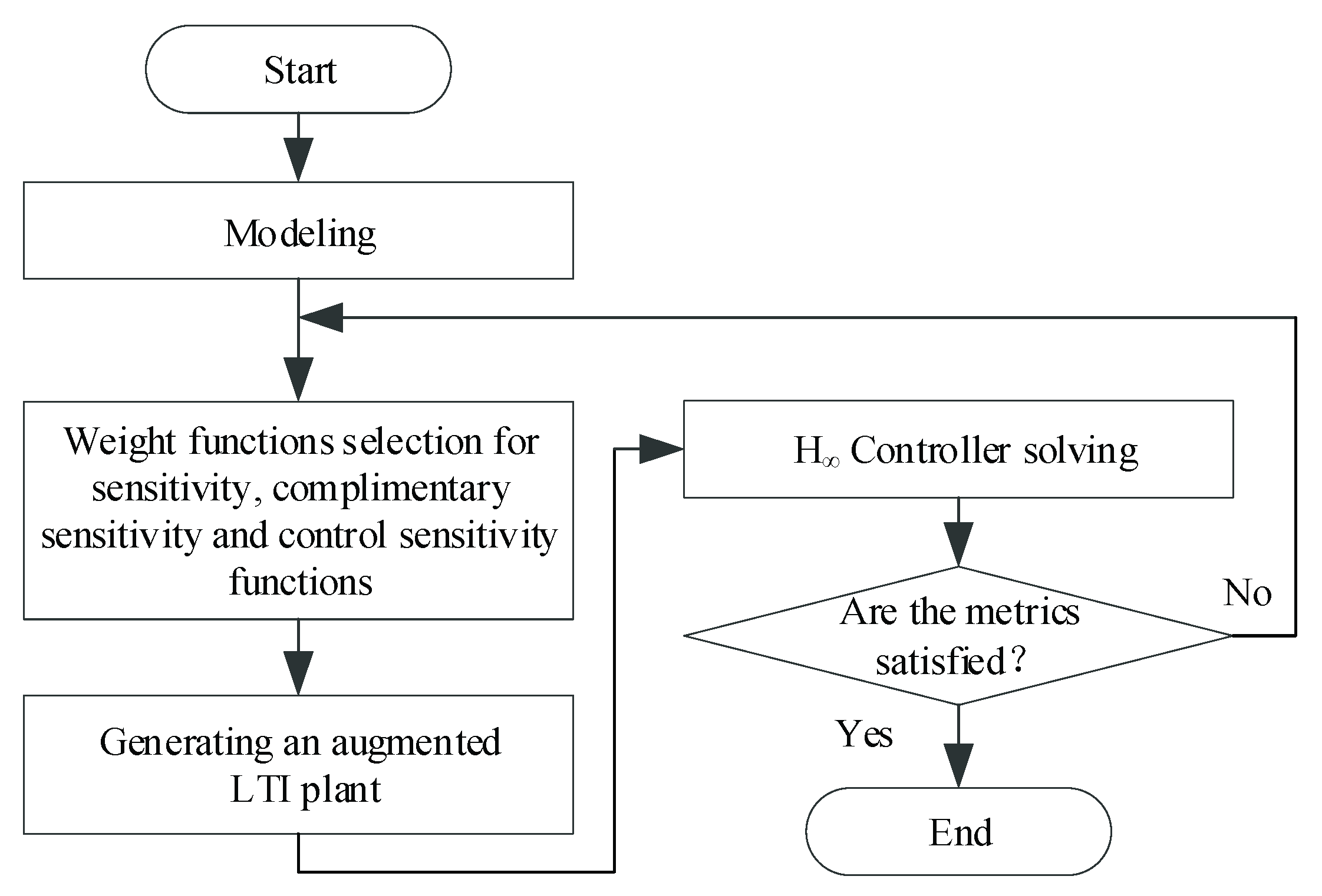
The general design procedure using H_∞ mixed sensitivity method is shown in Figure 7. The control plant modeling of TPC is derived in Section 2. Weight functions selection, which is an important step, will be discussed in this section. This selection has a significant influence on control performance and some instances is used to illustrate the design method. As shown in Figure 7, the step named “Generating an augmented LTI (linear time-invariant) plant” is used to create a state space model of augmented control plant with weight functions which is utilized for an H_∞ controller design (this task can be completed using the “augw” function in Matlab Robust Control Toolbox). The final step shown in Figure 5 is to solve the H_∞ controller using state space method [17]. Since the last two steps are relatively complex and mathematic, the details of the steps will not be discussed further in this section.

3.1. Fundamental of H_∞ Mixed Sensitivity Design

The standard model for H_∞ mixed sensitivity design is shown in Figure 8 [18]. W₁, W₂ and W₃ are weight function matrices, z₁, z₂ and z₃ are performance evaluation signal vectors, d is disturbance vector. r, e, u and y are reference vector, error vector, control signal vector and output vector respectively. K is the controller matrix and G is the control plant matrix.

The augmented control plant (20) can be obtained according to Figure 8.

$$\left[\begin{array}{c}{\mathit{z}}_1\\ {\mathit{z}}_2\\ {\mathit{z}}_3\\ \mathit{e}\end{array}\right]=\left[\begin{array}{c}{\mathit{W}}_1\mathit{e}\\ {\mathit{W}}_2\mathit{u}\\ {\mathit{W}}_3\mathit{y}\\ \mathit{e}\end{array}\right]=\left[\begin{array}{cc}{\mathit{W}}_1& -{\mathit{W}}_{\mathbf{1}}\mathit{G}\\ \mathbf{0}& {\mathit{W}}_2\\ \mathbf{0}& {\mathit{W}}_3\mathit{G}\\ \mathit{I}& -\mathit{G}\end{array}\right]\left[\begin{array}{c}\mathit{r}\\ \mathit{u}\end{array}\right]$$

(20)

Weight functions selection is the most important step in H_∞ mixed sensitivity design process, which will determine the control performance, such as disturbance attenuation, robustness and dynamic response ability.

A generalized closed loop transfer function matrix in (21) can be obtained by substituting u = Ke into (20)

$$\mathit{P}=\left[\begin{array}{c}{\mathit{W}}_1\mathit{S}\\ {\mathit{W}}_2\mathit{R}\\ {\mathit{W}}_3\mathit{T}\end{array}\right]$$

(21)

where ${\mathit{S}=(\mathit{I}+\mathit{G}\mathit{K})}^{-1}$ is called sensitivity function matrix, it is the transfer function matrix from d to e. ${\mathit{T}=\mathit{G}\mathit{K}(\mathit{I}+\mathit{G}\mathit{K})}^{-1}$ represents transfer function matrix from u to y. Since $\mathit{S}+\mathit{T}=\mathit{I}$, T is called complimentary sensitivity function matrix, ${\mathit{R}=\mathit{K}(\mathit{I}+\mathit{GK})}^{-1}$ is the transfer function matrix from e to u. In (21) W₁S is used to represents control performance requirements for disturbance rejection, and this performance metric can be designed by selecting appropriate W₁. The strength or the effectiveness of the control signal, u is restricted by W₂. W₃T represents requirements for robust stability, W₃ reflects the design constraints for multiplicative model uncertainty, it depends on the parameter deviations of control plants. In the frame of H_∞ mixed sensitivity control, the performance requirements for disturbance rejection and robust stability are interactive, however, performance balance (or tradeoff) can be obtained by proper weight functions design. Generally, the following factors should be considered in weight functions selection (scalars are used in following text for ease statement).

(1)

Considerations of W₁ Selection. W₁ represents the performance metric of the control system for disturbance rejection. For the sensitivity function matrix, S denotes the relationship between tracking error e and external disturbance d, while W₁ influences the tracking performance. It is desired that W₁ has a high gain in low frequency to reduce steady state error. And a steep declining slope of W₁ in high frequency is required for interference attenuation. Therefore, W₁ is usually selected as a high gain first order transfer function. Furthermore, the crossover frequency, f_w1 of W₁ should be lower than the desired crossover frequency of the corrected control subsystem.

(2)

Considerations of W₂ Selection. The strength or effectiveness of control signal u in Figure 8 can be limited by W₂, which is beneficial for keeping u in its allowable range, therefore controller saturation and overshooting can be effectively avoided. The amplitude of u will be reduced if the gain of W₂ is increased. The gain of W₂ can be rationally high according to the required control performance. The bandwidth of control system can be influenced by W₂, the control bandwidth will be reduced if the gain of W₂ is increased and vice versa. Therefore, W₂ should be appropriately designed by taking into account the effectiveness of the control signal and control bandwidth requirement. In order to avoid high order of the resulted controller, W₂ is often selected as a constant in practices.

(3)

Considerations of W₃ Selection. W₃ is selected as a metric for multiplicative perturbation. Generally, the nominal transfer function can used to represent the characteristics of control plant accurately in low frequency, while the accuracy will be degraded in high frequency range, deviations in gain and phase will be resulted accordingly. This type of deviation can be expressed as multiplicative uncertainty, which is usually used to describe parameter uncertainty and high frequency unmodeled dynamic of the system. Multiplicative uncertainty, Δ(s) can be obtained by solving (22).

$$\Delta (s)=\frac{G_{\Delta }(s)-G_0(s)}{G_0(s)}=\frac{G_{\Delta }(s)}{G_0(s)}-1$$

(22)

In (22), G₀ and G_Δ are nominal transfer function and practice transfer function, respectively.

In a mixed sensitivity design method, the gain W₃ should be designed to guarantee that Δ(s) in (22) is properly covered by W₃ (as shown in Figure 9 and Figure 10). W₃ always has a high pass characteristic to make sure that the corrected control system has a favorable performance to attenuate high frequency disturbance. And the crossover frequency W₃, f_w3 should be higher than the desired crossover frequency of the corrected control subsystem. Taking into account the crossover frequency of W₁, the crossover frequency of the corrected control subsystem will be located between f_w1 and f_w3. More systematic and detailed discussions about weight functions selection can be found in references [19,20].

3.2. H_∞ Controller Design

For (18) and (19), the values of G₁₁ and G₂₂ will be changed with the variation of steady state operation point, the load change can be represented by different values of R_L, and there are deviations between the nominal values of C_d1, C_d2, L_d1, r_e and their corresponding actual values. By using (22), the model deviation caused by the mentioned factors can be described through multiplicative uncertainty.

According to the parameters listed in

Table 1. Simulation Parameters.

Parameter/Unit.	Value
vd1/V	24
vd2/V	50
vd3/V	36
Turns ratio N1:N2:N3	1:1:1
L1/μH	55
L2/μH	55
L3/μH	55
Ld1/μH	100
RL/Ω	90/30
Cd1/μF	1200
Cd2/μF	1000
Switching frequency/kHz	20

, assuming C_d2 has ± 25 % deviation from its nominal value. The equation in (23) can be selected as W₃₁.

$$W_{31}=2.0250\times {10}^{-4}s+0.75$$

(23)

The possible multiplicative uncertainties of G_ov (denoted by dashed lines) and the Bode plot (solid line) of W₃₁ are shown in Figure 9. It can be seen that the crossover frequency of W₃₁ is about 520 Hz. Similarly, ±25 % parameter deviation for C_d1 and L_d1 are assumed respectively, W₃₂ shown in (24) is selected to cover the multiplicative uncertainty of G_oc.

$$W_{32}=2.34\times {10}^{-6}{s}^2+0.00156s+0.26$$

(24)

The Bode plots of W₃₂ (solid line) and multiplicative uncertainties (dashed lines) with different parameter values are shown in Figure 10. The crossover frequency of W₃₂ in this case is about 90 Hz.

The weight functions, W₁₁ and W₁₂ shown in (25) are designed for the sensitivity functions of current and voltage subsystem respectively, the crossover frequencies of W₁₁ and W₁₂ are 127 Hz and 26 Hz, respectively.

$${\mathit{W}}_1=\left[\begin{array}{cc}{W}_{11}& 0\\ 0& W_{12}\end{array}\right]=\left[\begin{array}{cc}\frac{800}{s+0.001}& 0\\ 0& \frac{800}{5s+0.001}\end{array}\right]$$

(25)

The weight functions, W₂₁ and W₂₂ given in (26) are used to restrict the control signals.

$${\mathit{W}}_2=\left[\begin{array}{cc}{W}_{21}& 0\\ 0& W_{22}\end{array}\right]=\left[\begin{array}{cc}0.1& 0\\ 0& 0.9\end{array}\right]$$

(26)

According to the parameters listed in Table 1, the resulted robust controllers for current and voltage control subsystems are obtained in (27) and (28) respectively (the controller can be solved using “hinfsyn” function in Matlab Robust Control Toolbox).

$$G_{\mathrm{c}}=\frac{4234s+7.057\times {10}^4}{s^2+6043s+6.043}$$

(27)

$$G_{\mathrm{v}}=\frac{5777s^2+5.777\times {10}^{5}s+4.814\times {10}^{10}}{s^3+1.367\times {10}^5{s}^2+1.376\times {10}^{8}s+2.751\times {10}^4}$$

(28)

The Bode plot of the corrected voltage control subsystem is shown in Figure 11, the crossover frequency is about 243 Hz and the phase margin is about 76°. The Bode plot of the corrected current control subsystem is presented in Figure 12, the crossover frequency of the current control loop is about 59 Hz, the gain margin is about 51 dB and the phase margin is about 70°. It can be seen from Figure 12 that there is a notch in the Bode plot of the resulted H_∞ controller by which the resonant peak of the uncorrected system can be cancelled accordingly, therefore, a smooth Bode plot of the corrected system is obtained.

As shown in (19), G_oc will manifest a weak damping characteristic if r_e is very small and there is a significant resonant peak in the Bode plot of G_oc. If G_v and G_c are designed as a proportional-integral (PI) controller, and the crossover frequency of the corrected current loop by PI controller is expected to be lower than the resonant frequency (about 460 Hz) of G_oc, in this condition, in order to avoid 0 dB axis intersecting with the corrected current control around the resonant frequency of G_oc, the crossover frequency should be greatly reduced. As seen in Figure 13, $G_{\mathrm{c}}=0.0144+36/\mathrm{s}$ is utilized, the crossover frequency of the corrected current control system is about f_c = 7 Hz, the gain margin is about 9dB and the phase margin is about 89°. For comparison, if a higher crossover frequency of the corrected current control subsystem is wanted with a PI controller, for example, with about f_c = 60 Hz (like that in Figure 12 using H_∞ control method) with $G_{\mathrm{c}}=0.17+425/s$, as presented by the dashed line shown in Figure 13, the resulted current control subsystem will be unstable under this condition, because the Bode plot of the corrected current control system crosses 0 dB axis twice around its resonant peak. In contrast, since the resulted current controller, G_c designed by H_∞ mixed sensitivity method in Figure 12 has a natural notch at the resonant frequency of G_oc, which can cancel the negative impact of G_oc resonance effectively, the improved current control performance can be obtained accordingly.

4. Simulation and Experimental

4.1. Simulation Results

A simulation model of the proposed design method is developed in MATLAB/Simulink environment to verify the effectiveness of the proposed method. The parameters used in the simulation model are presented in Table 1. The simulation results for changing the current reference, $i_{\mathrm{ds}}^{*}$ with different control methods are presented in Figure 14. The simulation results using a PI controller are shown in Figure 14a. In this figure, the current reference value is reduced from 2.1 A to 1 A (at 0.25 s) and then suddenly increased again to 2.1 A (at 0.4 s). It can be seen the actual current, i_ds can track its reference signal. However, since the current control bandwidth is relatively low in this condition, it takes about 30 ms to reach the reference current value. And the output voltage, v_d2 is almost kept constant in this process. With the same reference change condition, the simulation results using H_∞ controller are shown in Figure 14b, as it can be concluded from this figure that the dynamic response speed of i_ds is much faster than that in Figure 14a, the transient state process time is decreased to about 7 ms. And it can be seen in Figure 14 that the battery current i_d3 is increased from about −0.22 A to about 0.5 A and then to −0.22 A with the corresponding change of $i_{\mathrm{ds}}^{*}$, the dynamic response speed with H_∞ controller in Figure 14b is much faster than that with a PI controller in Figure 14a.

Figure 15 shows the simulation results of a sudden load change test. In Figure 15a, the load resistor value is reduced from 60 Ω to 30 Ω (the load is increased from about 42 W to about 83 W) at 0.25 s and then suddenly increased to 60 Ω at 0.4 s again. In the transient state process, due to the interaction of voltage and current control subsystems, there are fluctuations in i_ds and v_d2 simultaneously at the load change moment. With the same load change condition, the simulation results with H_∞ robust controller are given in Figure 15b. Though the fluctuations in v_d2 and i_d3 are similar to that in Figure 15a, the amplitudes of fluctuations and the transient recovery time of i_ds in Figure 15b are significantly reduced compared to that in Figure 15a.

4.2. Experiment Results

An experimental hardware shown in Figure 16 is developed to validate the theoretical design and simulation results. The parameter deviations of C_d1 (about 1130 μF), L_d1 (about 107 μH) and C_d2 (about 1046 μF) are limited to 10% of their nominal value (this condition can be easily guaranteed in practice). The other parameters used in the experimental tests are approximately identical to the simulation parameters listed in Table 1. The experiment results are presented in Figure 17, Figure 18, Figure 19, Figure 20, Figure 21 and Figure 22.

Figure 17 shows the experiment results of v_d2 and i_ds using the PI controller. The current reference value is changed from 1 A to 2.1 A and reduced to 1 A again suddenly in Figure 17a,b respectively, and the corresponding transient state process times are about 32 ms and 31 ms. Under the same reference value change condition, the experiment results using H_∞ controller are shown in Figure 18. Since the current control bandwidth using H_∞ controller (59 Hz) is higher than that using a PI controller (7 Hz), the transient state process times shown in Figure 18a,b are 19 ms and 23 ms respectively, which are much shorter than that in Figure 17.

With the same reference value change condition being used in Figure 17, the corresponding experiment results of battery current, i_d3 using PI and H_∞ controllers are shown in Figure 19 and Figure 20, respectively. It can be seen that the changes of battery current are much faster in Figure 20 than that in Figure 19. Compared to Figure 19a, less time is taken in Figure 20a for the battery current to reach its steady state value due to a higher control bandwidth of the H_∞ controller. A similar result can also be obtained by comparing Figure 19b with Figure 20b.

The load change experiment results using PI and H_∞ controllers are shown in Figure 21 and Figure 22 respectively. In Figure 21a, the load resistor is changed from 90 Ω to 30 Ω (the load is increased from about 28 W to about 83 W) instantaneously, which causes about a 0.5 V voltage drop in v_d2 (the peak value of ∆v_d2) and about a 280 mA current drop in i_ds. In Figure 22a, the corresponding voltage and current drops are 140 mA and 0.5 V respectively with the same load change. When the load resistor is again increased from 30 Ω to 90 Ω (the load is decreased from about 83 W to 28 W), a 200 mA current increment is produced in i_ds using a PI controller in Figure 21b, and an 80 mA current increment is caused in i_ds using an H_∞ controller in Figure 22b. It can be concluded that the interaction between voltage control subsystem and current control subsystem is better attenuated by adopting an H_∞ controller. Furthermore, the voltage fluctuation is reduced from 0.5 V in Figure 21b to about 0.38 V in Figure 22b with the H_∞ controller when the load resistor is increased.

In contrast to the traditional PI controller, the experiment results indicate that the negative impact caused by the couplings between current control subsystem and voltage control subsystem can be effectively suppressed by using the H_∞ controller. And the dynamic response performance of the control system can also be improved with the proposed method.

5. Conclusions

An H_∞ mixed sensitivity method is introduced in this paper for three-port converter control. The H_∞ mixed sensitivity method has an inherent characteristic to balance performance and stability of a control system through the use of an appropriate weight functions selection. The H_∞ current controller manifests a superior characteristic of effectively damping the resonant peak of the current control subsystem that can reduce limitations in the control bandwidth design, and this is beneficial for enhancing the stability of the current control subsystem. The simulation and experiment results show that the resulted optimal H_∞ controller has advantages in dynamic response performance and load disturbance rejection compared to a traditional proportional-integral (PI) controller.

References

1. Tao, H.; Kotsopoulos, A.; Duarte, J.L.; Hendrix, M.A.M. Family of multiport bidirectional DC-DC converters. IEE Proc. Electr. Power Appl. 2006, 153, 451–458. [Google Scholar] [CrossRef]
2. Vázquez, N.; Sánchez, C.M.; Hernández, C.; Vázquez, E.; Lesso, R. A three port converter for renewable energy applications. In Proceedings of the IEEE International Symposium on Industrial Electronics, Gdansk, Poland, 27–30 June 2011; pp. 1736–1740. [Google Scholar]
3. Wu, H.; Sun, K.; Ding, S.; Xing, Y. Topology derivation of non-isolated three-port DC-DC converters from DIC and DOC. IEEE Trans. Power Electron. 2013, 28, 3297–3307. [Google Scholar] [CrossRef]
4. Zhu, H.; Zhang, D.; Zhang, B.; Zhou, Z. A non-isolated three-port DC-DC converter and three-domain control method for PV-battery power systems. IEEE Trans. Ind. Electron. 2015, 62, 4937–4947. [Google Scholar] [CrossRef]
5. Phattanasak, M.; Ghoachani, R.G.; Martin, J.P.; Mobarakeh, B.N.; Pierfederici, S.; Davat, B. Control of a hybrid energy source comprising a fuel cell and two storage devices using isolated three-port bidirectional DC-DC converters. IEEE Trans. Power Electron. 2015, 51, 491–497. [Google Scholar] [CrossRef]
6. Liu, R.; Xu, L.; Kang, Y.; Hui, Y.; Li, Y. Decoupled TAB Converter with Energy Storage System for HVDC Power System of More Electric Aircraft. J. Eng. 2018, 2018, 593–602. [Google Scholar] [CrossRef]
7. Jakka, V.N.S.R.; Shukla, A.; Demetriades, G.D. Dual-Transformer-Based Asymmetrical Triple-Port Active Bridge (DT-ATAB) Isolated DC–DC Converter. IEEE Trans. Ind. Electron. 2017, 64, 4549–4560. [Google Scholar] [CrossRef]
8. Zhao, C.; Kolar, J.W. A novel three-phase three-port UPS employing a single high-frequency isolation transformer. In Proceedings of the 2004 IEEE 35th Annual Power Electronics Specialists Conference, Aachen, Germany, 20–25 June 2004. [Google Scholar]
9. Zhao, C.; Round, S.D.; Kolar, J.W. An Isolated Three-Port Bidirectional DC-DC Converter with Decoupled Power Flow Management. IEEE Trans. Power Electron. 2008, 23, 2443–2453. [Google Scholar] [CrossRef]
10. Tao, H.; Kotsopoulos, A.; Duarte, J.L.; Hendrix, M.A.M. Transformer-Coupled Multiport ZVS Bidirectional DC–DC Converter with Wide Input Range. IEEE Trans. Power Electron. 2008, 23, 771–781. [Google Scholar] [CrossRef]
11. Wang, L.; Wang, Z.; Li, H. Asymmetrical Duty Cycle Control and Decoupled Power Flow Design of a Three-port Bidirectional DC-DC Converter for Fuel Cell Vehicle Application. IEEE Trans. Power Electron. 2012, 27, 891–904. [Google Scholar] [CrossRef]
12. Falcones, S.; Ayyanar, R. LQR control of a quad-active-bridge converter for renewable integration. In Proceedings of the 2016 IEEE Ecuador Technical Chapters Meeting (ETCM), Guayaquil, Ecuador, 12–14 October 2016. [Google Scholar]
13. Tao, H.; Kotsopoulos, A.; Duarte, J.L.; Hendrix, M.A.M. A soft-switched three-port bidirectional converter for fuel cell and supercapacitor applications. In Proceedings of the IEEE 36th Power Electronics Specialists Conference, Recife, Brazil, 12–16 June 2005; pp. 2487–2493. [Google Scholar]
14. Falcones, S.; Ayyanar, R.; Mao, X. A DC–DC multiport-converter-based solid-state transformer integrating distributed generation and storage. IEEE Trans. Power Electron. 2013, 28, 2192–2203. [Google Scholar] [CrossRef]
15. Zhang, J.; Wu, H.; Cao, F.; Zhu, L.; Xing, Y. Modeling and Decoupling Control of Three-port Half-bridge Converters. Proc. CSEE 2015, 35, 671–678. [Google Scholar]
16. You, J.; Liao, M.; Chen, H.; Ghasemi, N.; Vilathgamuwa, M. Disturbance Rejection Control Method for Isolated Three-Port Converter with Virtual Damping. Energies 2018, 11, 3204. [Google Scholar] [CrossRef]
17. Doyle, J.C.; Glover, K.; Khargonekar, P.P.; Francis, B.A. State-space solutions to standard H2 and H control problems. IEEE Trans. Autom. Control 1989, 34, 831–847. [Google Scholar] [CrossRef]
18. Zhou, K.; Doyle, J.C.; Glover, K. Robust and Optimal Control; Prentice Hall: Upper Saddle River, NJ, USA, 1996. [Google Scholar]
19. Wu, X.; Xie, X. Weight Function Matrix Selection in H Robust Control. J. Tsinghua Univ. 1997, 37, 27–30. [Google Scholar]
20. Hu, J.; Unbehauen, H.; Bohn, C. A practical approach to selecting weighting functions for H control and its application to a pilot plant. In Proceedings of the UKACC International Conference on Control ’96, Exeter, UK, 2–5 September 1996; pp. 998–1003. [Google Scholar]
Figure 1. Conventional structure of a DC microgrid.
Energies 12 02231 g001
Figure 2. Multiport DC/DC converter based structure of a DC microgrid.
Energies 12 02231 g002
Figure 3. Topology, equivalent circuit and modulation scheme of isolated three-port converter (a) topology of the isolated three-port converter, (b) equivalent Δ-connection circuit, (c) modulation scheme.
Energies 12 02231 g003
Figure 4. Equivalent circuit model of a dual active bridge.
Energies 12 02231 g004
Figure 5. Decoupled model.
Energies 12 02231 g005
Figure 6. Control diagram block of the TPC system.
Energies 12 02231 g006
Figure 7. Design procedure of H mixed sensitivity based controller.
Energies 12 02231 g007
Figure 8. H mixed sensitivity standard design model.
Energies 12 02231 g008
Figure 9. Bode plots of W31 and multiplicative uncertainty of Gov.
Energies 12 02231 g009
Figure 10. Bode plots of W32 and multiplicative uncertainty of Goc.
Energies 12 02231 g010
Figure 11. Bode of voltage control loop with H robust controller.
Energies 12 02231 g011
Figure 12. Bode of current control loop with H robust controller.
Energies 12 02231 g012
Figure 13. Bode of current control loop with a PI controller.
Energies 12 02231 g013
Figure 14. Simulation results with current reference change using a (a) PI controller, (b) H controller.
Energies 12 02231 g014
Figure 15. Simulation results with load change using a (a) PI controller, (b) H controller.
Energies 12 02231 g015
Figure 16. Hardware experiment circuit of three-port converter.
Energies 12 02231 g016
Figure 17. vd2 and ids using a PI controller with i ds * is (a) increased, (b) decreased.
Energies 12 02231 g017
Figure 18. vd2 and ids using H controller with i ds * is (a) increased, (b) decreased.
Energies 12 02231 g018
Figure 19. vd2 and id3 using a PI controller with i ds * is (a) increased, (b) decreased.
Energies 12 02231 g019
Figure 20. vd2 and id3 using H controller with i ds * is (a) increased, (b) decreased.
Energies 12 02231 g020
Figure 21. vd2, ids and Δvd2 using a PI controller with RL is (a) decreased, (b) increased.
Energies 12 02231 g021
Figure 22. vd2, ids and Δvd2 using H controller with RL is (a) decreased, (b) increased.
Energies 12 02231 g022