Robust Localization for Robot and IoT Using RSSI


Abstract
1. Introduction
2. Ranging with RSSI Method
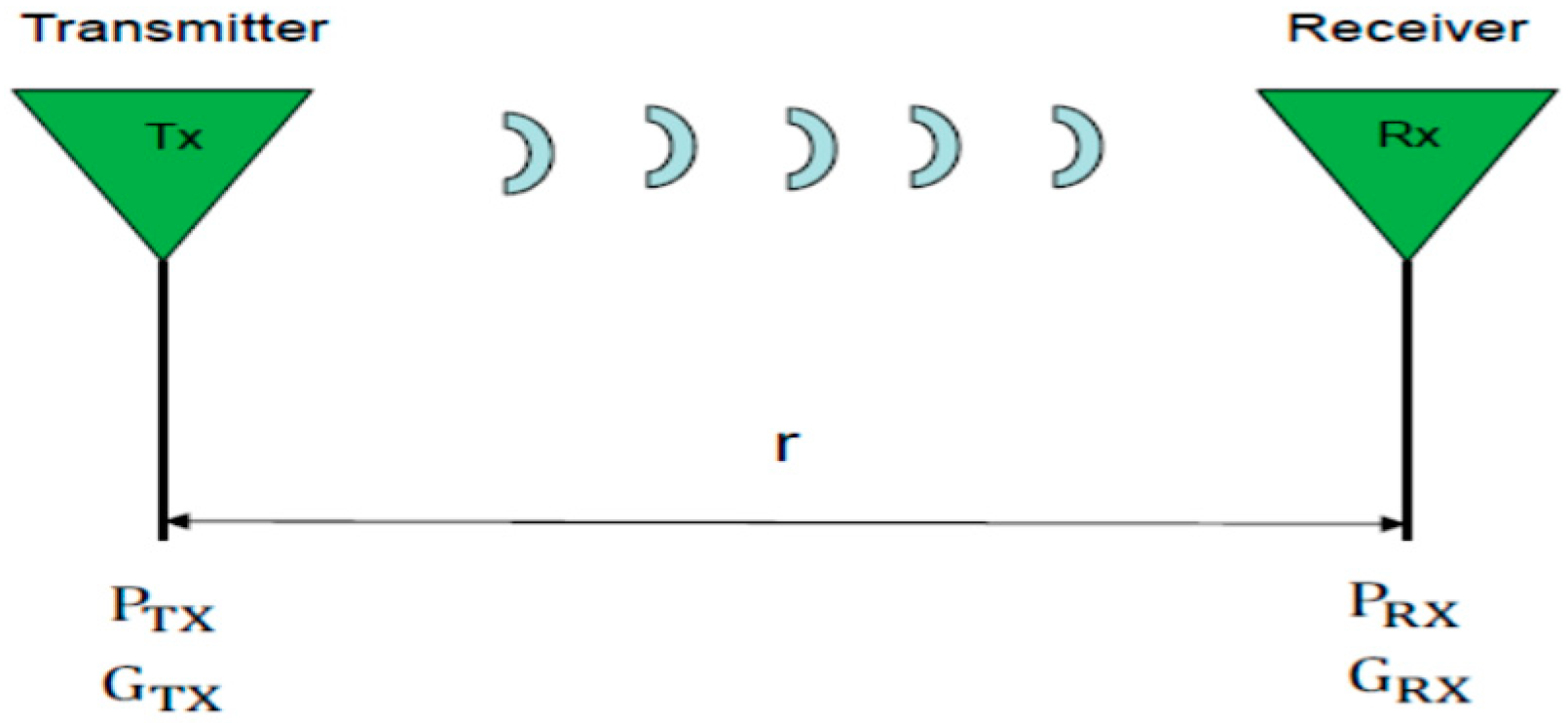
2.1. Signal-Propagation Model
2.2. Power Law Model
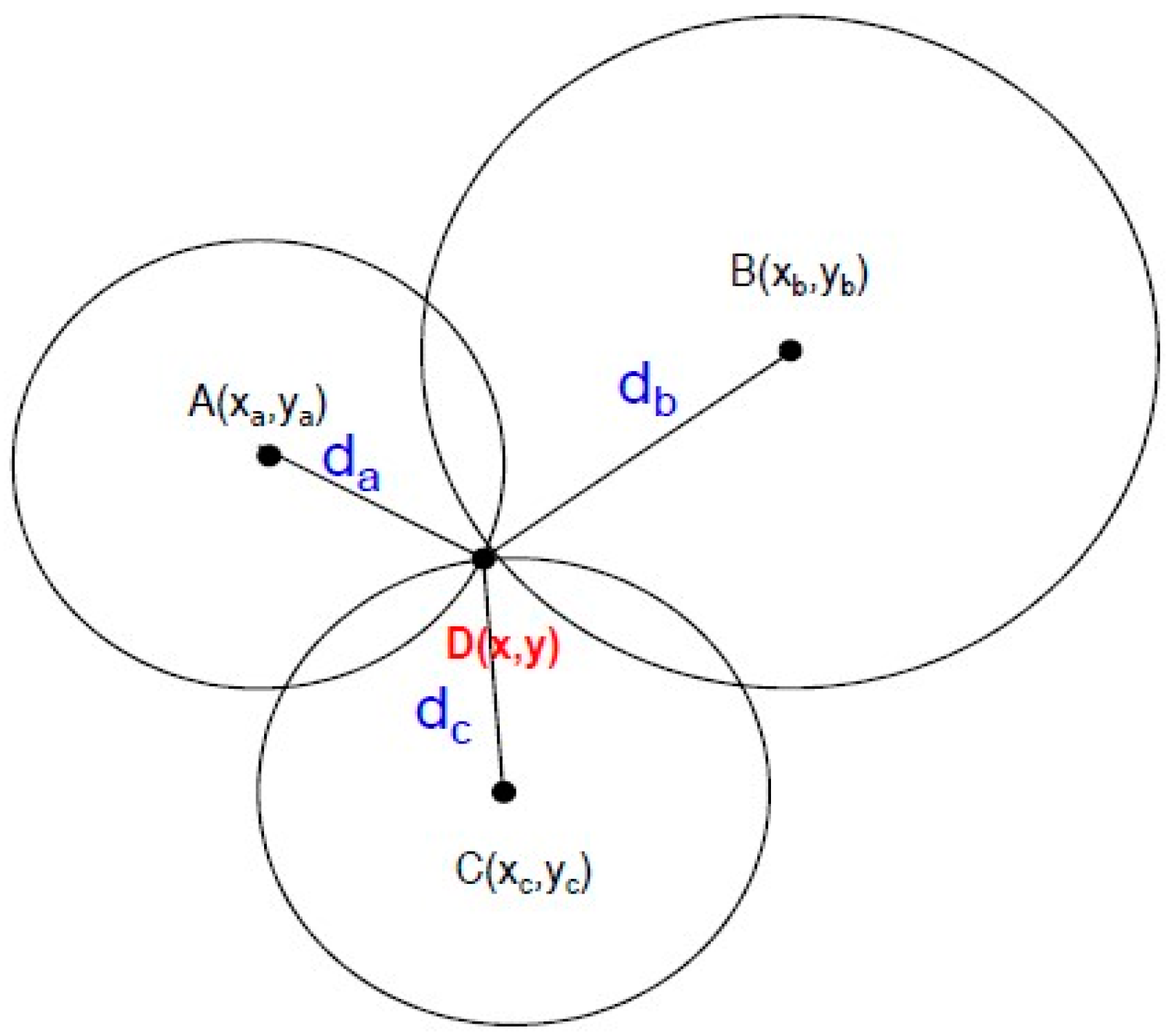
2.3. Position Estimation with Trilateral Technique
3. Simulation Using RSSI with the Trilateral Technique
3.1. RSSI Algorithm
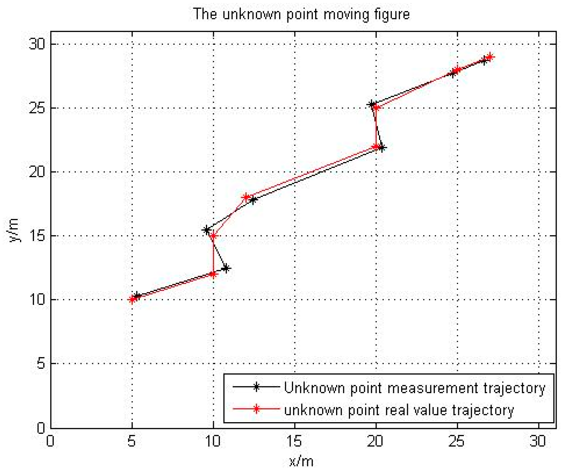
3.2. Computer Simulation
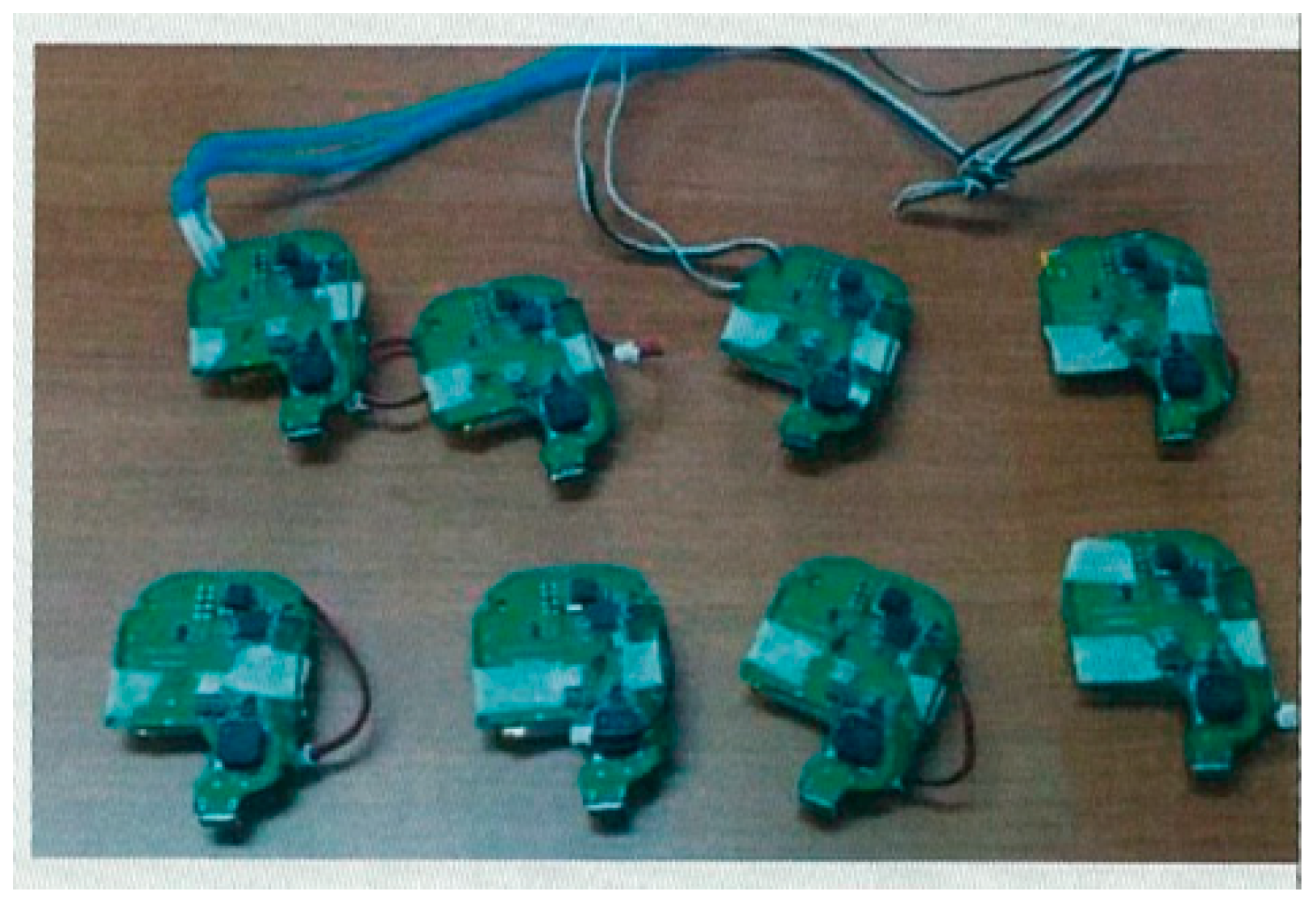
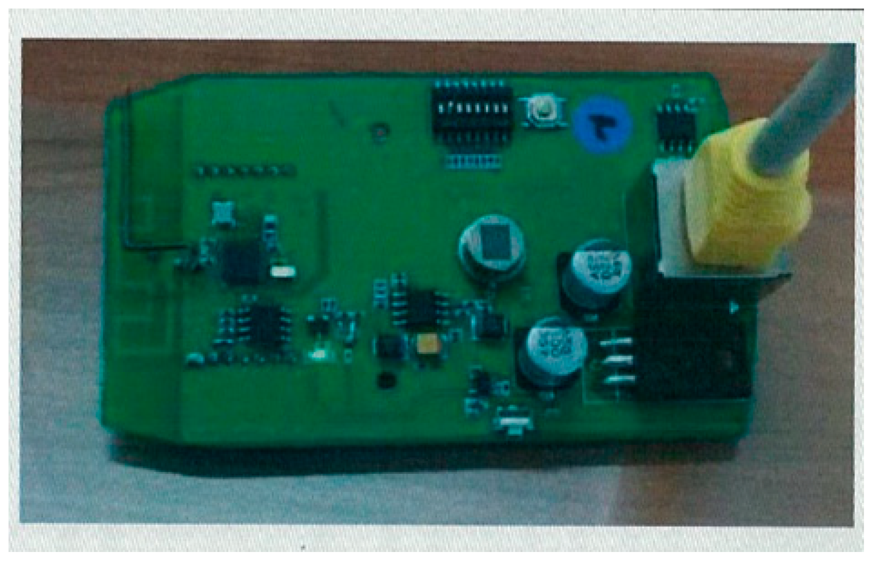
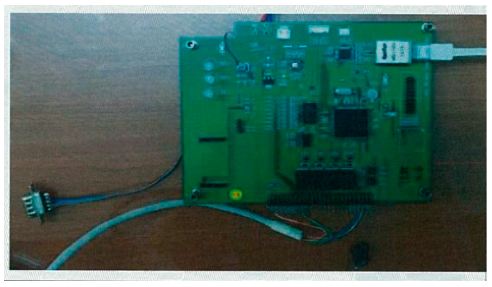
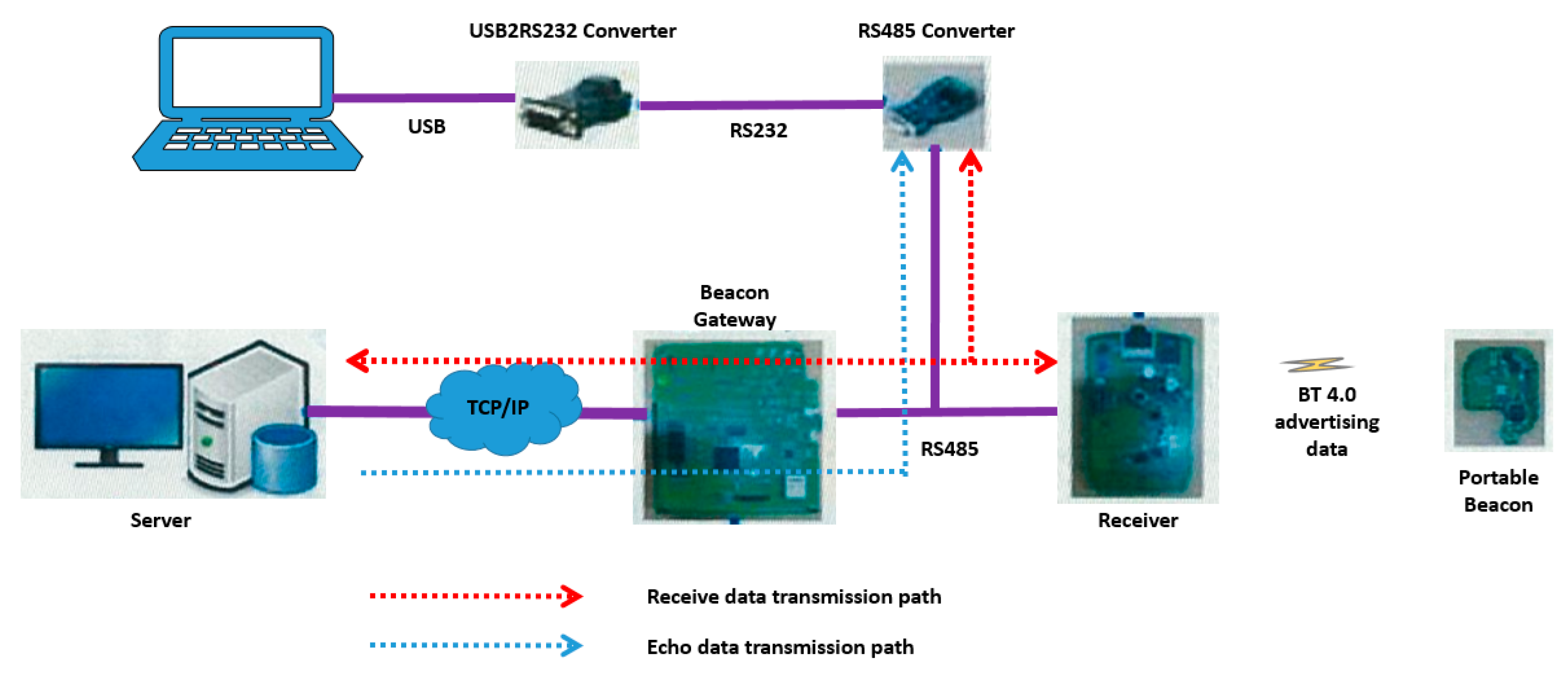
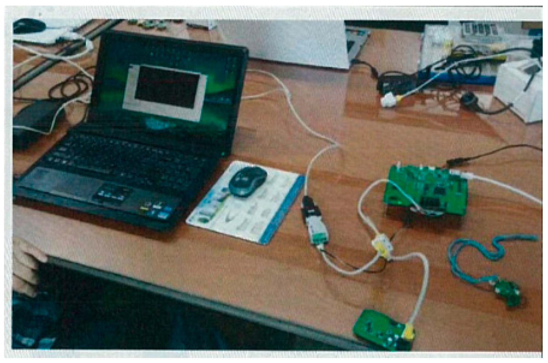
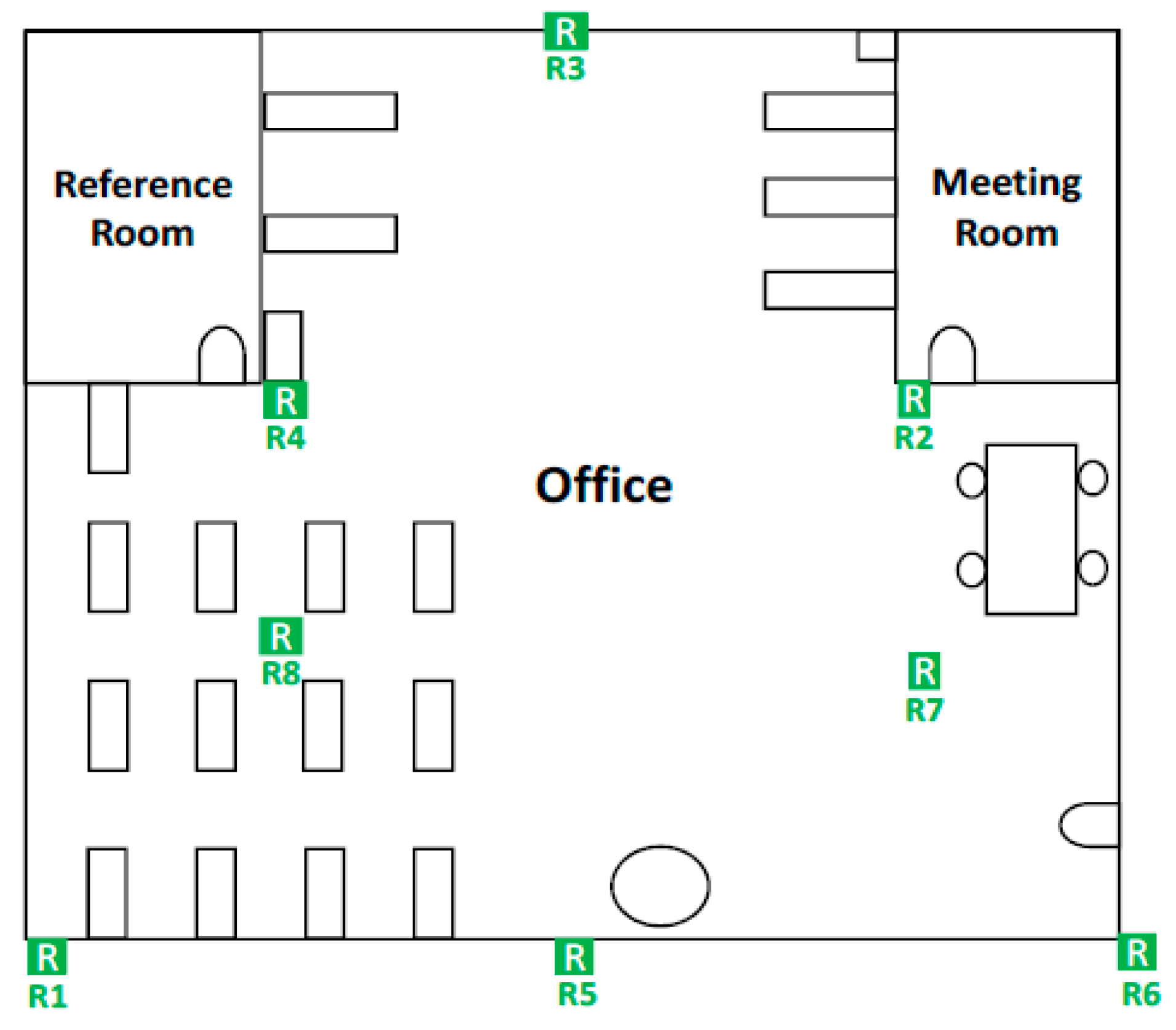
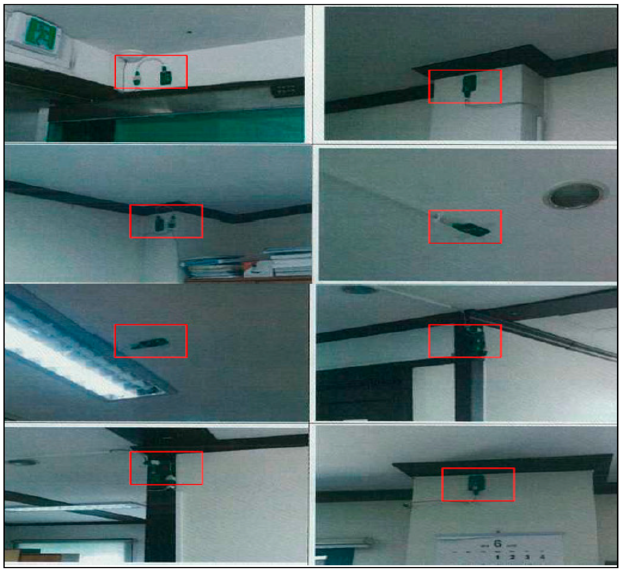
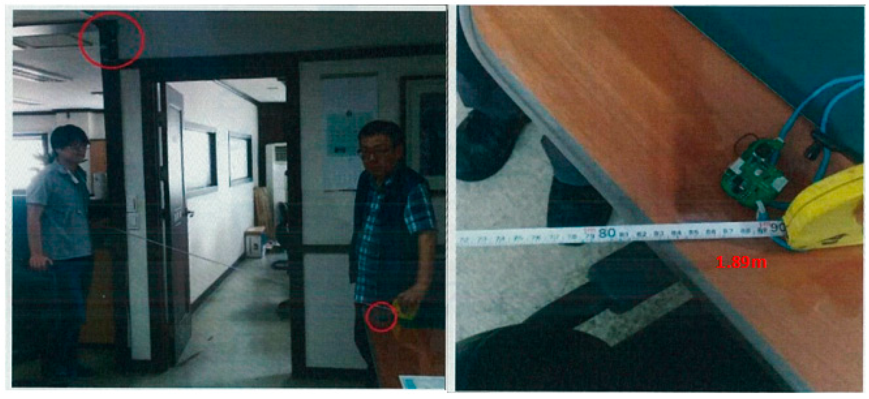
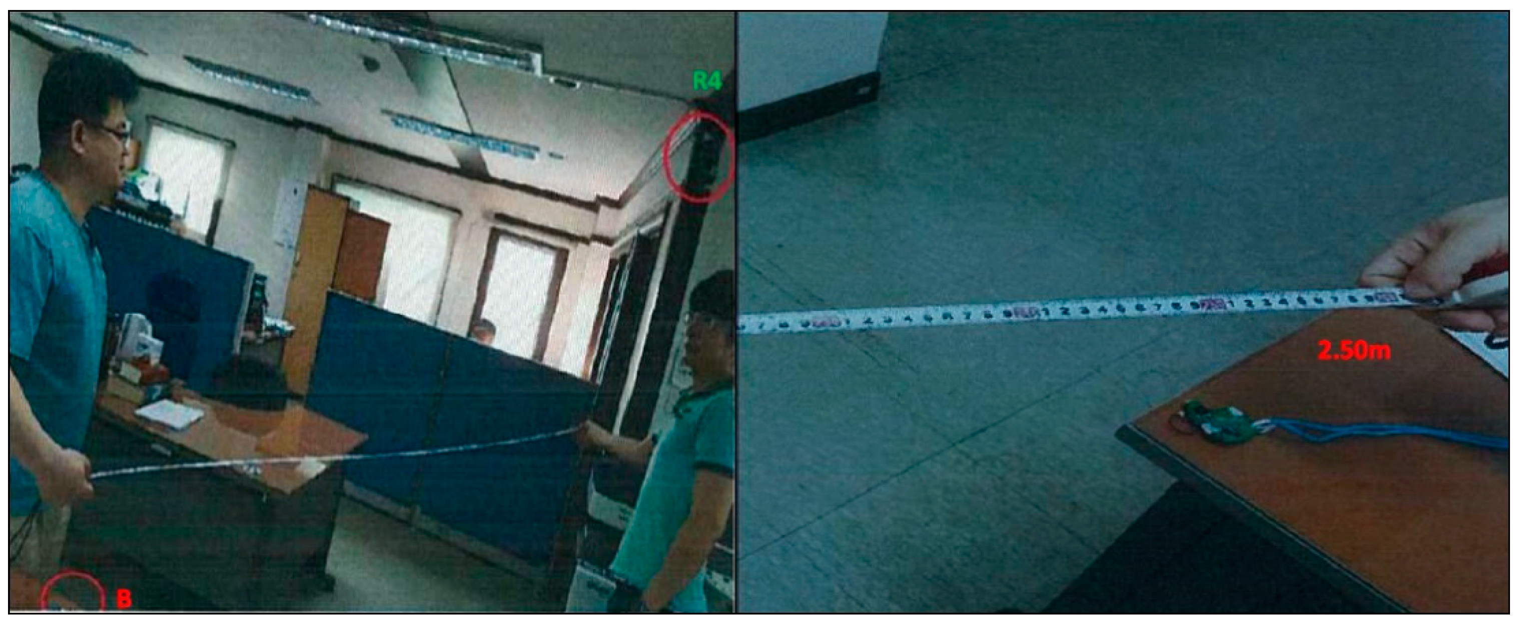
4. Experimental Device and Result
4.1. Case 1
4.2. Case 2
5. Conclusion
Funding
Conflicts of Interest
References
- Gao, J.; Gao, X.; Zhu, W.; Zhu, J.; Wei, B. Mobile robot room location system design and research. Inf. Comput. Autom. 2008, 3, 923–926. [Google Scholar]
- Mohareri, O.; Rad, A.B. Vision-based location positioning system VIA augmented reality: An application in humanoid robot navigation. Inter. J. Humanoid Robo. 2013, 10, 1350019. [Google Scholar] [CrossRef]
- Liu, Y.; Yang, J.; Wu, Z. Ubiquitous and cooperation network robot system within a service framework. Inter. J. Humanoid Robo. 2011, 8, 147–167. [Google Scholar] [CrossRef]
- Yang, T.H.; Yi, S.; Qi, D.; Tao, H.; Xu, C.R. The Locating method by measuring its acceleration for in-pipelines inspection robots. Inf. Comput. Autom. 2008, 3, 931–934. [Google Scholar]
- Shon, Y. Scientometric, Analysis for the IOT of service oriented and next generation smart device. J. Kor. Inst. Elect. Comm. Sci. 2015, 10, 721–728. [Google Scholar] [CrossRef]
- Hu, L.; Jiang, J.; Zhou, J. Environment observation system based on semantics in the internet of things. J. Networks 2013, 8, 2721–2727. [Google Scholar] [CrossRef]
- Karl, H.; Willing, A. Protocols and Architectures for Wireless Sensor Networks; John Wiley & Sons, Inc.: Hoboken, NJ, USA, 2005. [Google Scholar]
- Akyildiz, I.F. Wireless sensor networks: A survey. Comput. Networks 2002, 38, 393–422. [Google Scholar] [CrossRef]
- Wang, C.; Xiao, L. Sensor localization under limited measurement capabilities. IEEE Network 2007, 21, 16–23. [Google Scholar] [CrossRef]
- Sairah, N.; Ko, N.Y. Analysis of indoor robot localization using ultrasonic sensors. Int. J. Fuzzy Logic Intell. Syst. 2014, 14, 41–48. [Google Scholar]
- Gabriel, H.; Fay, H.; Reinhard, K. Landmark initialization for unscented Kalman filter sensor fusion in monocular camera localization. Int. J. Fuzzy Logic Intell. Syst. 2013, 13, 1–10. [Google Scholar]
- Mao, G.; Fidan, B.; Brian, D.; Anderson, O. Wireless sensor network localization techniques. Comput. Networks 2007, 51, 2529–2553. [Google Scholar] [CrossRef]
- Bram, D.; Stefan, D.; Havinga, P. Wireless Sensor Networks: Range-based Localization in Mobile Sensor Networks; EWSN: Zurich, Switzerland, 2006; pp. 164–179. [Google Scholar]
- Mazur, V.; Williams, E.; Boldi, R.; Maier, L.; Proctor, D.E. Initial comparison of lightning mapping with operational time-of-arrival and interferometric systems. J. Geophys. Res. D 1997, 102, 11071–11085. [Google Scholar] [CrossRef]
- Pulgarín, J.; Younes, C.; del Río, D. Electromagnetic fields generated by lightning channels with tortuosity and its effect on the time-of-arrival technique. In Proceedings of the 12th International Symposium on Lightning Protection, Belo Horizonte, Brazil, 7–11 October 2013; pp. 140–144. [Google Scholar]
- Salimi, B.; Abdul-Malek, Z.; Mehranzamir, K.; Mashak, S.V.; Afrouzi, H.N. Localized single-station lightning detection by using TOA method. J. Teknologi 2013, 64, 73–77. [Google Scholar]
- Bekcibasi, U.; Tenruh, M. Increasing RSSI localization accuracy with distance reference anchor in wireless sensor networks. Acta Polytech. Hungarica 2014, 11, 103–120. [Google Scholar]
- Alippi, C.; Vanini, G. A RSSI-based and calibrated centralized localization technique for wireless sensor networks. In Proceedings of the Fourth Annual IEEE International Conference on Pervasive Computing and Communications Workshops, Pisa, Italy, 13–17 March 2006; pp. 301–306. [Google Scholar]
- Pradhan, S.; Bae, Y.; Pyun, J.Y.; Ko, N.Y.; Hwang, S.S. Hybrid TOA Trilateration Algorithm Based on Line Intersection and Comparison Approach of Intersection Distances. Energies 2019, 12, 1668. [Google Scholar] [CrossRef]
- Wang, J.; Urriza, P.; Han, Y.; Cabric, D. Weighted Centroid Localization Algorithm: Theoretical Analysis and Distributed Implementation. IEEE Trans. Wirel. Commun. 2011, 10, 3403–3413. [Google Scholar] [CrossRef]
- Roberts, R. TDOA localization techniques, working group for wireless personal area networks (WPANs). 2004. Available online: https://www.enriquedans.com/wp-content/uploads/2013/03/TDOA-localization-techniques.pdf (accessed on 7 June 2019).
- Kułakowski, P.; Vales-Alonso, J.; Egea Lopez, E.; Ludwin, W.; García-Haro, J. Angle-of-arrival localization based on antenna arrays for wireless sensor networks. Comput. Electri. Eng. 2010, 36, 1181–1186. [Google Scholar] [CrossRef]
- Scherhaufl, M.; Pichler, M.; Ziroff, A.; Stelzer, A. Phase-of-arrival-based localization of passive UHF RFID tags. In Proceedings of the IEEE MTT-S International Microwave Symposium Digest (MTT), Seattle, WA, USA, 2–7 June 2013; pp. 1–3. [Google Scholar]
- Han, G.; Xu, H.H.; Duong, T.Q.; Jiang, J.F.; Hara, T. Localization algorithms of Wireless Sensor Networks: A survey. Telecommun. Syst. 2013, 52, 2419–2436. [Google Scholar] [CrossRef]
- He, T.; Huang, C.; Blum, B.-M.; Stankovic, J.A.; Abdelzaher, T. Range-free localization schemes for large scale sensor networks. In Proceedings of the 9th annual international conference on Mobile computing and networking, San Diego, CA, USA, 14–19 September 2003; pp. 81–95. [Google Scholar]
- Paraxnvir, B.; Venkata, P.N. RADAR: An inbuilding RF-based user location and tracking system. In Proceedings of the IEEE INFOCOM, Tel Aviv, Israel, 26–30 March 2000; pp. 775–784. [Google Scholar]
- Thomas, F.; Ros, L. Revisiting trilateration for robot localization. IEEE Trans. Rob. 2005, 21, 93–101. [Google Scholar] [CrossRef]
- Lau, E.-E.-L.; Chung, W.Y. Enhanced RSSI-Based Real-Time User Location Tracking System for Indoor and Outdoor Environments. In Proceedings of the International Conference on Convergence Information Technology, Gyeongju, South Korea, 21–23 November 2007; pp. 1213–1218. [Google Scholar]
- Shuo, S.; Hao, S.; Yang, S. Design of an experimental indoor position system based on RSSI. In Proceedings of the 2nd International Conference on Information Science and Engineering, Hangzhou, China, 4–6 December 2010; pp. 1989–1992. [Google Scholar]
- Peng, W.W.; Xin, W. Research on robot indoor localization method based on wireless sensor network. In Proceedings of the International Conference on Advances in Mechanical Engineering and Industrial Informatics, Zhengzhou, China, 11–12 April 2015; pp. 1025–1040. [Google Scholar]
- Ning, G.; Gang, W.Z.; Gang, S.K. Research on Indoor Positioning Algorithm Based on Trilateral Positioning and Taylor Series Expansion. In Proceedings of the International Conference on Computational Modeling, Simulation and Applied Mathematics, Bangkok, Thailand, 24–25 July 2016. [Google Scholar]
- Friis, H.T. A note on a simple transmission formula. Proc. IRE. 1946, 34, 254–256. [Google Scholar] [CrossRef]


| Algorithm | Error (m) | 6 times RMS (m) | 100 times RMS | ||||
|---|---|---|---|---|---|---|---|
| 1 | 2 | 3 | 4 | 5 | |||
| Weighted Centroid-locating algorithm [22] | 4.4283 | 4.1263 | 2.2145 | 7.5029 | 6.985 | 5.40 | 5.29 |
| RSSI locating algorithm [20] | 2.3065 | 1.7712 | 4.1526 | 3.1047 | 1.1119 | 2.70 | 1.97 |
| TOA-locating algorithm [19] | 0.2154 | 0.1130 | 0.2444 | 1.1266 | 0.1121 | 0.17 | 0.12 |
| Number | RSSI A (dBm) | RSSI B (dBm) | RSSI C (dBm) | RMS Error (m) |
|---|---|---|---|---|
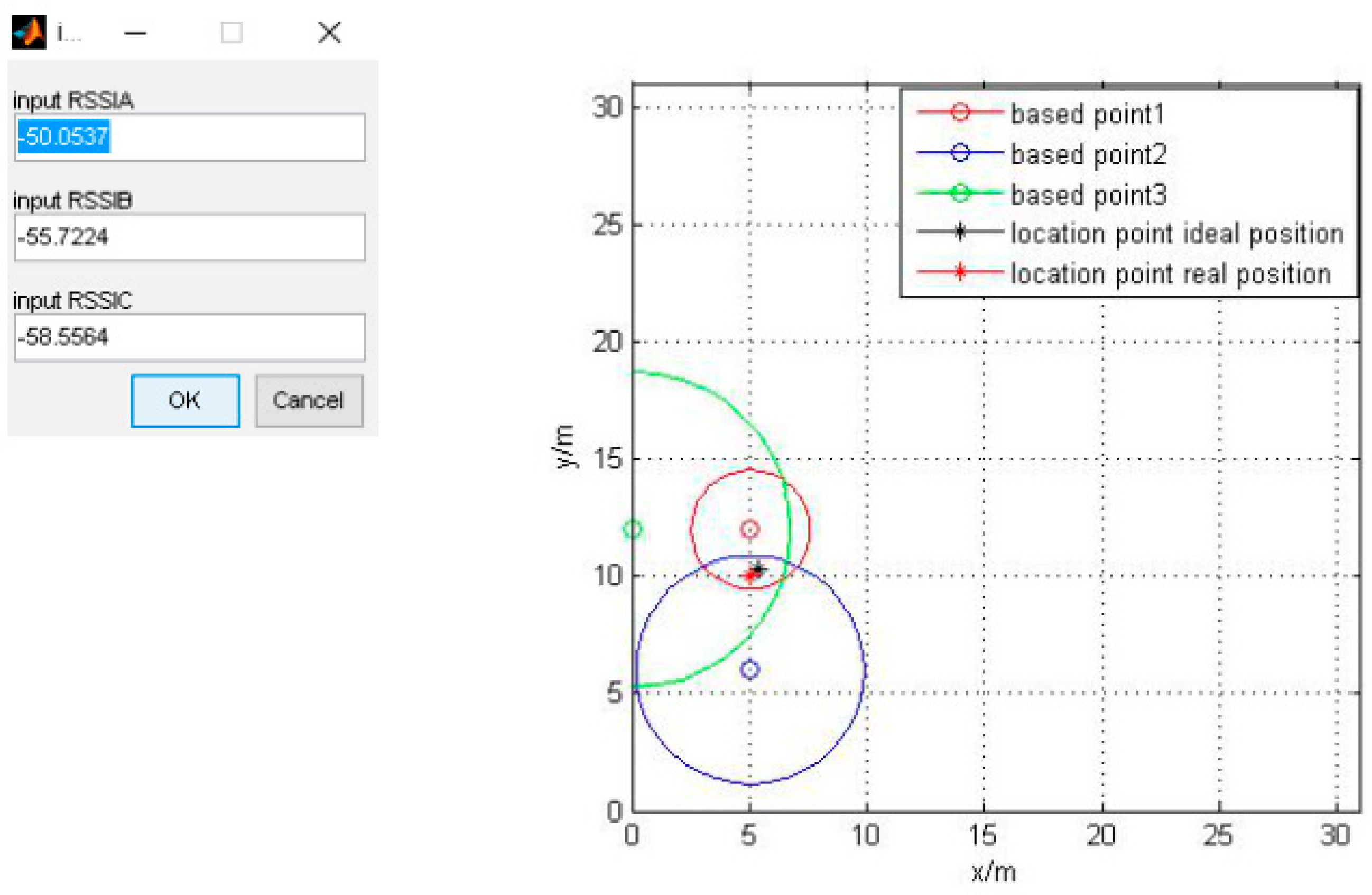
| Figure 5 | −50.0537 | −55.7224 | −58.5564 | 0.536 |
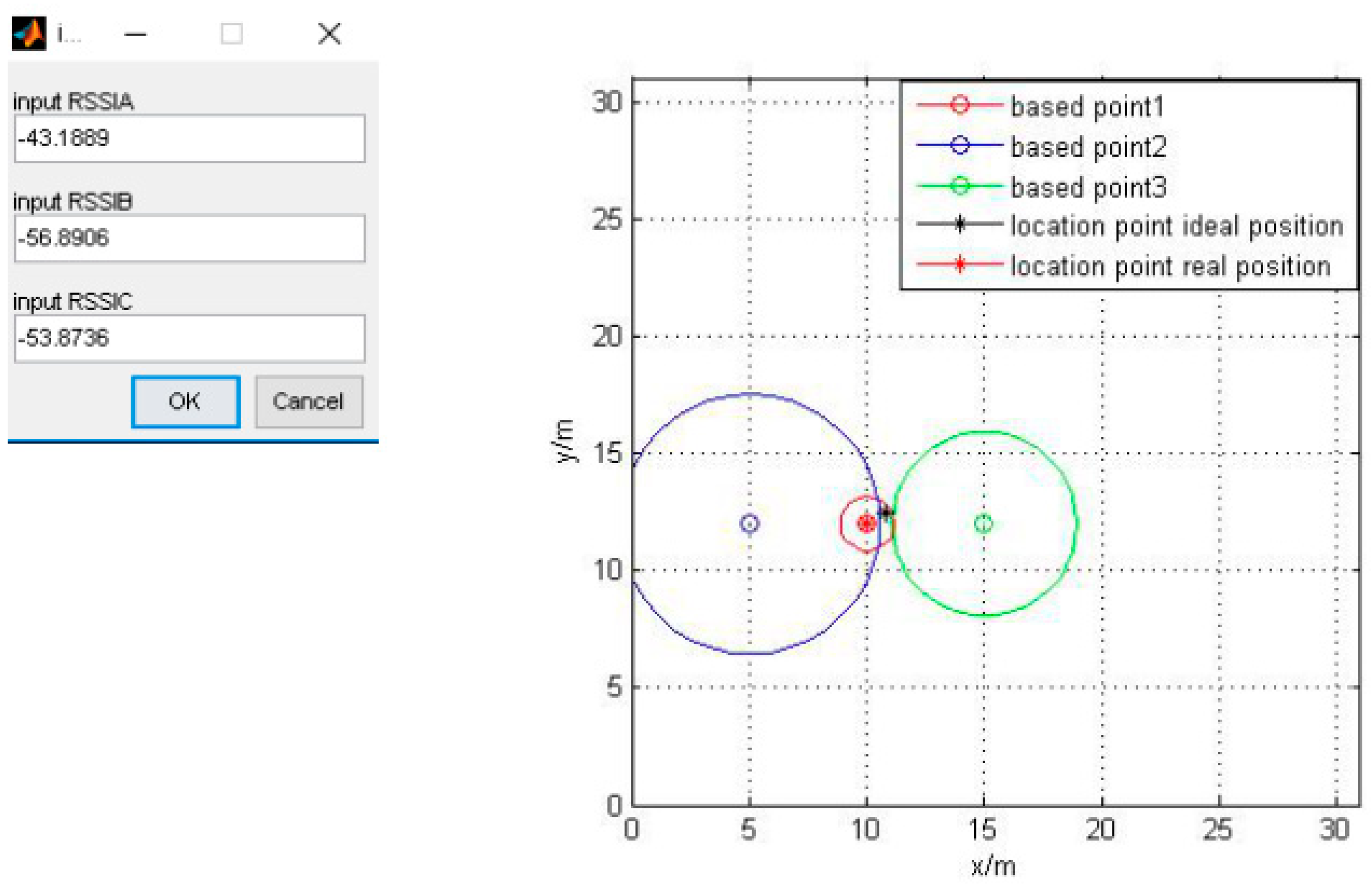
| Figure 6 | −43.1889 | −56.8906 | −53.8736 | |
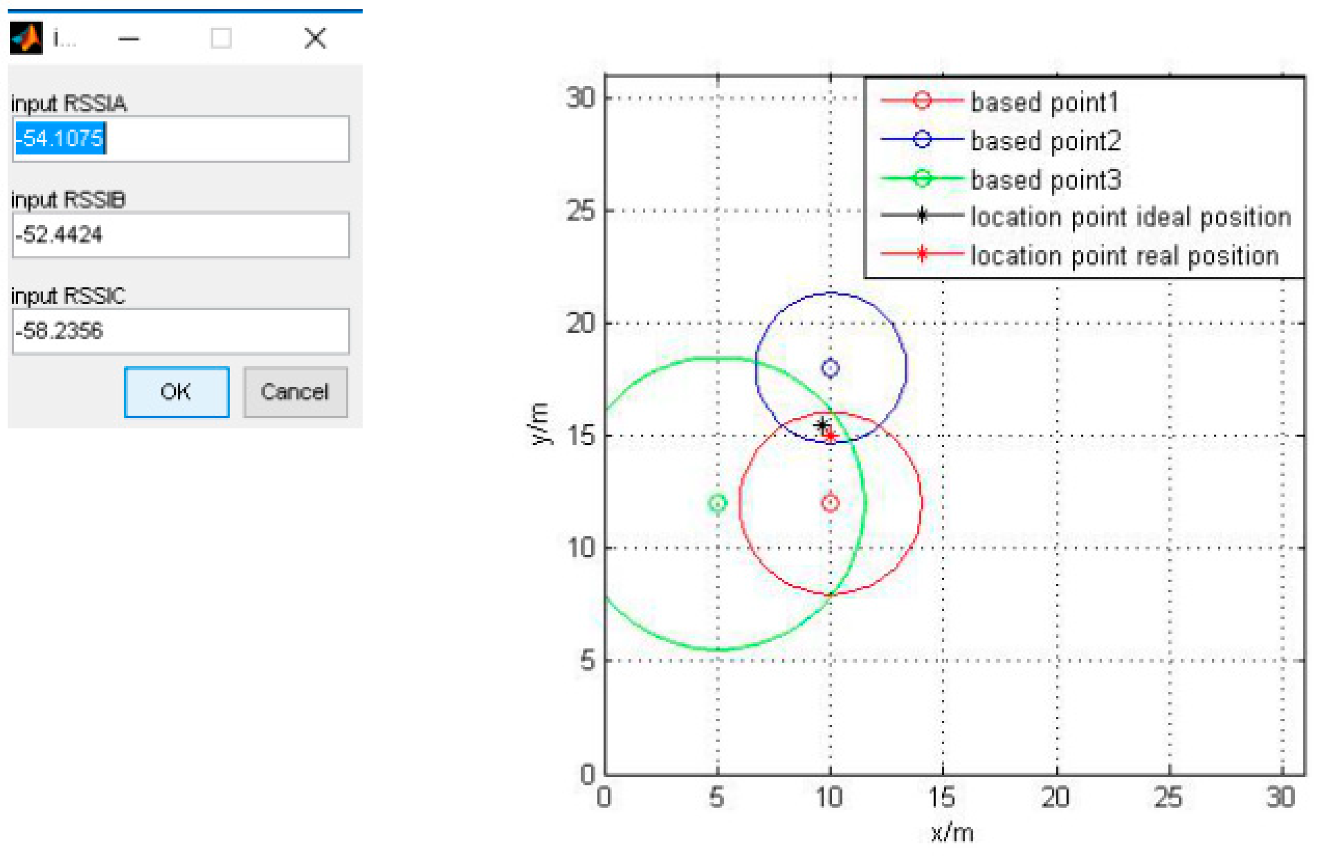
| Figure 7 | −54.1075 | −52.4424 | −58.2356 | |
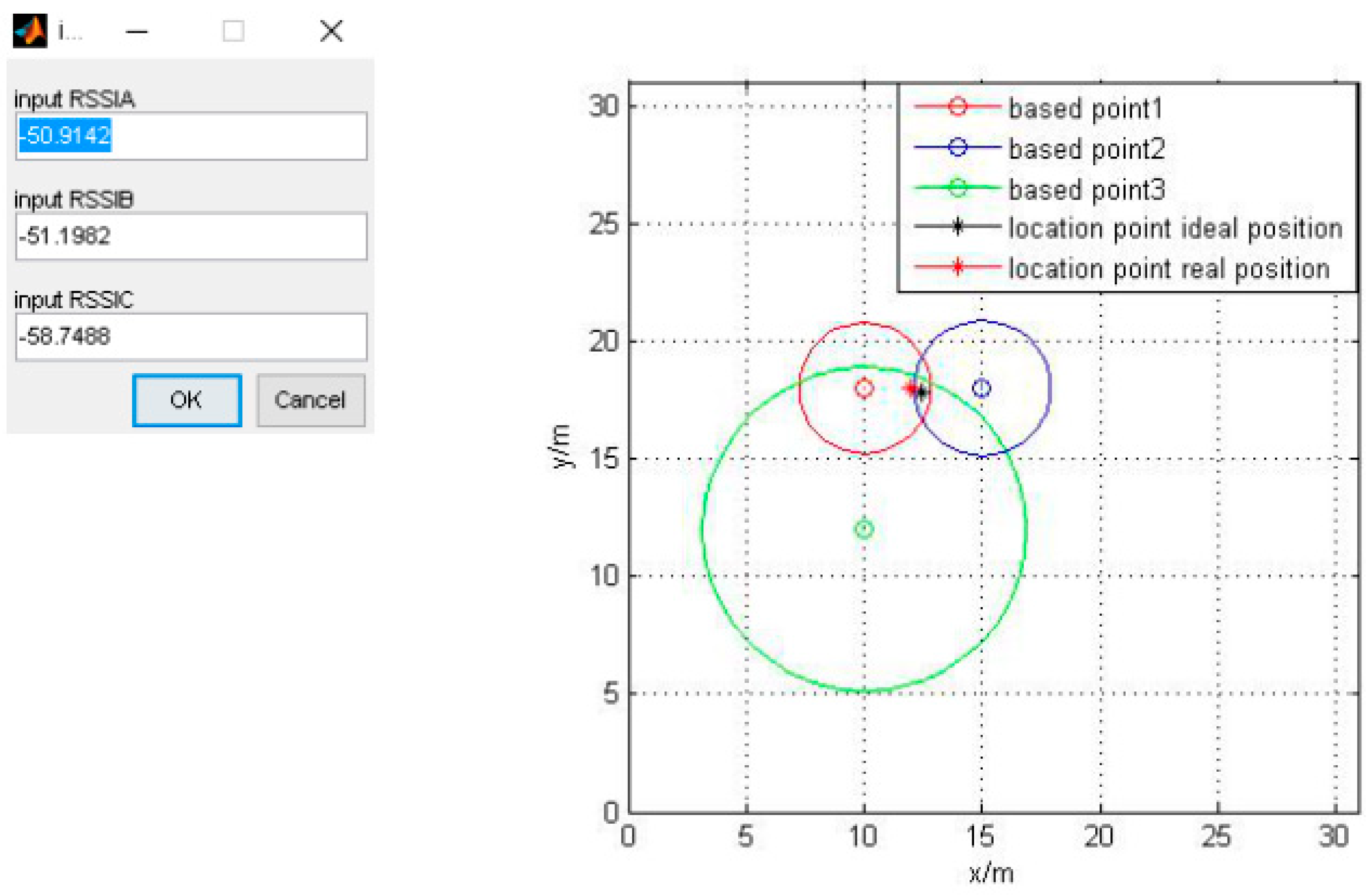
| Figure 8 | −50.9142 | −51.1982 | −58.7488 | |
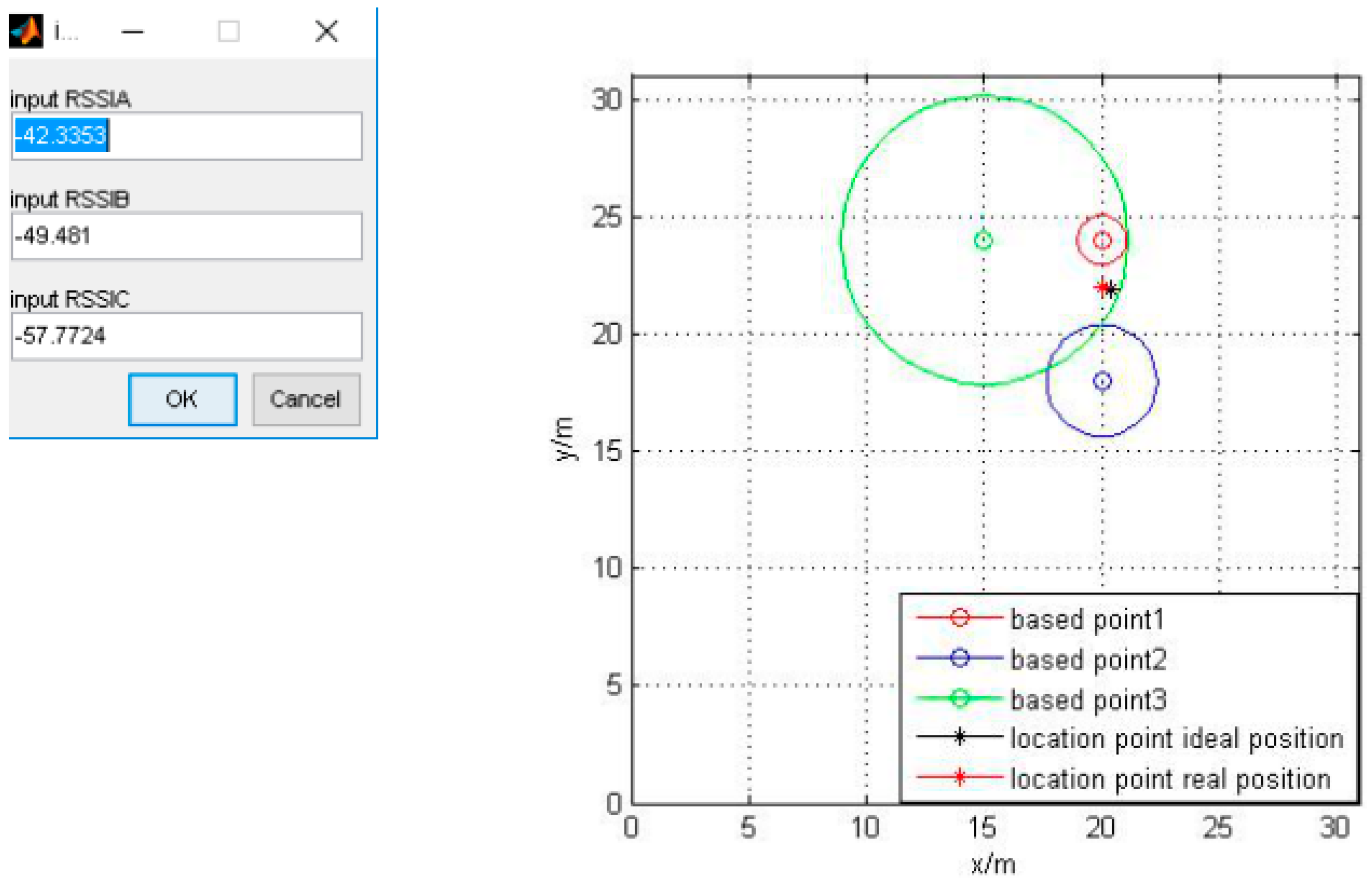
| Figure 9 | −42.3353 | −49.481 | −57.7724 | |
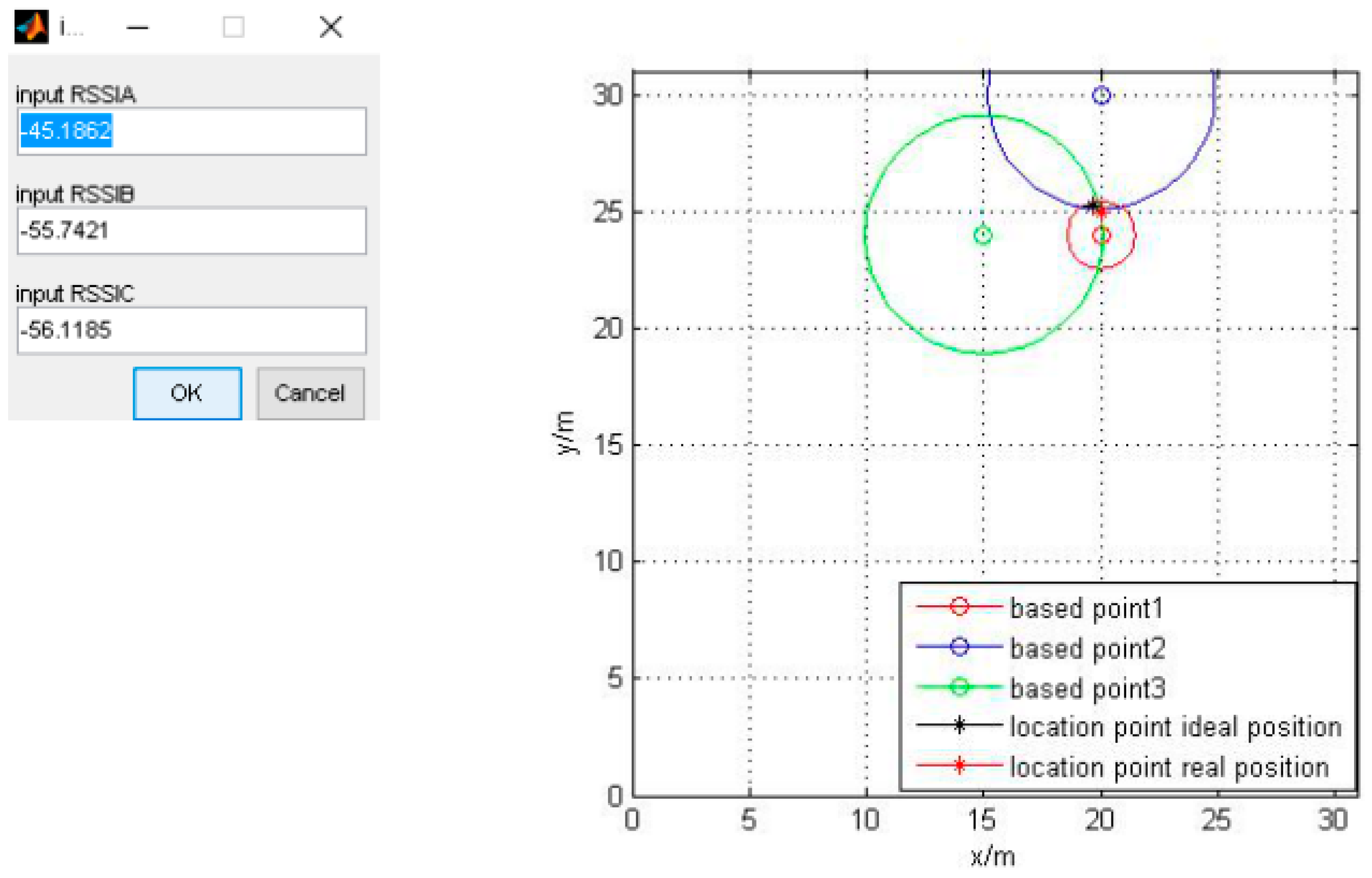
| Figure 10 | −45.1862 | −55.7421 | −56.1185 | |
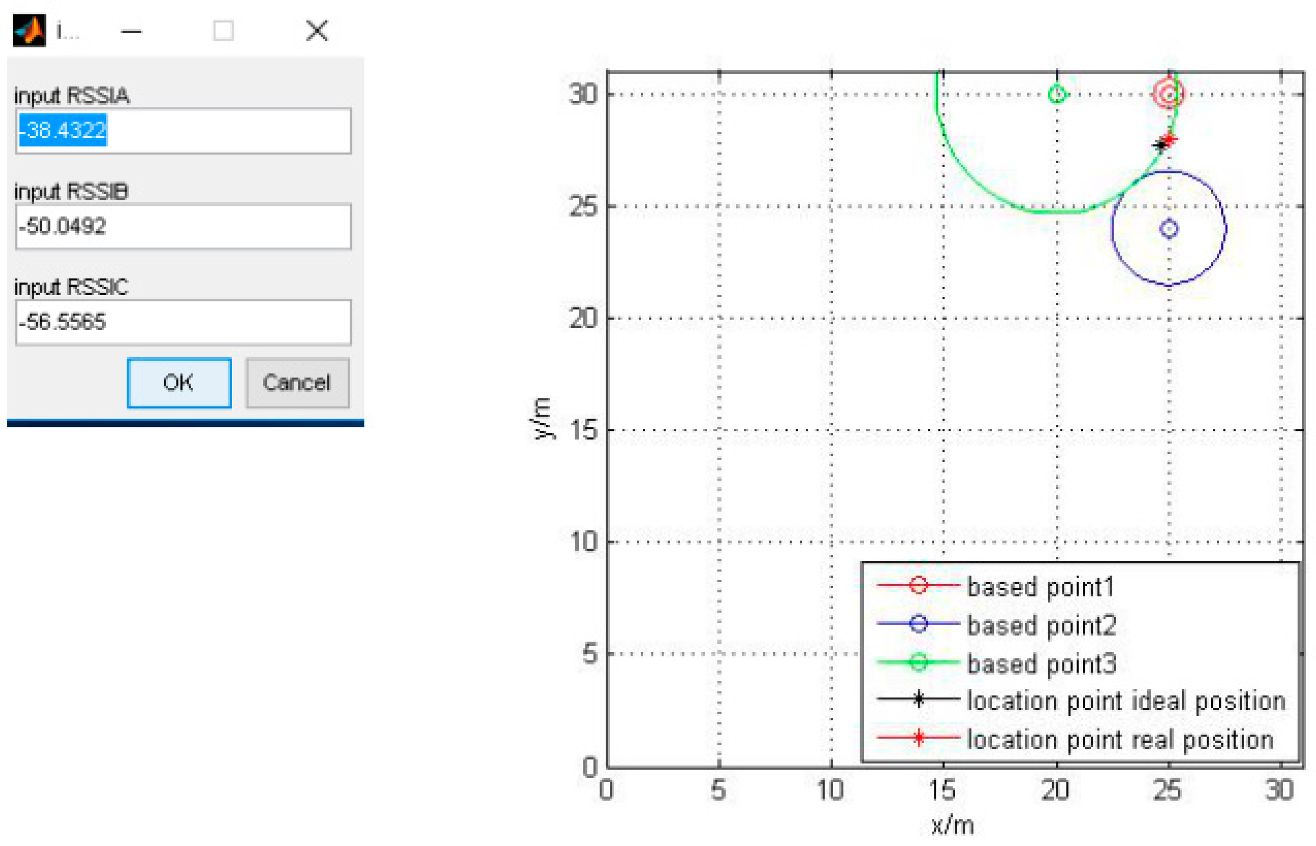
| Figure 11 | −38.4322 | −50.0492 | −56.5565 | |
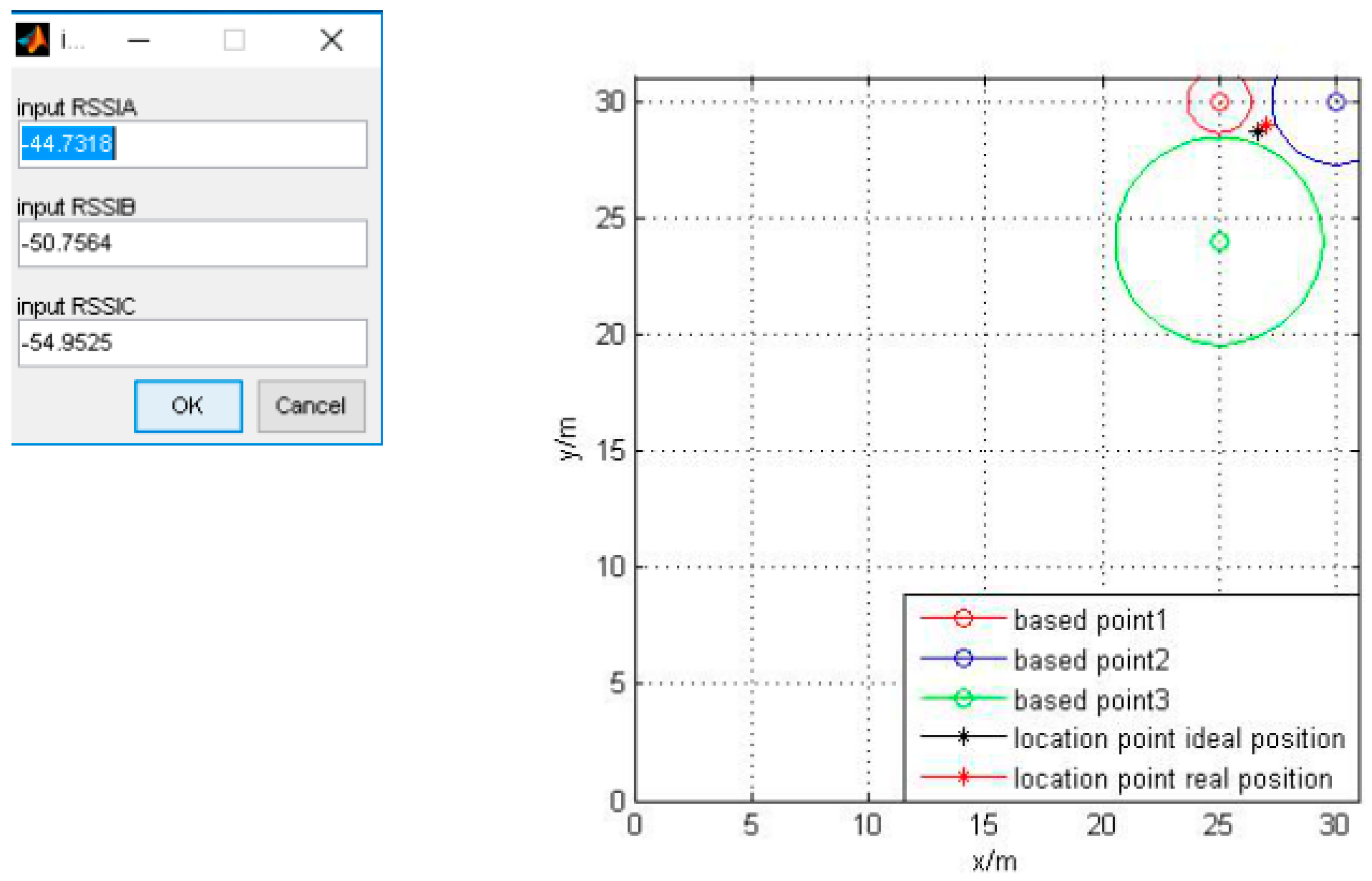
| Figure 12 | −44.7318 | −50.7564 | −54.9525 |
| Test Item | Reference | Result |
|---|---|---|
| Access (response) speed between hand-held BLE transmitter and server | 800 (ms) | 60 (ms) |
| Access (response) speed between hand-held BLE transmitter and beacon gateway | 100 (ms) | 50 (ms) |
| Access (response) speed for DB server | 20 (ms) | Maximum 16 (ms) |
| Number | A Node Coordination | B Node Coordination | Difference (A-B) | Pixel Distance (m) | Real Distance (m) | Error (m) | RMS Error (m) |
|---|---|---|---|---|---|---|---|
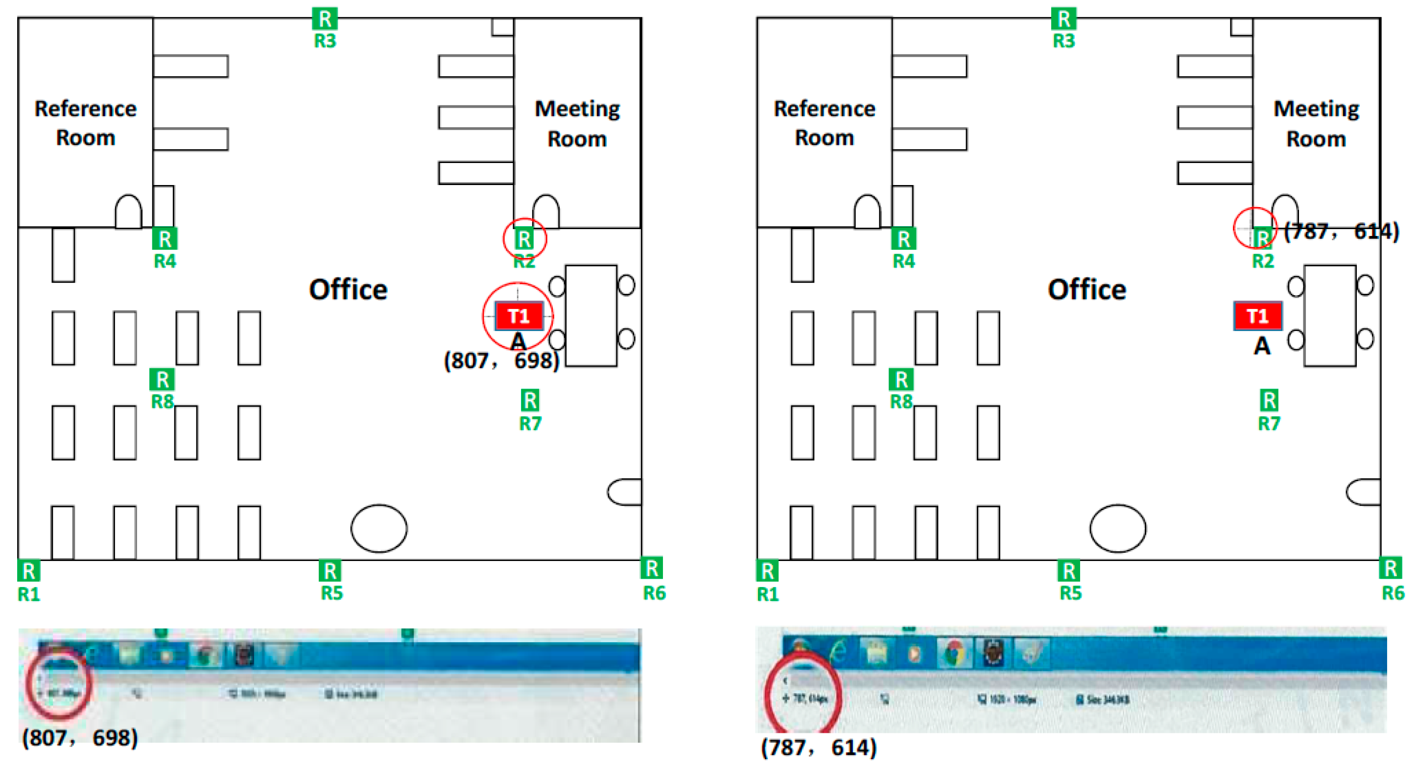
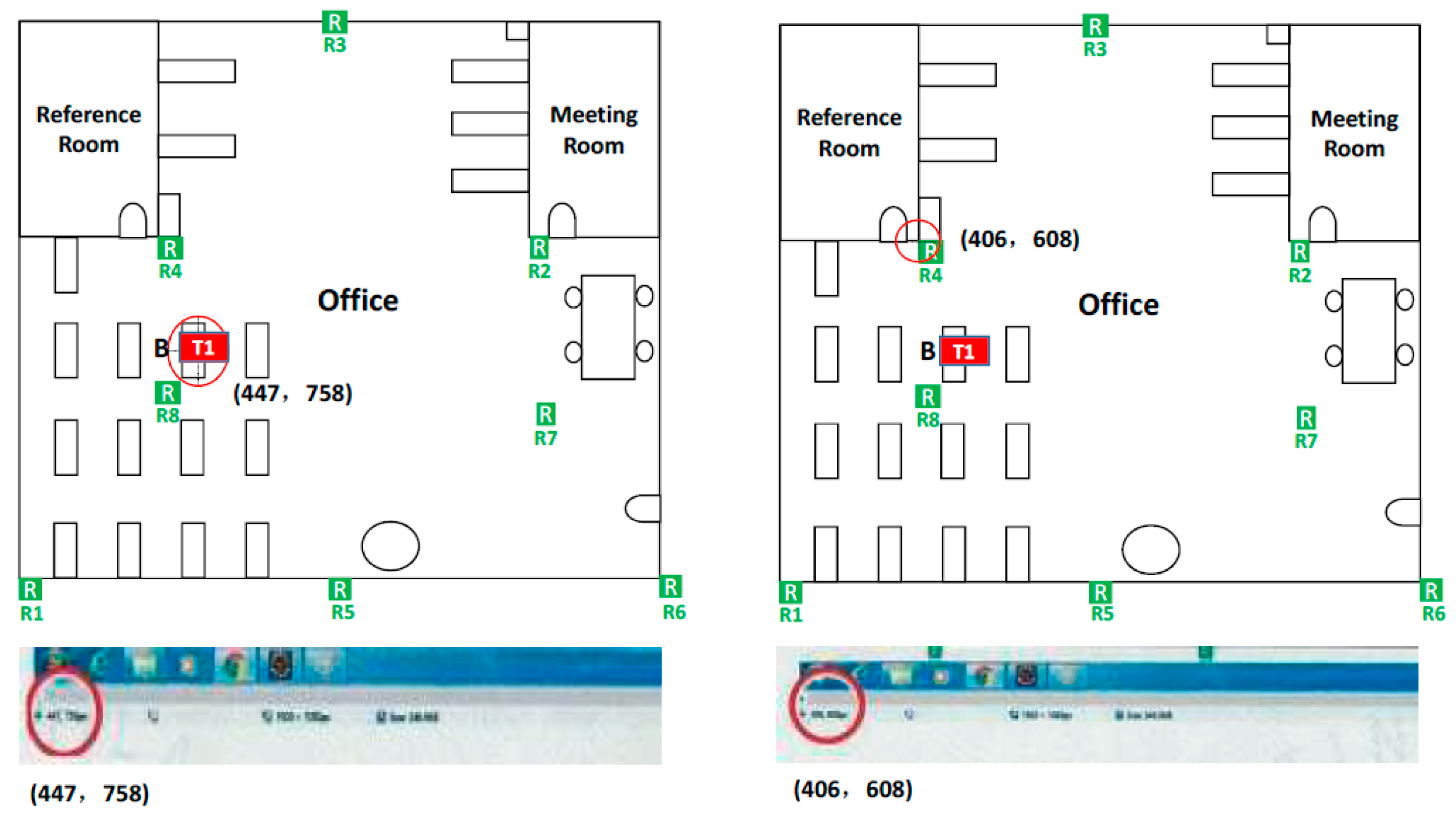
| 1 | (807, 698) | (787, 614) | (20, 84) | 1.296 | 1.9 | 0.594 | 0.541 |
| 2 | (615, 250) | (192, 448) | 7.311 | 8.3 | 0.788 | ||
| 3 | (410, 300) | (397, 398) | 8.432 | 9.0 | 0.567 | ||
| 4 | (452, 480) | (355, 218) | 6.248 | 6.8 | 0.655 | ||
| 5 | (447, 758) | (406, 608) | (41, 150) | 2.325 | 2.5 | 0.167 | |
| 6 | (154, 660) | (293, 98) | 4.634 | 4.8 | 0.165 | ||
| 7 | (260, 520) | (187, 238) | 4.540 | 4.9 | 0.359 | ||
| 8 | (280, 450) | (167, 308) | 5.255 | 5.9 | 0.744 |
© 2019 by the author. Licensee MDPI, Basel, Switzerland. This article is an open access article distributed under the terms and conditions of the Creative Commons Attribution (CC BY) license (http://creativecommons.org/licenses/by/4.0/).
Share and Cite
Bae, Y. Robust Localization for Robot and IoT Using RSSI. Energies 2019, 12, 2212. https://doi.org/10.3390/en12112212
Bae Y. Robust Localization for Robot and IoT Using RSSI. Energies. 2019; 12(11):2212. https://doi.org/10.3390/en12112212
Chicago/Turabian StyleBae, Youngchul. 2019. "Robust Localization for Robot and IoT Using RSSI" Energies 12, no. 11: 2212. https://doi.org/10.3390/en12112212
APA StyleBae, Y. (2019). Robust Localization for Robot and IoT Using RSSI. Energies, 12(11), 2212. https://doi.org/10.3390/en12112212