Integrated Energy and Thermal Management for Electrified Powertrains

Abstract

This study presents an integrated energy and thermal management system to identify the fuel-saving potential caused by cold-starting an electrified powertrain. In addition, it quantifies the benefit of adopting waste heat recovery (WHR) technologies on the ultimate fuel savings. A cold-start implies a low engine temperature, which increases the frictional power dissipation in the engine, leading to excess fuel usage. A dual-source WHR (DSWHR) system is employed to recuperate waste heat from exhaust gases. The energy harvested is stored in a battery and can be retrieved when needed. Moreover, the system recovers waste heat from an electric machine, including power electronics and a continuous variable transmission, to boost the heating performance of a heat pump for cabin heating. This results in a decrease in the load on the battery. The integrated energy and thermal management system aims at maximizing the fuel efficiency for a pre-defined drive cycle. Simulation results show that cold-start conditions affect the fuel-saving potential significantly, up to 7.1% on the New European Driving Cycle (NEDC), yet have a small impact on the optimal controller. The DSWHR system improves the fuel economy remarkably, up to 13.1% on the NEDC, from which the design of WHR technologies and dimensioning of powertrain components can be derived. As the optimal solution is obtained offline, a complete energy consumption minimization strategy framework, considering both energy and thermal aspects, is proposed to enable online implementation.

1. Introduction

Hybrid electric vehicles (HEVs), which provide opportunities for the improvement of fuel efficiency, are emerging to meet unprecedented emissions regulations and energy shortages. As HEVs use multiple power sources, of particular importance is the development of energy management systems (EMSs) for HEVs so as to maximize their fuel economy [1]. An EMS aims at controlling the power-flow of the hybrid powertrain in an optimal way; for example, the torque split between the internal combustion engine (ICE) and the electric machine (EM). In this respect, a vast amount of literature exists, including both offline and online control strategies, such as rule-based, dynamic programming (DP), Pontryagin’s minimum principle (PMP), and equivalent consumption minimization strategies (ECMS) [2,3,4,5]. Among these control strategies, DP is widely chosen as a good candidate for obtaining a global optimal solution, handling non-linear constraints, and assessing online controllers, as shown in [6]. Previous studies have been mainly concerned with only one continuous dynamic state, the state of charge (SOC) of the battery [7], which takes into consideration chemical, mechanical, and electrical energy flows. The thermal domain, however, which is also an integral part of an electrified powertrain and which influences energy control decisions, is yet to be investigated.

A majority of researchers currently design EMSs under the assumption that the engine is already at its operating temperature at the outset; namely, a warm-start [8]. This may not be realistic, and we may have the case where the vehicle has been parked for a few hours, resulting in a cold-start; which is common in the real world. Cold-start conditions imply a low engine temperature, which increases frictional losses in the engine, leading to excess fuel consumption due to high-viscosity effects and poor combustion. Furthermore, some official drive cycles—for instance, the New European Driving Cycle (NEDC) and the Worldwide Harmonized Light Vehicles Test Cycles (WLTC)—require cold-start conditions to measure fuel consumption [9]. The required starting temperature is far below the engine operating temperature. The impact is particularly high in the first few minutes of driving. Due to efficient and intermittent engine operation, this effect holds for a longer time in a hybrid powertrain than for its traditional equivalent. The difference in fuel consumption between a warm-start and a cold-start is regarded as the fuel-saving potential. It can be obtained by extending the design space of conventional EMSs with an extra continuous dynamic state, the engine temperature. The fuel-saving potential has been reported to be large (12% [10]) for the NEDC. It has also been shown, in [11], that cold-start conditions increase fuel consumption by up to 14.6% in the urban part of the NEDC, which well-represents the warm-up phase. However, few attempts can be found to close this gap; that is, to improve fuel efficiency with cold-start conditions and thereby quantify the ultimate fuel savings that could be realized in reality.

A numerical simulation was carried out to analyze energy losses of a plug-in HEV (PHEV), as illustrated in Figure A1. The goal of this simulation was to gain qualitative insights into areas where most of the fuel economy improvements could be obtained. The vehicle was subject to a cold-start, and the simulation was performed on the representative NEDC, assuming a sustained charge. This means the SOC of the battery at the beginning of a driving mission is equal to the SOC at the end of the trip, which implies that the battery is utilized as an energy buffer, and the energy is ultimately from the engine. It can be observed that the engine accounts for most of the energy losses. Therefore, achieving a high mechanical efficiency is crucial. A large part of the fuel energy is wasted into the surroundings, in the form of exhaust gases. Hence, recuperating a certain amount of that energy, which would otherwise be dissipated into the environment, is a promising way to improve powertrain efficiency. Two types of waste heat recovery (WHR) technologies can be found: Thermoelectric generators [12,13,14,15,16] and Rankine cycle-based WHR systems [17,18,19,20]. A thermoelectric generator consists of various P-type and N-type semiconductor materials, which convert heat into electricity directly, based on the Seebeck effect [21]. The Seebeck effect describes the voltage generated across the junctions of two dissimilar materials, owing to a temperature gradient. It has the advantages of no moving parts and no chemical reactions and, as long as there is a temperature difference, it produces electricity. Nevertheless, considering conversion efficiency, technical readiness, and cost, Rankine cycle systems are preferable. It has been shown that Rankine cycle systems have an efficiency of up to 15% [18,22,23,24]. A PMP-based energy management system for controlling Rankine cycle systems has been presented in [22]. Maximizing the power output of a Rankine cycle system on board a diesel-electric railcar has been reported in [24], by using DP and dynamic real-time optimization. Furthermore, [25] demonstrated a recovery efficiency of 10% for an electrified powertrain on the NEDC. Additionally, the turbine in a Rankine cycle system can be coupled with a generator, which constitutes a Rankine cycle-based electrical WHR system. From a control point of view, it is advantageous to store the recovered waste heat energy in the energy buffer. A Rankine cycle-based electrical WHR system is comprised of five main components: Evaporator, expander, generator, condenser, and pump, as shown in Figure A2. The working fluid is pumped from low pressure to high pressure, which then absorbs heat from exhaust gases through the evaporator and undergoes a phase change, from liquid to vapor. Expansion of the vaporized fluid subsequently produces mechanical energy by the expander, which is converted into an electrical form by the generator. The generated electricity is eventually stored in the energy buffer, which can be retrieved when needed. Consequently, the working fluid dissipates heat to the surroundings at the condenser and undergoes another phase change, from vapor to liquid. This technology is mainly adopted for internal combustion engine vehicles [26], although a few applications can be found in HEVs. Harvesting waste heat from exhaust gases is termed exhaust gas WHR (EGWHR).

It can also be seen that auxiliary power demand (cabin heating, in this case) consumes a significant amount of energy from the battery, which eventually leads to fuel consumption with charge sustenance. Obviously, using electricity from the battery directly, conventional electric heaters are not able to provide an economic solution. To reduce energy consumption, a heat pump (owing to higher coefficient of performance) has proved to be a promising alternative [27,28,29]. Traditionally, a heat pump only extracts heat from the outside air to heat the cabin. As is made evident by Figure A1, the amount of waste heat from power electronics and electric machine (PEEM) is significant as well. Recuperating a certain percentage of that power, which would otherwise be wasted ambiently, rather than using additional power from the battery, is a promising way to promote energy efficiency. More recently, in addition to ambient air, a heat pump makes use of the waste heat from PEEM [30]. It exchanges the heat with the refrigerant circuit and cabin heating system to boost heating performance, resulting in a decrease in battery load, as demonstrated in Figure A3. This, ultimately, contributes to fuel efficiency improvement. It has been reported that, by utilizing the waste heat from ambient and electric devices, the coefficient of performance and heating capacity increase by 9.3% and 31.5% [30], respectively. Heat pumps are mostly used in electric vehicles [31].

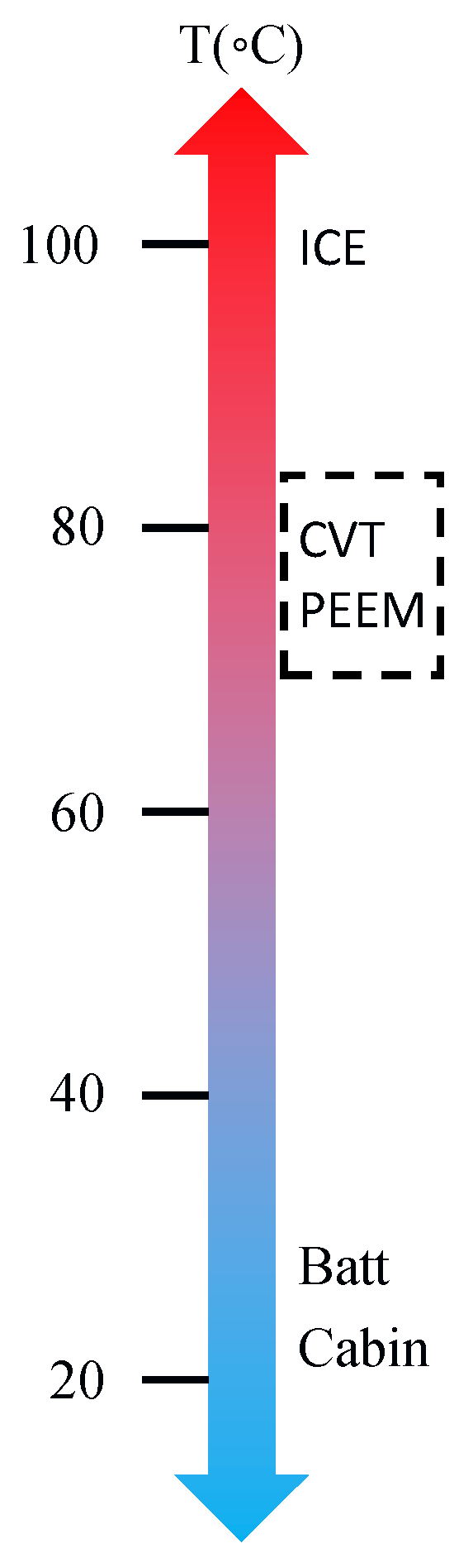
It is worth mentioning that a HEV, especially a PHEV, can be seen as a mixture of an internal combustion engine vehicle and an electric vehicle, which benefits from the technological advancements on both sides. Interestingly, a combination of these technologies—an EGWHR system and a heat pump extracting thermal energy from ambient and electric devices—have hardly been found in the PHEV context. Furthermore, observing the temperature levels of the major components of a CVT-based electrified powertrain, as shown in Figure A4, the PEEM can be integrated into the same housing as the CVT. They can be combined into a single heat source, by sharing the same cooling loop (e.g., with oil cooling) and contributing together to the heat which can be harvested by the heat pump, resulting in improved heating performance. Recuperating waste heat from PEEM and CVT is termed electric path WHR (EPWHR). A dual-source WHR (DSWHR) system is constituted of an EGWHR sub-system and an EPWHR sub-system.

Furthermore, it has been widely acknowledged that the optimal solution obtained from DP is not implementable. Moreover, earlier studies mainly focused on the transient behavior of powertrain components, when it comes to thermal aspects (e.g., heating up the component from a cold-start to its operating temperature) [32,33]. Afterwards, the operating temperature is assumed to be well maintained, which is actually the main goal of the corresponding thermal management system (TMS), in practice. It is obvious that the cooling system is not integrated and the cooling power consumption is neglected, which would influence the control strategy and the fuel consumption measurement. A systematic approach, based on optimal control theory, to facilitate an online implementation of complete energy and thermal management for electrified powertrains has not yet been developed.

In view of the above discussion, this work proposes an original integrated energy and thermal management system (IETMS) for electrified powertrains, in order to investigate the impact of cold-start conditions and the benefits of using the DSWHR system. Furthermore, a new complete energy consumption minimization strategy (CECMS) framework is presented, in order to minimize the complete energy flow; including both energy and thermal aspects. It achieves a close-to-optimal solution by taking advantages of DP, PMP, and ECMS algorithms. These results extend the work presented in [34]. The rest of this paper is organized as follows. The system model is given in Section 2. The optimization problem is formulated in Section 3. Section 4 presents the numerical results. A road map for designing the CECMS framework is shown in Section 5. Finally, the conclusions are drawn in Section 6.

2. System Modeling

The proposed integrated energy and thermal management system for a CVT-based PHEV is shown in Figure 1. PHEVs are best characterized by their charge-sustaining and charge-depleting modes. In this study, a charge-sustaining mode is assumed, as it is a common way to assess the performance of the control strategy [25,35]. The major components of the considered PHEV are the engine, battery, PE, EM, CVT, and vehicle. As can be seen from the figure, apart from traditional chemical, mechanical, and electrical energy flows, thermal energy (as indicated with the red-dashed lines) is added. In particular, the waste heat from the engine is recovered by the EGWHR sub-system, and the recovered power is stored into the battery. PEEM and CVT are combined, and the resulting waste heat is recuperated by the EPWHR sub-system, which reduces the load due to cabin heating demand on the battery. It can be observed that the vehicle has five different driving modes: Engine (ICE), charging (CH), electric vehicle (EV), motor assist (MA), and brake energy recuperation (BER). The ICE mode represents when only the engine is used to propel the vehicle. The CH mode indicates that the engine not only drives the wheels, but also charges the battery. The EV mode means that the EM is the only power source and the engine is off. The MA mode reflects when the EM is utilized to assist the engine to meet the driving demand. The BER mode is a mode where the braking energy is recuperated and stored into the battery. Detailed descriptions of these driving modes can be found in [36]. The electrified powertrain model is backward-facing (i.e., the drive cycle has to be known a priori), and includes both energy dynamics and thermodynamics. As far as the energy dynamics are concerned, the most relevant inertias are taken into account: The inertias of the engine, EM, variator in the CVT, and the vehicle. Some component models are represented by experimentally-based lookup tables, due to their non-linear behavior. In terms of thermodynamics, it is assumed that, except for the engine, the heat source components are in thermal equilibrium with the ambient conditions. The engine thermodynamics model, utilizing first principles [37], was developed on the basis of [33], in which the experiments were performed, and parameters are used where applicable. Once the engine temperature reaches its operating temperature, after which the cold effect on fuel consumption becomes negligible, the engine temperature is assumed to be kept at this reference. Therefore, the effect of the radiator and the cooling power consumption are neglected, which will be taken into account in Section 5.3 to design a CECMS. Kinematics, dynamics, and constraints are modeled with a discrete time-step of one second, which is sufficient for the design of the integrated energy and thermal controller. The key model parameters are listed in

Table 1. Main model parameters.

Parameter	Value	Unit	Description
$m_{veh}$	1600	kg	Vehicle mass
${\gamma }_{var,max}/{\gamma }_{var,min}$	7	-	Ratio coverage of continuous variable transmission
$T_{ice}$	239	Nm	Engine torque
$P_{ice}$	99	kW	Engine power
$T_{em,max}$	350	Nm	Peak torque of electric machine
$T_{em}$	210	Nm	Continuous torque of electric machine
$w_{em,max}$	7800	rpm	Maximum speed of electric machine
$P_{em,max}$	74	kW	Peak power of electric machine
$P_{em}$	50	kW	Continuous power of electric machine
$Q_{batt}$	40	Ah	Battery capacity
$V_{nom}$	3.75	V	Battery nominal voltage
$c_{ice}$	630	J/kgK	Engine specific heat
$c_h$	0.62	−	Engine heating coefficient
${\theta }_{ice,max}$	80	°C	Engine operating temperature
$c_{ice,1}$	0.0034	1/K	Engine cold factor coefficient
$c_{ice,2}$	0.016	1/K	Engine cold factor coefficient
$c_{exh,1}$	0.42	-	Exhaust gas fraction coefficient
$c_{exh,2}$	0.0002	s/rad	Exhaust gas fraction coefficient

[33,38]. The battery considered is a lithium-ion type battery with specific energy density of 113 Wh/Kg. The overall system can be expressed as

$$x(k+1)=f\left(x\right(k),u(k),w(k\left)\right),$$

(1)

where k is the time index. The disturbance vector $w\left(k\right)$ contains the vehicle speed and vehicle acceleration, which are provided by the drive cycle, given by

$$w\left(k\right)=\left[\begin{array}{c}{v}_{veh}\left(k\right)\\ a_{veh}\left(k\right)\end{array}\right].$$

(2)

The control vector $u\left(k\right)$ consists of the variator ratio of the CVT and the torque split factor describing the torque split between the EM and the engine, giving

$$u\left(k\right)=\left[\begin{array}{c}{\gamma }_{var}\left(k\right)\\ u_{ts}\left(k\right)\end{array}\right].$$

(3)

The state variables $x\left(k\right)$ are the SOC of the battery, which represents the energy dynamics, and the engine temperature, which reflects the thermodynamics; that is,

$$x\left(k\right)=\left[\begin{array}{c}\xi \left(k\right)\\ {\theta }_{ice}\left(k\right)\end{array}\right].$$

(4)

2.1. Driving Profile

As reported in [39], the average European driving distance is 10 km. The NEDC, an official driving profile which is commonly used to certify fuel consumption measurements, has a duration of 1180 s and a length of 11 km. Moreover, it well-captures the transient behavior of the engine, which is the main focus of this research. Therefore, the NEDC was selected as the input for the optimization problem in this study. Notice that, for other drive cycles, although the quantity might vary, the methodology presented also applies.

2.2. Longitudinal Dynamics

Considering aerodynamic drag force, rolling resistance, and inertia force, the wheel speed $w_{wh}\left(k\right)$ and torque $T_{wh}\left(k\right)$ required to follow the drive cycle, which is represented by vehicle velocity $v_{veh}$ and acceleration $a_{veh}$, can be expressed as follows:

$$w_{wh}\left(k\right)=\frac{v_{veh}\left(k\right)}{r_{wh}},$$

(5)

$$T_{wh}\left(k\right)=(\frac{1}{2}·\rho ·c_d·A·v_{veh}^2\left(k\right)+c_r·m_{veh}·g·sign\left(v_{veh}\left(k\right)\right)+(m_{veh}+4·\frac{J_{wh}}{r_{wh}^2})·a_{veh}\left(k\right))·r_{wh},$$

(6)

where $\rho$ is the density of air, $c_d$ the aerodynamic drag coefficient, A the frontal area of the vehicle, $c_r$ the rolling resistance coefficient, $m_{veh}$ the vehicle mass, g the gravitational acceleration, $J_{wh}$ the wheel inertia, and $r_{wh}$ the effective wheel radius.

2.3. Continuous Variable Transmission

The push-belt CVT is made up of four main parts: Variator, pump, DNR (drive, neutral, and reverse), and final drive. It provides a continuous variable speed ratio ${\gamma }_{var}$ between the primary pulley and the secondary pulley. This allows the engine speed to be decoupled from the wheel speed, in order to optimize the operating point of the engine. It should be noted that pump speeds below 1000 rpm are prohibited. Given the required torque and speed at the wheels, the speed and torque of the final drive are obtained by

$$w_{fd}\left(k\right)=w_{wh}\left(k\right)·{\gamma }_{fd},$$

(7)

$$T_{fd}\left(k\right)=\left\{\begin{array}{cc}\frac{T_{wh}\left(k\right)}{{\eta }_{fd}·{\gamma }_{fd}},\hfill & \mathrm{if}{T}_{wh}\left(k\right)>0,\hfill \\ \frac{{\eta }_{fd}·T_{wh}\left(k\right)}{{\gamma }_{fd}},\hfill & \mathrm{if}{T}_{wh}\left(k\right)\le 0,\hfill \end{array}\right.$$

(8)

where ${\gamma }_{fd}$ is a constant ratio between the secondary pulley and the wheel and ${\eta }_{fd}$ is the efficiency of the final drive. Taking into consideration the inertia effects $J_{var,i}$ and $J_{var,o}$, the speed and torque of the primary pulley are calculated by

$$w_{pri}\left(k\right)=w_{wh}\left(k\right)·{\gamma }_{fd}·{\gamma }_{var}\left(k\right),$$

(9)

$$T_{pri}\left(k\right)=J_{var,i}·\Delta w_{pri}\left(k\right)+\frac{J_{var,o}·\Delta w_{fd}\left(k\right)+T_{fd}\left(k\right)}{{\gamma }_{var}\left(k\right)},$$

(10)

where $\Delta w_{fd}$ and $\Delta w_{pri}$ are the rotational acceleration of the final drive and the primary pulley, respectively. The total torque demand is thus given by

$$T_{dem}\left(k\right)=T_{loss}(w_{pri}\left(k\right),T_{pri}\left(k\right),{\gamma }_{var}\left(k\right))+T_{pri}\left(k\right),$$

(11)

where $T_{loss}(w_{pri},T_{pri},{\gamma }_{var})$ represents the torque loss in the CVT, consisting of the torque loss in the DNR, pump, and variator, which are computed using detailed loss-maps based on measurement data. Bounds on the variator ratio and the primary pulley torque are

$${\gamma }_{var}\left(k\right)\in [{\gamma }_{var,min},{\gamma }_{var,max}],$$

(12)

$$T_{pri}\left(k\right)\in [T_{pri,min},T_{pri,max}].$$

(13)

Constraints on the primary pulley speed will be implicitly considered in the constraints on the engine speed.

2.4. Torque Split

The torque split between the EM and the engine is determined by the torque split factor $u_{ts}$. Given the total torque request, the torque provided by the engine and EM are expressed as

$$T_{ice,ts}\left(k\right)=(1-u_{ts}\left(k\right))·T_{dem}\left(k\right),\mathrm{if}{T}_{dem}\left(k\right)>0,$$

(14)

$$T_{em,ts}\left(k\right)=u_{ts}\left(k\right)·T_{dem}\left(k\right),\mathrm{if}{T}_{dem}\left(k\right)>0\vee T_{dem}\left(k\right)\le 0\wedge w_{pri}\left(k\right)\ge \frac{1000·\pi }{30}.$$

(15)

Taking into account the constraints on the EM, battery, and charge sustenance, the additional torque supplied by mechanical braking is written as

$$T_{br}\left(k\right)=T_{dem}\left(k\right)-T_{em,ts}\left(k\right),\mathrm{if}{T}_{dem}\left(k\right)<0.$$

(16)

The torque split factor is limited by

$$u_{ts}\left(k\right)\in [u_{ts,min},u_{ts,max}],$$

(17)

where $u_{ts,max}=1$ and $u_{ts,min}<0$, depending on the engine size. The relationship between the driving modes and the torque split factor can be summarized as follows: When $u_{ts}=1$, it indicates that the engine is shut off and either the EV or BER mode is activated (depending on the torque demand). The car is in the MA mode if $0<u_{ts}<1$, and $u_{ts}=0$ represents that the ICE mode is active. The vehicle is in the CH mode if $u_{ts}<0$, with $u_{ts}=u_{ts,min}$ representing full recharge.

2.5. Internal Combustion Engine

In the considered PHEV, the crankshaft of the engine is coupled to the primary pulley shaft directly, which implies that the engine speed is equal to the primary pulley speed. Moreover, engine speeds below 1000 rpm are prevented. In consideration of the engine inertia, the speed and torque of the engine are given by

$$w_{ice}\left(k\right)=w_{pri}\left(k\right),\mathrm{if}{T}_{ice}\left(k\right)>0,$$

(18)

$$T_{ice}\left(k\right)=J_{ice}·\Delta w_{pri}\left(k\right)+T_{ice,ts}\left(k\right).$$

(19)

With warm-start conditions, a lookup table is utilized to obtain the fuel consumption represented by the injected fuel mass flow $\Delta m_f\left(k\right)$, giving

$$\Delta m_f\left(k\right)=\Delta m_f(w_{ice}\left(k\right),T_{ice}\left(k\right)).$$

(20)

The engine speed and torque are subject to the lower and upper limits

$$w_{ice}\left(k\right)\in [w_{ice,min},w_{ice,max}],$$

(21)

$$T_{ice}\left(k\right)\in [T_{ice,min}\left(w_{ice}\left(k\right)\right),T_{ice,max}\left(w_{ice}\left(k\right)\right)].$$

(22)

Subsequently, the consumed fuel power is calculated by

$$P_f\left(k\right)=\Delta m_f\left(k\right)·H_{lhv},$$

(23)

where $H_{lhv}$ is the lower heating value of gasoline. With cold-start conditions, however, because of higher frictional losses, the fuel consumption is higher than that of a warm-start. In order to mimic the real situation, an engine cold factor is introduced to adjust the nominal fuel power $P_f$, which is a function of the engine temperature that is always greater than or equal to one. The engine cold factor is defined as

$$c\left({\theta }_{ice}\left(k\right)\right)=\left\{\begin{array}{cc}1+c_{ice,1}·({\theta }_{ice,max}-{\theta }_{ice}\left(k\right))·e^{c_{ice,2}·({\theta }_{ice,max}-{\theta }_{ice}\left(k\right))},\hfill & \mathrm{if}{\theta }_{ice}\left(k\right)<{\theta }_{ice,max},\hfill \\ 1,\hfill & \mathrm{if}{\theta }_{ice}\left(k\right)={\theta }_{ice,max},\hfill \end{array}\right.$$

(24)

where $c_{ice,1}$ and $c_{ice,2}$ are the cold factor coefficients to correct the nominal fuel consumption, which are fitted parameters that are experimentally identified; and ${\theta }_{ice,max}$ is the operating temperature. Therefore, the temperature-dependent fuel power is calculated by

$$P_{che}\left(k\right)=c\left({\theta }_{ice}\left(k\right)\right)·P_f\left(k\right).$$

(25)

A significant portion of the fuel power is converted into mechanical power $P_{ice}$ to propel the vehicle, whereas another large part is wasted as the exhaust gases $P_{exh}$, followed by a relatively small power dissipation; that is, convection to the ambient air $P_a$. The remainder of the power is converted into heat, given by

$$P_{th}\left(k\right)=P_{che}\left(k\right)-P_{ice}\left(k\right)-P_{exh}\left(k\right)-P_a\left(k\right).$$

(26)

The mechanical power produced is obtained by

$$P_{ice}\left(k\right)=w_{ice}\left(k\right)·T_{ice}\left(k\right).$$

(27)

The exhaust gas heat is approximated as a function of the injected chemical power and the engine speed; that is,

$$P_{exh}\left(k\right)=(c_{exh,1}-c_{exh,2}·w_{ice}\left(k\right))·P_{che}\left(k\right),$$

(28)

where $c_{exh,1}$ and $c_{exh,2}$ are the exhaust gas fraction coefficients to estimate the engine speed-dependent exhaust gas power, as described in [40]; and $P_{exh}$ decreases with $w_{ice}$ linearly. The convection to the ambient air is given by

$$P_a\left(k\right)=c_a·A_{ice}·({\theta }_{ice}\left(k\right)-{\theta }_{amb}),$$

(29)

where $c_a$ is the heat transfer coefficient to the ambient air, $A_{ice}$ the heat exchange area, and ${\theta }_{amb}$ the ambient temperature. Therefore, the engine temperature can be calculated by

$${\dot{\theta }}_{ice}\left(k\right)=\left\{\begin{array}{cc}\frac{P_{th}\left(k\right)}{C_{ice}},\hfill & \mathrm{if}{\theta }_{ice}\left(k\right)<{\theta }_{ice,max},\hfill \\ 0,\hfill & \mathrm{if}{\theta }_{ice}\left(k\right)={\theta }_{ice,max},\hfill \end{array}\right.$$

(30)

where $C_{ice}$ is the engine heat capacity, given by

$$C_{ice}=c_h·c_{ice}·m_{ice},$$

(31)

where $c_h$ is a heating coefficient, which compensates for the slower heating of the metal parts than that of lubrication oil; $c_{ice}$ is the engine specific heat; and $m_{ice}$ is its mass.

2.6. Exhaust Gas Waste Heat Recovery

As shown in Figure A2, the EGWHR sub-system is utilized to recuperate a certain amount of the exhaust gas power $P_{exh}$ with recovery efficiency ${\eta }_{whr,eg}$, and the recuperated power $P_{whr,eg}$ is eventually stored in the battery. As the objective of this study is to gain qualitative insights into the order of fuel savings that could be achieved, a detailed EGWHR model is not developed. A black-box approach is adopted instead [41], where a lumped efficiency [42] taking into account of the efficiencies of all the components of the EGWHR sub-system [43] is used, and the maximum efficiency is 10% [25]. The EGWHR model is described as

$$P_{whr,eg}\left(k\right)={\eta }_{whr,eg}·P_{exh}\left(k\right),$$

(32)

where ${\eta }_{whr,eg}\in [0,10\%]$.

2.7. Integrated Motor-Generator

The EM employed is a permanent magnet synchronous motor (PMSM), which is an integrated motor-generator (IMG). It is linked to the input shaft of the CVT directly. Taking the EM inertia into account, the speed and torque of the EM are obtained by

$$w_{em}\left(k\right)=max(w_{pri}\left(k\right),\frac{1000·\pi }{30}),\mathrm{if}{w}_{pri}\left(k\right)>0,$$

(33)

$$T_{em}\left(k\right)=J_{em}·\Delta w_{em}\left(k\right)+T_{em,ts}\left(k\right).$$

(34)

The mechanical power generated by the EM is, then, calculated by

$$P_{em}\left(k\right)=w_{em}\left(k\right)·T_{em}\left(k\right).$$

(35)

A lookup table is used to describe the power loss of the EM, including PE:

$$P_{em,loss}\left(k\right)=P_{em,loss}(w_{em}\left(k\right),T_{em}\left(k\right)).$$

(36)

Consequently, the electrical power supplied to/by the EM is given by

$$P_{em,elec}\left(k\right)=P_{em}\left(k\right)+P_{em,loss}\left(k\right).$$

(37)

The constraints on the EM are

$$w_{em}\left(k\right)\in [w_{em,min},w_{em,max}],$$

(38)

$$T_{em}\left(k\right)\in [T_{em,min}\left(w_{em}\left(k\right)\right),T_{em,max}\left(w_{em}\left(k\right)\right].$$

(39)

2.8. Electric Path Waste Heat Recovery

The total heat production from the CVT and the EM—namely, the electric path—can be computed by

$$P_{ep}\left(k\right)=P_{em,loss}\left(k\right)+P_{cvt,loss}\left(k\right),$$

(40)

where $P_{cvt,loss}\left(k\right)$ is derived as follows:

$$P_{cvt,loss}\left(k\right)=P_{loss}(w_{pri}\left(k\right),T_{pri}\left(k\right),{\gamma }_{var}\left(k\right))+P_{fd,loss}\left(k\right),$$

(41)

where $P_{fd,loss}$ is the power loss of the final drive. As illustrated in Figure A3, the EPWHR sub-system is employed to recover a certain percentage of the waste heat $P_{ep}$ with recuperation efficiency ${\eta }_{whr,ep}$, and the waste heat harvested $P_{whr,ep}$ ultimately reduces the load on the battery. For the sake of simplicity and to obtain qualitative insights, this work assumes a lumped efficiency [42] considering heat exchange between the systems, where the maximum efficiency is 20% [30,44,45]. The reason for this is that, first of all, liquid-to-liquid heat exchange is relatively efficient (e.g., when using a liquid to liquid counter-flow plate fin heat exchanger) [46]. Furthermore, with proper arrangement of the heat exchangers in the electric path cooling circuit, heat pump, and the cabin heater system, the heat exchange can be efficient [44]. The EPWHR model is given by

$$P_{whr,ep}\left(k\right)={\eta }_{whr,ep}·P_{ep}\left(k\right),$$

(42)

where ${\eta }_{whr,ep}\in [0,20\%]$.

2.9. Cabin

For the purpose of this study, identifying the cost of cold-start conditions on the fuel usage and the benefits of adopting a DSWHR system, a detailed cabin model is not considered. Instead, the auxiliary power demand, represented by the cabin heating request, is assumed to take a constant value [27]; that is,

$$P_{aux}=1\left(kW\right).$$

(43)

The cabin heating power is provided by the battery. In charge-sustaining mode, eventually, this leads to fuel consumption.

2.10. Energy Buffer

The battery is modeled by using an equivalent circuit approach; that is, a voltage source in series with an internal resistance. The electric power supplied by the battery is obtained by

$$P_{batt}\left(k\right)=P_{em,elec}\left(k\right)+P_{aux}.$$

(44)

The battery current is, then, calculated by

$$I_{batt}\left(k\right)=\frac{V_{oc}\left(k\right)-\sqrt{V_{oc}^2\left(k\right)-4·P_{batt}\left(k\right)·R_{int}\left(k\right)}}{2R_{int}\left(k\right)},$$

(45)

where $V_{oc}$ is the open circuit voltage of the battery and $R_{int}$ is its internal resistance. Both $V_{oc}$ and $R_{int}$ are described by lookup tables, which are functions of the SOC. Consequently, the battery SOC is given by

$$\xi (k+1)=-\frac{{\eta }_{batt}\left(I_{batt}\left(k\right)\right)·I_{batt}\left(k\right)}{3600·Q_{batt}}\Delta t+\xi \left(k\right),$$

(46)

where ${\eta }_{batt}$ is the battery charging efficiency and $Q_{batt}$ is the battery capacity. The battery current is bounded by

$$I_{batt}\left(k\right)\in [I_{batt,min},I_{batt,max}].$$

(47)

3. Numerical Optimization

In this study, the engine is not only a power source to propel the wheels, but also a thermal accumulator. It accumulates thermal energy to bring its temperature to the operating temperature as fast as possible, so as to reduce the cold penalty, as reflected by (25). Moreover, the battery is regarded as an energy storage system, which stores energy from other sources and exchanges energy with the driven load. In addition to the five driving modes mentioned earlier, this paper introduces two thermal-related modes: ICE-Heating (ICEH) and waste heat recovery (WHR):

ICEH 

The engine temperature is lower than its efficient operating temperature, which implies a cold-start. The engine thermal energy level is lower than the desired level, and thermal energy is accumulated by the thermal accumulator.

WHR 

The recuperated energy from the exhaust gases is stored in the battery, which increases the energy content of the battery and can be retrieved for propulsion when needed. The recovered power from the electric path results in a decrease in battery load for cabin heating.

Due to the cold-start, the engine has to generate heat to warm up itself during the ICEH mode to reduce the cold effect, leading to an additional fuel cost. The additional fuel cost represents the fuel-saving potential, which shows the difference between a cold-start and a warm-start; essentially, the cost of the ICEH mode. Previously, with charge sustenance, the energy used in the MA and EV modes eventually came from the CH and BER modes. Now, the energy harvested from the WHR mode reduces the battery load directly, and can also be utilized for the MA and EV modes, resulting in extra fuel savings. The extra fuel savings indicates the ultimate fuel savings in reality, which demonstrates the discrepancy between a cold-start and a cold-start with DSWHR; essentially, the benefit of the WHR mode. It is clear that there is a trade-off between the ICE heating, and hence the cost on the fuel usage, and the utilization of the DSWHR system, and thus the gain on the fuel economy. To be more specific, in the presence of cold-start conditions, the IETMS attempts to generate not only an optimal SOC profile but also an ideal warm-up trajectory of the engine. This is achieved by controlling the driving modes and the ICEH mode. The fuel-saving potential can then be identified. Featuring the DSWHR, the IETMS aims to minimize the overall fuel consumption by optimally determining the driving modes and the thermal-related modes; namely, the ICEH and WHR modes. The ultimate fuel savings can, thus, be quantified. Although DP is an offline optimization method, it provides insights into the design of online implementable strategies. Given a drive cycle starting at $k_0$ and ending at $k_n$, DP [47,48], which uses Bellman’s principle of optimality, is applied to obtain optimal control inputs, by minimizing the objective function

$$\mathcal{J}=\sum _{k_0}^{k_{n-1}}\left[1+c_{ice,1}·({\theta }_{ice,max}-{\theta }_{ice}\left(k\right))·e^{c_{ice,2}·({\theta }_{ice,max}-{\theta }_{ice}\left(k\right))}\right]·\Delta m_f\left(k\right).$$

(48)

The optimal control inputs are represented by the variator ratio ${\gamma }_{var}$ and the torque split factor $u_{ts}$. The optimal control inputs, decided by the optimization algorithm, determine the driving mode (as defined in Section 2) and the thermal-related mode (as introduced above). Apart from the constraints described in Section 2, additional constraints on the system dynamic states are

$$\xi \left(k_0\right)=\xi \left(k_{n-1}\right),$$

(49)

$$\xi \left(k\right)\in [{\xi }_{min},{\xi }_{max}],$$

(50)

$${\theta }_{ice}\left(k\right)\in [{\theta }_{ice,min},{\theta }_{ice,max}].$$

(51)

Equation (49) ensures charge-sustaining. Recall that the aim of this study is to quantify the fuel-saving potential caused by cold-start conditions and the ultimate fuel savings contributed by the DSWHR system. Therefore, the numerical optimization problem given by (48) is solved for three simulation settings, which are described as follows:

S₀

The engine is already at its efficient operating temperature at the outset, which indicates that there is no cold impact. This is the ideal scenario. The system has only one continuous dynamic state, the SOC of the battery, and the energy controller aims at finding an optimal SOC trajectory;

S₁

The engine is subject to a cold-start, which is a common case in reality. The optimization problem contains two continuous dynamic states, being the SOC of the battery and the engine temperature. The optimization strategy attempts to generate an optimal SOC profile and an ideal warm-up trajectory of the engine simultaneously, by taking into account the ICEH mode; and

S₂

On the basis of $S_1$, the DSWHR system with ${\eta }_{whr,eg}=10\%$ and ${\eta }_{whr,ep}=20\%$ is included. The IETMS aims to maximize the overall fuel efficiency by striking a balance between the driving modes, ICEH mode and the WHR mode.

It should be noted that $S_1$ does not include the DSWHR system, which is the main difference from $S_2$. The fuel-saving potential can be obtained by comparing the results between $S_0$ and $S_1$. With the aid of the WHR technologies, $S_2$ attempts to bridge the gap between $S_0$ and $S_1$. By comparing the outputs from $S_1$ and $S_2$, the ultimate fuel savings can be quantified, which shows the upper bound of what can be achieved in practice.

4. Numerical Results and Discussion

The results for the integrated energy and thermal management in the electrified powertrain for the NEDC are shown in detail in Figure 2. The NEDC consists of an urban portion ([0, 780] s), where the driving load is low, and a highway part ([780, 1180] s), which features a high power demand. Obviously, all the strategies use the BER mode as much as possible to charge the battery, because braking energy is considered to be free energy. Generally, inefficient engine operation in low driving conditions restricts the driving mode in the urban region to the EV mode, especially the first 160 s. The battery propels the wheels, leading to a decrease in the SOC. This also reveals the fact that a PHEV is characterized by a big battery pack, which alone is able to satisfy the driving demand. Less frequent engine operation results in a slow rise of the engine temperature, which increases the cold impact on the fuel consumption. The highway section, in contrast, is mainly dominated by the CH mode, where engine driving is preferred. The engine drives the vehicle and charges the battery, which increases the SOC to meet the final constraint, due to charge sustaining. This results in a rapid rise of engine temperature, which decreases the cold effect on the fuel usage. Overall, however, intermittent and efficient engine operation prevents the engine from heating up fast. It is clear that the engine operating temperature is reached almost at the end of the drive cycle, around 994 s, which confirms the significance of considering the cold impact. It is, therefore, imperative to alleviate this situation. Surprisingly, the heating time of the engine in $S_2$ was longer than that in both $S_0$ and $S_1$. This is because the recuperated power from the EPWHR sub-system reduces the load on the battery, thus reducing the power needed for charging, as made evident by Figure 3. Note that, because of the resolution, the SOC trajectory appears to be a straight line. Moreover, the power recovered from the EGWHR sub-system is stored into the battery temporarily and utilized efficiently at high driving load, resulting in significant fuel consumption reduction. However, the impact of the cold-start on the integrated energy and thermal controller is small. The reason for this is that the optimal strategy aims at minimizing the energy loss of the engine, which is found to be similar in all of the cases. This is in accordance with the observation as above, where the engine accounts for most of the losses of a PHEV and maintaining a high engine efficiency plays an important role. It also explains the similarities between $S_0$ and $S_1$, in terms of hybrid mode visualization. As a result, a cold-start had a substantial influence on the fuel usage (7.1% on the NEDC) and the DSWHR system had a significant improvement on the fuel efficiency (13.1% on the NEDC). On average, the recovered power from the exhaust gases was 523 W and from the electric path was 225 W. Clearly, the gain of the WHR mode outperforms the pay of the ICEH mode, to a large extent. It should be noted that the heating time of the engine and the energy that can be recovered from the DSWHR system are dependent on driving conditions.

4.1. Influence of Driving Conditions

In order to investigate the effect of the driving scenario, the real-world WLTC was used for comparison purposes. In the WLTC, the engine temperature increases faster—in particular, in the beginning phase—which reduces the cold impact substantially, as shown in Figure 4. The heating time of the engine is 860 s. This is best explained by the fact that the WLTC is more aggressive than the NEDC. As this work primarily concentrates on the transient behavior of the engine, the first 780 s was chosen for both driving cycles, for fair comparison. It can be seen that, first of all, the average speed of the WLTC is (slightly) higher than that of the NEDC. Moreover, the engine-on time was significantly longer in the WLTC. Additionally, the percentage of high driving power demand in the WLTC is significantly higher than that in the NEDC. The percentage of high driving power demand is defined as the time instants in which $P_{dem}\left(k\right)>10kW$, with respect to the duration of the drive cycle. The propulsion power is given by

$$P_{dem}\left(k\right)=(\frac{1}{2}·\rho ·c_d·A·v_{veh}^2\left(k\right)+c_r·m_{veh}·g·sign\left(v_{veh}\left(k\right)\right)+(m_{veh}+4·\frac{J_{wh}}{r_{wh}^2})·a_{veh}\left(k\right))·v_{veh}\left(k\right).$$

(52)

It can be inferred that, as the cold effect was reduced, the fuel-saving potential on the WLTC was much less than that on the NEDC. Furthermore, the WLTC contained more opportunities for recovering waste heat, which resulted in larger fuel savings. Even though the WLTC represents real-world driving behavior, for the purpose of this study—considering cold-start conditions and engine thermodynamics under transient operating conditions—the NEDC is more representative. This is in accordance with the assumptions made before, where the heating period was taken into account and the effect of the radiator was neglected. For the WLTC, these assumptions do not hold, as the operating temperature was reached at 860 s with respect to the total duration of 1800 s and the radiator would have had a significant influence on the energy consumption. Therefore, the NEDC was used for further analysis.

For the NEDC, it can also be observed that the average speed of the urban part is much lower than that of the highway section. For the DSWHR system, the average recuperated power was 338 W for urban conditions, while it was 1550 W for the highway situations. As the optimal controller aims to maintain a high engine mechanical efficiency, it is expected that, as the average speed increases, the waste heat power that can be recovered increases. Notice that the fuel-saving potential obtained from the NEDC is representative for similar driving scenarios; for example, the Japan Cycle ’08 (JC08) and the urban part of the Common Artemis Driving Cycle (CADC). These drive cycles have similar durations and average speeds for the urban sections, where the engine transient behavior is well-captured. The ultimate fuel savings from the NEDC is applicable to drive cycles that have similar speed trends. More importantly, the methodology introduced in this study works the same for other drive cycles.

4.2. Analysis of Engine Temperature

It should be noted that the 7.1% fuel-saving potential on the NEDC was identified when the initial engine temperature was 20 °C. In practice, the fuel-saving potential varies; for example, depending on how long the car has been parked. The fuel economy improvement rate can be expressed as

$$\Delta F{S}_{{\theta }_{ice}\left(k_0\right)}=\frac{FC{|}_{{\theta }_{ice}\left(k_0\right)=20°}-F{C}_{{\theta }_{ice}\left(k_0\right)}}{FC{|}_{{\theta }_{ice}\left(k_0\right)=20°}},$$

(53)

where ${\theta }_{ice}\left(k_0\right)\in [20°,80°]$ represents the initial engine temperature. As illustrated in Figure 5, the relationship between the initial engine temperature and the fuel efficiency improvement rate can be approximated by a quadratic function as follows,

$$\Delta F{S}_{{\theta }_{ice}\left(k_0\right)}=c_1·{\theta }_{ice}^2\left(k_0\right)+c_2·{\theta }_{ice}\left(k_0\right)+c_3,$$

(54)

with $c_1=-0.0015$, $c_2=0.2739$, and $c_3=-4.9$. It can be seen that the fuel economy increases while increasing the initial engine temperature, due to the cold factor (24). Given an initial engine temperature, the corresponding fuel-saving potential can be computed. The required thermal budget that the system should provide to bring the engine from an initial thermal state to the desired thermal energy level is estimated by

$$E_{th}=C_{ice}·({\theta }_{ice,max}-{\theta }_{ice}\left(k_0\right)),$$

(55)

where $E_{th}$ is a constant value, independent of drive cycles. It is only related to a specific engine and its initial engine temperature. As long as the system can allocate the demanded thermal energy to heat the engine, the impact of a cold-start on the fuel consumption can be reduced. Using waste heat from the electric path to warm up the engine during pure electric driving is a case in point.

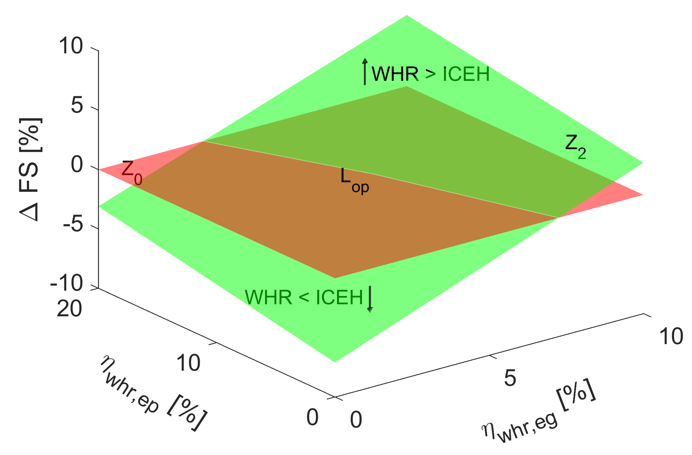
4.3. Effect of DSWHR Efficiencies

Notice that the 13.1% fuel efficiency improvement on the NEDC was achieved with maximum recovering efficiencies, which may not be economically feasible in practice. The relative fuel savings, represented by the surface $Z_2$, with different efficiencies of the DSWHR system (i.e., ${\eta }_{whr,eg}\times {\eta }_{whr,ep}$), is shown in Figure 6. The relative fuel savings is calculated by

$$\Delta FS=\frac{F{C}_{S_0}-F{C}_{S_2}}{F{C}_{S_1}},$$

(56)

where $F{C}_{S_0}$, $F{C}_{S_1}$, and $F{C}_{S_2}$ are the fuel consumptions of $S_0$, $S_1$, and $S_2$, respectively. The part of $Z_2$ above $Z_0$ implies that the recuperated energy was able to cover the heating energy required; namely, $WHR>ICEH$. The part of $Z_2$ below $Z_0$ indicates that the recovered benefit was not sufficient enough to pay for the heating cost; namely, $WHR<ICEH$. The surface $Z_0=0$ is determined by $\Delta FS=0$. The intersection $L_{op}$ represents the combinations of harvesting efficiencies that satisfy $\Delta FS=0$—namely, $WHR=ICEH$—which means that the heating cost was compensated for by the energy harvested. It can be inferred, from $WHR=ICEH$, that, in reality, with a small EGWHR sub-system and a small EPWHR sub-system, the fuel efficiency can be improved remarkably. It achieves the same fuel economy as the ideal warm-start condition, which serves as the first step towards the design of WHR technologies. Furthermore, it provides insights into the sizing of electrified powertrain components. For example, the recovered power from the DSWHR system can downsize the battery pack.

5. Towards an Online Implementable Strategy

It is known that the computation time of DP increases exponentially with the number of states (e.g., thermal states), the so-called curse of dimensionality [47]. Furthermore, DP demands that the driving profile is known a priori, which is not implementable. In real situations, driving conditions are not available in advance, which requires the control strategy to calculate the solution online. Therefore, it is important to devise an online implementable strategy that preserves optimality, taking into consideration both energy and thermal aspects. This is realized by establishing relationships between DP, PMP, and ECMS.

5.1. Dynamic Programming

DP offers sufficient conditions for the global optimality and provides insights into the design of an online energy and thermal management system. In DP, the optimal control policy is found using an exhaustive search by evaluating the following value function, referring to (48), in which the dynamic states are embedded,

$$\begin{array}{cc}\underset{u\left(k\right)\in \mathcal{U}}{min}:\mathcal{J}(x\left(k\right),k)=\{\hfill & G(x\left(k_n\right),k_n)+\hfill \\ & {\displaystyle \sum _{k_0}^{k_{n-1}}}(1+c_{ice,1}·({\theta }_{ice,max}-{\theta }_{ice}\left(k\right))·e^{c_{ice,2}·({\theta }_{ice,max}-{\theta }_{ice}\left(k\right))})·\Delta m_f\left(k\right)·\Delta t·H_{lhv}\},\hfill \end{array}$$

(57)

where $\mathcal{U}$ represents the admissible controls and $G(x\left(k_n\right),k_n)$ represents the terminal cost. The intermediate cost can be calculated by

$$\begin{array}{cc}\mathcal{J}(x\left(k\right),k)=\underset{u\left(k\right)\in \mathcal{U}}{min}\{\hfill & \mathcal{J}\left(x\right(k+1),k+1)+\hfill \\ & (1+c_{ice,1}·({\theta }_{ice,max}-{\theta }_{ice}\left(k\right))·e^{c_{ice,2}·({\theta }_{ice,max}-{\theta }_{ice}\left(k\right))})·\Delta m_f\left(k\right)·H_{lhv}\}.\hfill \end{array}$$

(58)

5.2. Pontryagin’s Minimum Principle

Mathematically, DP, which is a numerical representation of the Hamilton–Jacobi–Bellman (HJB) equation, has a close relation with PMP, which originates from the Calculus of Variations [49]. The computing time is reduced significantly, as PMP evaluates second-order differential equations. Note that PMP yields necessary conditions that the optimal solution must satisfy. Using convex models (which can be derived from the non-linear models described in Section 2) and a convex cost formulation the existence of sufficient conditions for global optimality can be proved. Moreover, in the context of energy management problems, the solution computed is very close to the DP outcome, as made evident by [49]. The optimal control law minimizes the Hamiltonian function at each instant,

$$H(x\left(k\right),\lambda \left(k\right),u\left(k\right),k)\ge H(x\left(k\right),\lambda \left(k\right),u^{*}\left(k\right),k),$$

(59)

where $\lambda$ represents the co-state vector. Traditionally, the Hamiltonian comprises a cost criterion (e.g., the fuel power (57)), and the battery dynamics (46), which strikes the balance between the fuel consumption and the battery electricity. In the presence of the engine thermodynamics (30) corresponding to cold-start conditions, the engine heating cost is added to the Hamiltonian. The extended PMP can be formulated as

$$\begin{array}{c}H=(1+c_{ice,1}·({\theta }_{ice,max}-{\theta }_{ice}\left(k\right))·e^{c_{ice,2}·({\theta }_{ice,max}-{\theta }_{ice}\left(k\right))})·\Delta m_f\left(k\right)·H_{lhv}+{\lambda }_{\xi }\left(k\right)·\dot{\xi }\left(k\right)+{\lambda }_{{\theta }_{ice}}\left(k\right)·{\dot{\theta }}_{ice}\left(k\right),\hfill \end{array}$$

(60)

where the co-state ${\lambda }_{\xi }$ can be interpreted as the weight of the battery electricity. In this case, the price of using the battery is reduced, due to the DSWHR system. Normally, necessary conditions for solution optimality reduce the original optimization problem to a boundary value problem, which is then solved by a shooting algorithm [50]. The initial values of the co-states, thus, play a crucial role in obtaining the optimal solution. In charge sustenance mode, the battery operates in a very narrow range, which implies that the open circuit voltage and the internal resistance are almost constants [51]. Hence, the SOC dynamics $\dot{\xi }$ does not depend on the SOC itself, giving

$$\frac{\mathrm{d}{\lambda }_{\xi }}{\mathrm{d}k}=-\frac{\partial H}{\partial \xi }=0.$$

(61)

Therefore, ${\lambda }_{\xi }$ is a constant, which is equal to the initial value (i.e., ${\lambda }_{\xi }\left(k\right)={\lambda }_{\xi }\left(k_0\right)$). Similar to the approach used in [52,53], the initial co-state can be obtained from the DP results, which can be computed by

$${\lambda }_{\xi }\left(k\right)=-\frac{1}{V_{oc}·Q_{batt}}·\frac{\partial \mathcal{J}(\xi ,{\theta }_{ice},k)}{\partial \xi }{|}_{{\xi }^{*}\left(k\right),{\theta }_{ice}^{*}\left(k\right),k}.$$

(62)

Equation (62) generates the trace of the SOC, which is expected to fluctuate around a constant, and this reference value can be calculated in a least-squares sense. While ${\lambda }_{\xi }$ is typically a constant, the co-state of the engine temperature changes over time. For instance, as the engine temperature increases, the heating cost decreases. The engine temperature trajectory can also be attained from the DP algorithm; that is,

$${\lambda }_{{\theta }_{ice}}\left(k\right)=-\frac{1}{c_h·c_{ice}·m_{ice}}·\frac{\partial \mathcal{J}(\xi ,{\theta }_{ice},k)}{\partial {\theta }_{ice}\left(k\right)}{|}_{{\xi }^{*}\left(k\right),{\theta }_{ice}^{*}\left(k\right),k}.$$

(63)

Denote the heating interval as $[k_0,k_w]$ and the warm interval as $[k_w,k_n]$. The engine temperature is represented by ${\theta }_{ice,w}$ during the warm interval and $k_w$ represents the time instant when the engine temperature reaches its operating temperature for the first time. As the engine temperature increases and reaches its operating temperature, the cold impact vanishes and the corresponding co-state value approaches zero; that is

$${\lambda }_{{\theta }_{ice}}\left(k_w\right)=0.$$

(64)

The relationship between the co-state ${\lambda }_{{\theta }_{ice}}$ and the engine temperature can be identified through post-analysis (referring to Section 4.2) by utilizing polynomial functions:

$${\lambda }_{{\theta }_{ice}}=a_n·{\theta }_{ice}^n+a_{n-1}·{\theta }_{ice}^{n-1}+\dots +a_0,$$

(65)

where $a_n$, $a_{n-1}$, and $a_0$ are the fitting coefficients. The co-state values of the engine temperature can be pre-calculated and stored.

5.3. Complete Energy Consumption Minimization Strategy

It should be noted that PMP still demands the future drive cycle to be given beforehand. To deal with driving condition uncertainties, ECMS, which is essentially derived from PMP, is often used; in which, the battery electricity is translated into its equivalent fuel cost [54]. ECMS and PMP share almost the same structure, with the equivalence factors being the co-states [55]. Admittedly, it is difficult to use ECMS as an online strategy to replicate the optimal solution obtained from PMP. Nevertheless, a close-to-optimal solution can be expected. Using results from DP and PMP, this study proposes a CECMS framework, including both energy and thermal aspects. As the driving condition is not known in advance, the equivalence factor ${\lambda }_{\xi }$ changes over time; furthermore, ${\lambda }_{\xi }$ can be regulated with a PI controller [56], by tracking a reference,

$${\lambda }_{\xi }\left(k\right)={\lambda }_{\xi }\left(k_0\right)-k_{soc,p}·(\xi \left(k\right)-{\xi }_{ref})-k_{soc,i}·{\int }_{k_0}^{k_n}(\xi \left({\lambda }_{\xi }\right)-{\xi }_{ref})d{\lambda }_{\xi },$$

(66)

where $k_{soc,p}$ and $k_{soc,i}$ are the proportional and integral gains of ${\lambda }_{\xi }$, respectively. The reference value can be chosen as the final SOC, which is equal to the initial SOC. More advanced adaptation methods can be found in [57,58]. The co-state of the engine temperature can be retrieved from the pre-stored tables, as mentioned above. Note that, so far, only the transient behavior of the engine—namely, the cold interval—has been taken into consideration. For the warm interval, it is assumed that ${\theta }_{ice,w}=80°$C for $[k_w,k_n]$. In practice, however, the engine temperature often fluctuates around the operating temperature, and the temperature variation corresponds to the energy consumption of the cooling system. The power request is non-negligible and should be determined at the supervisory level. In contrast, conventional control strategies treat them separately, where the energy management system and the engine cooling system are not combined. The goal of the integrated controller is to keep the engine temperature as close as possible to the operating temperature with minimum power consumption. The equivalence factor of the warm interval is different from that of the cold period, which can be updated by

$${\lambda }_{{\theta }_{ice,w}}\left(k\right)={\theta }_{ice}\left(k_w\right)-k_{e,p}·({\theta }_{ice,w}\left(k\right)-{\theta }_{ice,ref})-k_{e,i}·{\int }_{k_w}^{k_n}({\theta }_{ice,w}\left({\lambda }_{{\theta }_{ice,w}}\right)-{\theta }_{ice,ref})d{\lambda }_{{\theta }_{ice,w}},$$

(67)

where $k_{e,p}$ and $k_{e,i}$ are the proportional and integral gains of ${\lambda }_{{\theta }_{ice,w}}$, respectively. Initially, when the engine temperature is lower than the desired temperature ${\theta }_{ice,max}$, it follows the temperature dynamics of (30). Once the operating temperature is reached, assume that its dynamics are subject to ${\dot{\theta }}_{ice,w}$, where the cooling power is considered. Moreover, a new control input is added to the control vector, which controls the actuator of the cooling system, associated with the cooling power consumption [37]. The optimization problem during the warm interval is formulated as

$$H(\xi ,{\theta }_{ice,w},{\lambda }_{\xi },{\lambda }_{ice,w},u,k)=\Delta m_f\left(k\right)·H_{lhv}+{\lambda }_{\xi }·\dot{\xi }+{\lambda }_{{\theta }_{ice,w}}·{\dot{\theta }}_{ice,w},$$

(68)

where ${\dot{\theta }}_{ice,w}$ represents the corresponding cooling power consumption. Therefore, in reality, in order to achieve optimal performance, the CECMS is defined as

$$H=\left\{\begin{array}{c}\begin{array}{c}(1+c_{ice,1}·({\theta }_{ice,max}-{\theta }_{ice}\left(k\right))·e^{c_{ice,2}·({\theta }_{ice,max}-{\theta }_{ice}\left(k\right))})·\Delta m_f\left(k\right)·H_{lhv}+{\lambda }_{\xi }·\dot{\xi }+{\lambda }_{{\theta }_{ice}}·{\dot{\theta }}_{ice},\hfill \\ \mathrm{if}k\in [k_0,k_w],\hfill \\ \Delta m_f\left(k\right)·H_{lhv}+{\lambda }_{\xi }·\dot{\xi }+{\lambda }_{{\theta }_{ice,w}}·{\dot{\theta }}_{ice,w},\mathrm{if}k\in [k_w,k_n].\hfill \end{array}\hfill \end{array}\right.$$

(69)

The control variable is decided by

$$u\left(k\right)\in arg\underset{u\in {\mathcal{U}}^{ad}}{min}H(\xi ,{\theta }_{ice},{\theta }_{ice,w},{\lambda }_{\xi },{\lambda }_{{\theta }_{ice}},{\lambda }_{{\theta }_{ice,w}},u,k).$$

(70)

6. Conclusions

An IETMS is proposed to quantify the impact of cold-start conditions on the fuel-saving potential and the benefit of employing WHR technologies on the ultimate fuel savings of a PHEV. In cold-start conditions, the engine has to bring its thermal energy to the desired thermal energy level, leading to excess fuel consumption. The DSWHR system recovers waste heat from the engine exhaust gases and the electric path, which increases the battery energy content and decreases the battery load, resulting in additional fuel savings. It is found that cold-start conditions have a significant impact on the fuel usage, up to 7.1% on the NEDC. The DSWHR system has a remarkable improvement on the fuel economy, up to 13.1% on the NEDC, which provides insights into design of WHR technologies and the dimensioning of electrified powertrain components. Developing detailed WHR models is recommended for future work.

Additionally, a TMS has a significant impact on the energy consumption of an electrified powertrain. In order to achieve optimal performance, a TMS, including transient and steady-state behaviors, needs to be integrated into the EMS. In this way, decisions (for example, on the power split and heating/cooling power) are made once, at the supervisory level; differing from traditional separated energy and thermal management systems. This can be realized by using the CECMS presented, where thermal states (e.g., battery temperature) and controls (e.g., the actuation signal of the corresponding TMS) can be incorporated into the EMS. This strategy preserves optimality, which enables heating/cooling on demand and energy consumption reduction, and is online-implementable, as it establishes relationships between DP, PMP, and ECMS, considering energy and thermal aspects. It can also be extended to include multiple thermal systems. Implementing the CECMS with a case study is a subject of ongoing research.