Abstract
The forecasting of future values is a very challenging task. In almost all scientific disciplines, the analysis of time series provides useful information and even economic benefits. In this context, this paper proposes a novel hybrid algorithm to forecast functional time series with arbitrary prediction horizons. It integrates a well-known clustering functional data algorithm into a forecasting strategy based on pattern sequence similarity, which was originally developed for discrete time series. The new approach assumes that some patterns are repeated over time, and it attempts to discover them and evaluate their immediate future. Hence, the algorithm first applies a clustering functional time series algorithm, i.e., it assigns labels to every data unit (it may represent either one hour, or one day, or any arbitrary length). As a result, the time series is transformed into a sequence of labels. Later, it retrieves the sequence of labels occurring just after the sample that we want to be forecasted. This sequence is searched for within the historical data, and every time it is found, the sample immediately after is stored. Once the searching process is terminated, the output is generated by weighting all stored data. The performance of the approach has been tested on real-world datasets related to electricity demand and compared to other existing methods, reporting very promising results. Finally, a statistical significance test has been carried out to confirm the suitability of the election of the compared methods. In conclusion, a novel algorithm to forecast functional time series is proposed with very satisfactory results when assessed in the context of electricity demand.
1. Introduction
Functional Data Analysis (FDA) is a new field of statistics that has emerged in the last three decades with the aim of adapting statistical methodologies for this kind of data. Broadly interpreted, FDA deals with functional random variables. Some comprehensive references are found in [1], which review relevant methods for FDA, including smoothing, basis function expansion, principal component analysis, canonical correlation, regression analysis, and differential analysis. This paper is focused on Functional Time Series (FTS), which can be defined as a time sequence of functional observations [2]. Note that most of the issues found in FDA can be extended to FTS.
While there is a number of approaches dealing with discrete time series, there are few contributions paying attention to FTS [3]. In particular, the forecasting of FTS has not been extensively studied, as compared to other fields of research: this is the main motivation for proposing a novel forecasting algorithm.
On the one hand, a successful forecasting algorithm, the Pattern Sequence Forecasting algorithm (PSF), was introduced in [4] and an R package later developed [5]. The authors proposed a new paradigm of forecasting based on the search for pattern sequence similarities in historical data. However, the algorithm could only be applied to discrete time series.
On the other hand, a clustering algorithm for multivariate functional data, funHDDC, was introduced in [6]. An extension was later proposed [7] along with its R package [8] in 2018. After introducing multivariate functional principal component analysis, a parametric mixture model, based on the assumption of the normality of the principal component scores, was defined and estimated by an EM-like algorithm. Its efficiency and usefulness have been shown in many case studies.
Thus, a hybrid approach making the most of both PSF and funHDDC, hereafter called funPSF, is proposed. This combination turns PSF into an FTS forecasting algorithm and funHDDC into a clustering algorithm able to deal with univariate time series. Additionally, some improvements have been added to the original approaches: (i) a novel voting system to calculate the optimal number of clusters that combines four well-known indices is proposed; (ii) the way PSF generates the outputs is modified in order to weight those patterns closer in time; (iii) a different data normalization is carried out in order to minimize the impact of very low values, typically occurring in some time series; and (iv) different funPSF models are simultaneously applied to the same time series, taking into consideration different features that different periods of time may exhibit in a time series.
The performance of this approach was tested on real-world time series. Namely, the challenging problem of accurately forecasting electricity demand in Uruguay was addressed, providing an interesting tool for the industrial sector. Eight years were considered, and the reported results outperformed well-established methods, such as artificial neural networks (ANN) or autoregressive integrated moving average (ARIMA), in terms of accuracy.
The rest of the paper is structured as follows. Section 2 presents an exhaustive revision of the state-of-the-art related literature. Section 3 introduces the proposed methodology and the description of the funPSF algorithm, which was developed to be applied to FTS. Section 4 shows the results obtained by the approach in the electric energy markets of Uruguay, for the years 2008–2014, including measures of their quality. This section also includes comparisons between the proposed method and other techniques, as well as statistical significance tests. Section 5 summarizes the main conclusions drawn and future works. Finally, the Abbreviations reports the nomenclature.
2. Related Works
This section first reviews some relevant works in the field of FTS forecasting and, later, how PSF and funHDDC have been successfully applied to different domains. Furthermore, their impact in both time series forecasting and clustering functional data domains is discussed. Note that a very interesting work comparing different time series forecasting methods can be found in [9].
Functional data can be found in numerous real-life applications from different fields of applied sciences. Hence, the study of demographic curves (mortality and fertility rates for each age observed every year) can be found in [10]. A short-term approach for traffic flow forecasting was introduced in [11]. The volatility in time series was studied, by proposing a functional version for the ARCH model [12]. The Italian gas market was also forecasted by means of constrained FTS, as introduced in [13]. The analysis of the evolution of intraday particulate matter concentration was reported in [14]. Another FTS approach to forecast volatility in foreign exchange markets was introduced in [15]. Rainfall was forecasted with FTS in [16]. Recently, different models to forecast electricity demand by means of FTS were introduced in [17], with a locally-recurrent fuzzy neural architecture, in [18], with a random vector functional link network, and in [19], with a new Hilbertian ARMAX model. The same authors also addressed the challenging problem of forecasting electricity prices [2]. The forecasting of chaotic time series with functional link extreme learning ANFIS was proposed in [20].
The PSF algorithm was first published in 2011 [4]. It was developed to deal with discrete time series and proposed, for the first time, to use clustering methods to transform a time series into a sequence of values. Recently, a robust implementation in R was also published [5]. PSF has also been successfully applied in the context of wind speed [21], solar power [22], and water forecasting [23]. Since its first publication, several authors have proposed modifications for its improvement. In [24], the authors modified PSF to forecast outliers in time series. Later, Fujimoto et al. [25] chose a different clustering method, in order to find clusters with different shapes. In 2013, Koprinska et al. [26] combined PSF with artificial neural networks. Five modified PSF were jointly used in [27]. Another relevant modification can be found in [28], in which the authors suggested minute modification to minimize the computation delay, and they opposed using a voting system to find the optimal number of clusters given its expensive computational cost.
On the other hand, funHDDC [6] is a functional data clustering algorithm [29]. Earlier, in 2012, a clustering algorithm for functional data in low-dimensional subspace was introduced in [30]. By contrast, the authors in [31] proposed a method based on wavelets for detecting patterns and clusters in high-dimensional time-dependent functional data one year later. A method based on similar shapes of FTS was proposed for short-term load forecasting in [32]. A similar approach was proposed one year later, in 2014, making use of techniques for clustering FTS, as well [33]. An approach for clustering functional data on convex function spaces, in which the authors focused on cases with forms of the observations known in advance, can be found in [34]. Another interesting approach, based on the study of the depth measure for functional data, was introduced in [35]. A robust clustering algorithm for stationary FTS was introduced in [36]. Finally, current efforts are directed towards the development of clustering algorithms for multivariate functional data [7,37,38,39].
In light of the above reviewed papers, the development of a new hybrid algorithm for forecasting FTS is justified. It has been shown that PSF can achieve competitive results in a variety of fields. Moreover, FDA is an emerging field of research in which hardly no forecasting algorithms have been proposed.
3. Methodology
Hybridization is a very common strategy currently. In this sense, the proposed method has combined two existing techniques (PSF for forecasting and funHDDC for functional clustering) in order to develop a new hybrid method, making the most of both of them, able to forecast functional time series.This section describes the methodology proposed to forecast FTS. The funPSF flowchart is illustrated in Figure 1, in which seven well-differentiated steps can be seen. These steps are now listed and detailed.
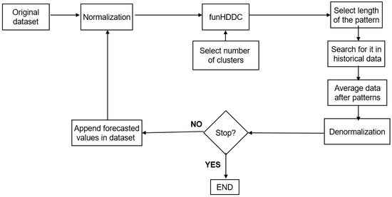
Figure 1.
Flowchart of the proposed algorithm.
Step 1: Data normalization. It is well known that data can range in large intervals for some variables. In order to minimize this effect, data are usually normalized. Although there are several strategies, the one selected for funPSF is the unity-based normalization, which brings all values into the range :
where denotes the normalized data, X the original data, the maximum value, and the minimum value.
Step 2: Selection of the optimal number of clusters, K. One of the main issues in clustering is the determination of the optimal number of partitions. There exist several indices; however, all of them search for optimality by optimizing different aspects [40]. For this reason, in this work, a majority voting system is used that combines the results of four well-known methods: silhouette [41], Dunn [42], Davies–Bouldin [43], and the Bayesian Information Criterion (BIC) [44]. Their application can lead to two situations: more than two indices (the majority) agree on choosing the same K (and then, this K is selected) or all four methods propose different K. When the second situation takes place, the second best values of the four indices are also considered (along with the first best values). The K selected is, then, the one pointed to by the majority of all the cases. Further, the best values can be analyzed until one K has more votes than the others.
Step 3: Application of the funHDDC functional clustering data algorithm. Let be an independent and identically distributed sample of multivariate curves, such that with . Under some regularity assumption, these multivariate curves can be represented as an infinite linear combination of orthogonal eigenfunctions: :
This decomposition is known as the Karhunen–Loeve expansion. It is worth noting that the computational cost of the Karhunen–Loeve transform is low as long as the observed curves are approximated in a finite basis function with a reasonable number of basis functions, which is the case in the present work.
In practice, the functional expressions of the observed curves are not known, and we only have access to discrete observations at a finite set of times. A common way to reconstruct the functional form of data is to assume that each curve can be approximated by a linear combination of basis functions (e.g., splines or Fourier): .
One consequence is that only a finite number of eigenfunctions can be computed in Equation (2), and the computational cost of the Karhunen–Loeve expansion computation is consequently low (more details in [6]).
funHDDC [7] is a model-based clustering algorithm for either univariate or multivariate functional data, which estimates for each curve the cluster to which it belongs. This algorithm relies on a Karhunen–Loeve decomposition per cluster, in order to propose a fine representation of the curves, and on the following distributional assumptions:
where .
Moreover, in order to provide a parsimonious modeling, a specific parametrization of the variance matrix is considered.
The inference of the model parameters is done through an EM algorithm:
- Initialization ;
- Repeat until convergence:
- (a)
- E step: compute ;
- (b)
- M step: update the model parameters as follows:
- with ;
- ;
- the elements are obtained from the diagonalization of where , and W contains the inner products between the basis function .
It is worth noting that the EM algorithm exhibits some convergence issues [45] that may lead to the failure of the whole procedure. However, these issues are not expected to occur with time series with daily or seasonal patterns, which is the usual situation in which funPSF can be successfully applied.
Figure 2 depicts an illustrative case, in which . It can be seen that once funHDDC is applied, the original time series is transformed into a sequence of labels: . Furthermore, for simplicity, it is considered that each pattern comprises one day (24 h), since it is a very common situation in problems in which funPSF can be efficiently applied.
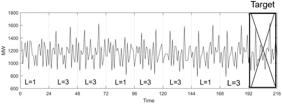
Figure 2.
Application of funHDDC to the time series and transformation into a sequence of labels.
Step 4: Selection of the length of the pattern sequence or window, W. The optimal number of labels forming W is determined by minimizing the forecasting error when funPSF is applied to a training set. In practice, W is calculated by means of cross-validation, whose validity to be used for evaluating time series prediction was recently discussed in [46]. The number of folds may vary according to the type of problem to be addressed. Figure 3 shows how W is determined when the training set is one year, and 12 folds are considered. It can be appreciated that the initial dataset is split into twelve folds (this number is used for simplicity and for a better physical understanding, since each fold represents one month). Then, every fold is used as test data, and the remaining eleven folds as training data. Errors for tests are reported when varying W from 1–10 and are denoted as . The average errors for are denoted as . Finally, the W that leads to minimal error is selected.
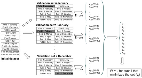
Figure 3.
Determining the length of the pattern sequence by means of cross-validation.
Step 5: Search for the pattern sequence within the historical data. At this stage of the algorithm, the dataset has already been discretized and the length of the pattern sequence determined. Hence, the sequence pattern, with length W, including the last (most recent) W labels, is retrieved, and the pattern sequence, , is created. is searched for within the historical data, and every time there is a match, the values identifying the next h are obtained.
Step 6: Generation of the forecast. Finally, all these values are averaged, weighting their contribution according to the distance to the present. That is, retrieved values closer to the target h have weights higher than those that occurred further into the past. Mathematically, it can be expressed as follows:
where is the forecasted sample, M is the number of matches encountered in the historical data, are the ith actual h values existing after a match, and the distance (or time elapsed) between the match and the h values that we want to predict.
Please note that Equation (3) does not use outputs’ feedback and this could limit the accuracy of the predictions, as discussed in [47]. However, original PSF and other published variants have shown prediction robustness despite this fact.
Figure 4 illustrates Steps 5 and 6. For this particular case, , and the pattern sequence . Two matches are depicted and the result of the weighted average for the values found just after the matches is the forecast itself.
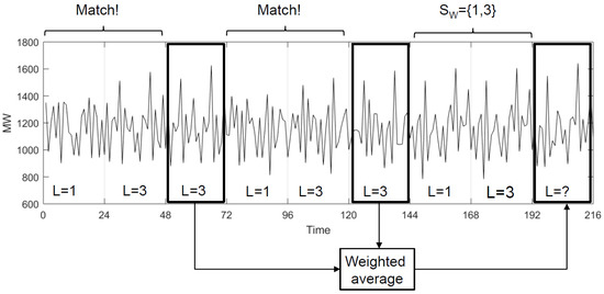
Figure 4.
Determining the length of the pattern sequence by means of cross-validation.
Step 7: Data denormalization. Once the forecast is done, this value must be denormalized, leading to the final forecast, . In this case, it consists of multiplying the forecast by the same value by which the data were normalized in Step 1:
Finally, Figure 5 shows the pseudocode for funPSF, where D denotes the dataset, K the number of clusters, L the labeled dataset such as , W the pattern sequence length or window, T the test set, and the forecasts for all data in T.
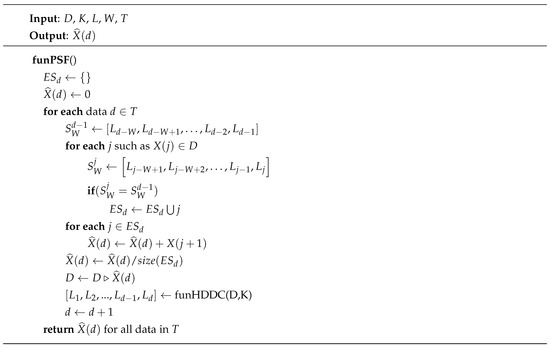
Figure 5.
A general scheme of the algorithm funPattern Sequence Forecasting (funPSF).
4. Results
The application of funPSF to real-world data is reported in this section. Section 4.1 describes the dataset used related to electricity demand from Uruguay. The quality measures to assess the funPSF performance are introduced in Section 4.2. Finally, the results achieved are shown and discussed in Section 4.4.
4.1. Data Description
This section describes the dataset that was used to evaluate the funPSF performance. It consists of data from 2007–2014 of electricity demand in Uruguay, retrieved on an hourly basis (70128 samples). The full dataset is available upon request from authors.
Data did not exhibit a significant number of outliers, since the application of the test proposed in [48] showed that less than 0.01% of the values were outliers. This fact led to the discarding of the use of methods particularly designed to deal with volatility or spike values.
In particular, the data distribution for different days of the week is represented, as well as the distribution for the full dataset is illustrated in Figure 6. Axis x for all subfigures denotes the amount of electricity in MW, while axis y denotes the accumulated frequency for such values. Differences in mean and skewness can be appreciated in different days of the week. In general, while working days were slightly left-skewed, it can be appreciated that weekends were slightly right-skewed, which means that lower consumption was reported on weekends, as expected. This fact justified generating, at least, different models for different types of days.
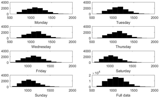
Figure 6.
Data distribution for days of the week, as well as for the full dataset.
4.2. Quality Measures
Given the nature of the data to be processed, three metrics were chosen to assess the performance of funPSF.
The first one was the mean absolute error (MAE), which is typically used in the electricity time series context. Operators are interested in the total amount of energy that must be generated, and that is the reason why they typically use absolute errors.
The second widely-used metric is the mean absolute percentage error (MAPE). This error provides information that is easier to interpret and compare.
Finally, the Root Mean Squared Error (RMSE) was also provided.
The associated formulas are:
where denotes the actual demand and the predicted demand for period h, and the bar above the squared differences is the mean.
4.3. Hardware and Software Resources
The experiments were carried out on the cluster physically located at the Data Science & Big Data Lab, Pablo de Olavide University. Each node forming the cluster shares the features listed in Table 1 and Table 2.

Table 1.
Features of the nodes: Hardware.
Table 2.
Features of the nodes: Software.
4.4. Performance Assessment
To assess the performance of funPSF, years 2013 and 2014 have been selected as test sets. The remaining years (2008–2012) have been used as training test sets. The standard 70–30% data division into training and test was applied. In particular, five out of seven years were used for training, which represents 71.43%. As shown in the original PSF paper, the algorithm needs no more than two years to find patterns in the historical data to perform accurate forecasts. As a consequence, it was determined that five years was a suitable choice.
Another relevant issue is the prediction horizon, h, which was set to one day given the typology of the problem, since the electricity industry typically plans the amount of energy that needs to be generated one day in advance.
In Section 4.1, it is shown that different days may have different data distributions. For this reason, while configuring the experimental setup, it was decided to use two strategies. First, funPSF was applied to the entire dataset, generating one single model regardless of the day of the week it had to be forecasted. Second, seven different models were generated, one per day, in order to better discover pattern sequences associated with different days of the week and festivities. It will be referred to as the 7-funPSF model in the rest of the paper.
The first parameter that must be calculated is the number of clusters that funHDDC must create, K. Values for K from 2–10 were considered in this study. The application of the majority voting system proposed in Section 3 yielded . Table 3 summarizes the results of all the indices individually proposed for the best and second best values. It can be seen that Dunn and BIC proposed as the best values, and Davies–Bouldin and silhouette proposed . Since no K had more votes than others, the second best values had to be observed. In this case, both Davies–Bouldin and silhouette also pointed to as the best election, whereas Dunn proposed and BIC . Therefore, since obtained four votes, it became the most voted K and was selected as the number of clusters to be created.
Table 3.
Determining the optimal number of clusters.
The second, and last, parameter required by funPSF is the length of the pattern sequence to be search for, W. Values for W from 2–10 were considered in this study. The cross-validation approach applied in the training set discovered that was the best value ( and ).
Moreover, ANN and ARIMA models have been applied. Both of them have been trained with the same training and test sets. The configuration found to be optimal was: (i) for ANN: 24 input neurons, one hidden layer, backpropagation, and the sigmoid activation function; (ii) .
Table 4 shows a performance summary for all four considered methods, and both MAE and MAPE errors. It can be seen that 7-funPSF clearly outperformed all of them. It can be seen that 7-funPSF obtained on average. This value represents a 28.07% improvement if compared to funPSF. Furthermore, the improvement reached 35.80% and 53.37% if compared to ANN and ARIMA, respectively. Analogously, 7-funPSF obtained the best MAPE: 5.63%. The relative reported improvements were 29.15%, 42.47%, and 58.00% when compared to funPSF, ANN, and ARIMA, respectively.
Table 4.
Summary of the achieved results in terms of mean absolute error (MAE) (MW), mean absolute percentage error (MAPE) (%), and Root Mean Squared Error (RMSE).
A thorough analysis of how MAE, MAPE, and RMSE behaved in all methods is reported in Table 5, Table 6, Table 7, Table 8, Table 9, Table 10, Table 11, Table 12 and Table 13. Table 5 shows how MAE was hourly distributed. It can be seen that 7-funPSF obtained lower errors for every hour, and overall, the error remained constant (except for Hours 19–21, where a moderate error increase can be seen). By contrast, ARIMA exhibited the worst behavior for 23 out of 24 h (all of them except for Hour 1). funPSF showed better performance than ANN in almost all the hours, except for Hours 8–13. However, ANN’s performance was very poor for the nighttime (Hours 1–6).
Table 5.
MAE summary for hours of the day.
Table 6.
MAE (MW) summary for months.
Table 7.
MAE (MW) summary for the type of day.
Table 8.
MAPE summary for the hour of the day (%).
Table 9.
MAPE summary for the month (%).
Table 10.
MAPE summary for the type of day (%).
Table 11.
RMSE summary for the hour of the day.
Table 12.
RMSE summary for the month.
Table 13.
RMSE summary for the type of day.
Another relevant piece of information that operators need to know is how algorithms behave in seasonal terms. For this reason, Table 6 shows how MAE was distributed over months. The behavior was similar for all studied methods. They reached the worst values for winter time (December and January) and for the beginning of the summer (June). 7-funPSF, again, obtained the best results for every month, whereas ARIMA obtained the worst results for all months. ANN slightly outperformed funPSF only in May (104.27 versus 106.77).
The third analysis carried out consisted of evaluating how the algorithms behaved for different day typologies. Specifically, Table 7 analyzes MAE values distinguishing between regular days and festivities. For regular days, MAE was almost constant for all methods. However, funPSF reported the worst value for Mondays. This fact is due to the search strategy followed, in which pattern sequences incorporate changes from weekends to working days. Fortunately, this effect is completely removed in 7-funPSF. By contrast, the situation for festivities was different. First, the reported errors were quite higher than those of regular days. Second, funPSF performed better than 7-funPSF. A possible justification is that with 7-funPSF, the size of training sets became smaller, and the forecasting of these few days should not be done by using this strategy. Overall, ANN and ARIMA kept reporting worse results than funPSF and 7-funPSF. Consequently, the development of new models for forecasting these particular days is suggested.
Similar conclusions can be drawn for MAPE, but with slight nuances. Table 8 reports the MAPE hourly distribution. 7-funPSF achieved the best results for all 24 h, with constant error. However, the behavior for ANN and ARIMA was quite different since their associated MAPE oscillated, combining small with high errors. Nevertheless, ARIMA reached the worst results for 21 out of 24 h, and ANN only slightly outperformed funPSF in four hours.
MAPE results in terms of months had no remarkable situations (see Table 9). 7-funPSF obtained the best results for all months; funPSF obtained the second best results for 11 out 12 months (December being the worst month, even worse than ANN and ARIMA); ARIMA reached the worst results for 11 out of 12 months; and ANN achieved results better than ARIMA, but worse than funPSF in 11 out of 12 months. Overall, funPSF, 7-funPSF, and ANN showed constant errors over time (no high fluctuations were reported throughout the different months).
MAPE differences between regular days and festivities are shown in Table 10. It is worth noting that 7-funPSF and funPSF obtained quite constant values for regular days and obtained the best and second best values for all considered measures. ANN and ARIMA showed higher fluctuations in their MAPE and reported the second worst and worst values for all days (except for two cases). As for festivities, again, funPSF showed better performance than the remaining methods, on average. It reached the best value in five out of seven days. 7-funPSF only obtained better results for two cases. ANN and ARIMA alternated between the worst and second worst results. Broadly speaking, the reported errors for festivities were quite larger than those of regular days, thus suggesting the development of particular models for these kinds of days.
Finally, Table 11, Table 12 and Table 13 report the accuracy in terms of RMSE. Almost the same conclusions can be drawn as those of MAPE, since both metrics are similar (except for the square root). Table 11 shows RMSE for every hour in the day. All methods exhibited two differentiated trends: from 4:00–21:00, RMSE was constantly increasing; however, from 21:00–4:00, errors decreased. There were no hours apparently in which the algorithms worked particularly well. Analogously, it seems that there were no hours in which the errors reached values that were particularly high. 7-funPSF obtained the best results in 21 out of 24 h. The remaining three best results were obtained by PSF (from 1:00–3:00). Neither ANN nor ARIMA reached the smallest error at any hour.
As for Table 12, it summarizes the estimated RMSE distributed over months. As expected, 7-funPSF obtained the best results for all twelve months. Only RMSE for May, November, and December exceeded 100, contrary to what the other methods reached: PSF only obtained RMSE less than 100 in three months, and ARIMA and ANN in two months. April and May were months that were particularly difficult to predict for ANN and ARIMA, with RMSE greater than 200. These values were quite unexpected, especially taking into account that the worst value for PSF was less than 150. Anyway, the behavior shown matched that of MAPE or MAE.
Table 13 summarizes RMSE disaggregated between regular days and festivities. It is especially remarkable that RMSE reached values that were extremely high for Tuesday and Wednesday when these days were festivities. This fact can be explained because they belong to central days of the week, and therefore, it is difficult to forecast such a pattern without external information. Overall, except for these two cases, the results were smooth, and no remarkable differences were reported between the best and worst values for all the methods.
Finally, a test of statistical significance was carried out. First, the D’Agostino–Pearson test [49] concluded that data obtained for this study did not meet the criteria of normality (). For this reason, a non-parametric test was selected to validate statistically the differences in the efficiency for all models. The non-parametric process followed was described in [50] and involved the use of the Friedman test. After executing the test, the obtained p-value was less than 0.0001. Therefore, the null hypothesis was rejected, and it can be concluded that the differences in the models were statistically significant.
5. Conclusions
A novel algorithm to forecast functional time series was proposed in this paper, as a result of the gap found after reviewing related literature. The main principle underlying the algorithm lies in the discovery of patterns within the historical data. To achieve such a goal, a functional clustering algorithm is first applied to the time series. This step results in transforming the time series into a sequence of labels, thus discretizing the original series. Later, a sequence of labels of arbitrary length, preceding the sample to be forecasted, is searched for. As the last step, the values occurring after matching the pattern sequence and the historical data are averaged, with weights associated with their distance. Real-world data related to electricity demand were used to assess the performance of the algorithm. Very promising results were reported and compared to other methods. It is also shown that the proposed approach obtained error values almost constant over time. The code is available for researchers in a ready-to-use R package (available upon acceptance). The main limitation of the proposed approach lies in its dependency on seasonal patterns within data: for chaotic time series or just for time series with no clear daily or seasonal patterns, funPSF might not work as desired. Alternatively, this method provides fast and accurate forecasts in the context of electricity demand. Future works are directed towards the development of novel funPSF models particularly adapted to dealing with anomalous data. The handling of multivariate functional time series is also a challenging task that will be addressed. In this sense, clustering algorithms to analyze multivariate data, as well as more suitable metrics must be used to fulfil such a task.
Author Contributions
Conceptualization, F.M.-Á. and J.J.; methodology, F.M.-Á. and J.J.; software, G.A.-C. and A.S.; writing, F.M.-Á. and J.J.; funding acquisition, F.M.-Á.
Funding
The authors would like to thank the Spanish Ministry of Economy and Competitiveness for the support under Projects TIN2014-55894-C2-R, P12-TIC-1728, and TIN2017-88209-C2-1-R. Francisco Martínez-Álvarez acknowledges support from José Castillejo Program CAS17/00379.
Acknowledgments
The authors also thank Prof. Jairo Cugliari for providing information about the datasets.
Conflicts of Interest
The authors declare no conflict of interest.
Abbreviations
| Algorithm | |
| PSF | Pattern Sequence Forecasting |
| funPSF | Functional Pattern Sequence Forecasting |
| ANN | Artificial Neural Networks |
| ARIMA | Autoregressive Integrated Moving Average |
| ARCH | Autoregressive Conditional Heteroskedasticity |
| ARMAX | Autoregressive Moving Average with Exogenous inputs model |
| EM | Expectation-Maximization |
| ANFIS | Adaptive Neuro-Fuzzy Inference System |
| Variables | |
| K | Number of clusters |
| W | Length of the window |
| D | Dataset |
| L | Labeled dataset |
| T | Test set |
| Pattern sequence | |
| M | Number of matches |
| h | Prediction horizon |
| Metrics | |
| MAE | Mean Absolute Error |
| MAPE | Mean Absolute Error |
| RMSE | Root Mean Squared Error |
References
- Ramsay, J.; Silverman, B.W. Functional Data Analysis; Springer: Berlin, Germany, 2005. [Google Scholar]
- Portela-González, J.; Munoz, A.; Alonso-Pérez, E. Forecasting Functional Time Series with a New Hilbertian ARMAX Model: Application to Electricity Price Forecasting. IEEE Trans. Power Syst. 2018, 33, 289–341. [Google Scholar]
- Horváth, L.; Kokoszk, P. Functional Time Series. Springer Ser. Stat. 2012, 200, 289–341. [Google Scholar]
- Martínez-Álvarez, F.; Troncoso, A.; Riquelme, J.C.; Aguilar-Ruiz, J.S. Energy time series forecasting based on pattern sequence similarity. IEEE Trans. Knowl. Data Eng. 2011, 23, 1230–1243. [Google Scholar] [CrossRef]
- Bokde, N.; Asencio-Cortés, G.; Martínez-Álvarez, F.; Kulat, K. PSF: Introduction to R Package for Pattern Sequence Based Forecasting Algorithm. R J. 2017, 9, 324–333. [Google Scholar]
- Bouveryon, C.; Jacques, J. Model-based Clustering of Time Series in Group-specific Functional Subspaces. Adv. Data Anal. Classi. 2011, 5, 281–300. [Google Scholar] [CrossRef]
- Schmutz, A.; Jacques, J.; Bouveyron, C.; Chèze, L.; Martin, P. Clustering Multivariate Functional Data in Group-Specific Functional Subspaces. 2017. Available online: https://hal.inria.fr/hal-01652467/ (accessed on 14 September 2018).
- Schmutz, A.; Jacques, J.; Bouveyron, C. funHDDC: Univariate and Multivariate Model-Based Clustering in Group-Specific Functional Subspaces; R package version 2.2.0, CRAN Reposity. Available online: https://rdrr.io/cran/funHDDC/ (accessed on 7 December 2018).
- Cincotti, S.; Gallo, G.; Ponta, L.; Raberto, M. Modelling and forecasting of electricity spot-prices: Computational intelligence vs. classical econometrics. AI Commun. 2014, 27, 301–314. [Google Scholar]
- Hyndman, R.J.; Shang, H.L. Forecasting functional time series. J. Korean Stat. Soc. 2009, 38, 199–211. [Google Scholar] [CrossRef]
- Lippi, M.; Bertini, M.; Frasconi, P. Short-Term Traffic Flow Forecasting: An Experimental Comparison of Time-Series Analysis and Supervised Learning. IEEE Trans. Intell. Transp. Syst. 2013, 14, 871–882. [Google Scholar] [CrossRef]
- Hormann, S.; Horvath, L.; Reeder, R. A functional version of ARCH model. Econ. Theory 2013, 29, 267–288. [Google Scholar] [CrossRef]
- Canale, A.; Vantini, S. Constrained functional time series: Applications to the Italian gas market. Int. J. Forecast. 2016, 32, 1340–1351. [Google Scholar] [CrossRef]
- Shang, H.L. Functional time series forecasting with dynamic updating: An application to intraday particulate matter concentration. Econ. Stat. 2017, 1, 184–200. [Google Scholar] [CrossRef]
- Kearney, F.; Cummins, M.; Murphy, F. Forecasting implied volatility in foreign exchange markets: A functional time series approach. Eur. J. Financ. 2017, 24, 1–14. [Google Scholar] [CrossRef]
- Yasmeen, F.; Hameed, S. Forecasting of Rainfall in Pakistan via Sliced Functional Times Series (SFTS). World Environ. 2018, 8, 1–14. [Google Scholar]
- Bebarta, D.K.; Bisoi, R.; Dash, P.K. Locally recurrent functional link fuzzy neural network and unscented H-infinity filter for short-term prediction of load time series in energy markets. In Proceedings of the IEEE International Conference on Systems, Man, and Cybernetics, Bhubaneswar, India, 15–17 October 2015; pp. 1394–1399. [Google Scholar]
- Qiu, X.; Suganthan, P.N.; Amaratunga, G.A.J. Electricity load demand time series forecasting with Empirical Mode Decomposition based Random Vector Functional Link network. In Proceedings of the IEEE International Conference on Systems, Man, and Cybernetics, Budapest, Hungary, 9–12 October 2016; pp. 1394–1399. [Google Scholar]
- Portela-González, J.; Munoz, A.; Sánchez-Úbeda, E.F.; García-González, J.; González, R. Residual demand curves for modeling the effect of complex offering conditions on day-ahead electricity markets. IEEE Trans. Power Syst. 2017, 32, 50–61. [Google Scholar] [CrossRef]
- Nhabangue, M.F.C.; Pillai, G.N.; Sharma, M.L. Chaotic time series prediction with functional link extreme learning ANFIS (FL-ELANFIS). In Proceedings of the IEEE International Conference on Power, Instrumentation, Control and Computing, Thrissur, India, 18–20 January 2018; pp. 1–6. [Google Scholar]
- Bokde, N.; Troncoso, A.; Asencio-Cortés, G.; Kulat, K.; Martínez-Álvarez, F. Pattern sequence similarity based techniques for wind speed forecasting. In Proceedings of the International work-conference on Time Series, Granada, Spain, 18–20 September 2017; pp. 786–794. [Google Scholar]
- Wang, Z.; Koprinska, I.; Rana, M. Pattern sequence-based energy demand forecast using photovoltaic energy records. In Proceedings of the International Conference on Artificial Neural Networks, Sardinia, Italy, 11–14 September 2017; pp. 486–494. [Google Scholar]
- Gupta, A.; Bokde, N.; Kulat, K.D. Hybrid Leakage Management for Water Network Using PSF Algorithm and Soft Computing Techniques. Water Resour. Manag. 2018, 32, 1133–1151. [Google Scholar] [CrossRef]
- Martínez-Álvarez, F.; Troncoso, A.; Riquelme, J.C.; Aguilar-Ruiz, J.S. Discovery of motifs to forecast outlier occurrence in time series. Pattern Recog. Lett. 2011, 32, 1652–1665. [Google Scholar] [CrossRef]
- Fujimoto, Y.; Hayashi, Y. Pattern sequence-based energy demand forecast using photovoltaic energy records. In Proceedings of the IEEE International Conference on Renewable Energy Research and Applications, Nagasaki, Japan, 11–14 November 2012; pp. 1–6. [Google Scholar]
- Koprinska, I.; Rana, M.; Troncoso, A.; Martínez-Álvarez, F. Combining pattern sequence similarity with neural networks for forecasting electricity demand time series. In Proceedings of the IEEE International Joint Conference on Neural Networks, Dallas, TX, USA, 4–9 August 2013; pp. 940–947. [Google Scholar]
- Shen, W.; Babushkin, V.; Aung, Z.; Woon, W.L. An ensemble model for day-ahead electricity demand time series forecasting. In Proceedings of the International Conference on Future Energy Systems, Berkeley, CA, USA, 21–24 May 2013; pp. 51–62. [Google Scholar]
- Jin, C.H.; Pok, G.; Park, H.W.; Ryu, K.H. Improved pattern sequence-based forecasting method for electricity load. IEEJ Trans. Electr. Electron. Eng. 2014, 9, 670–674. [Google Scholar] [CrossRef]
- Jacques, J.; Preda, C. Functional data clustering: A survey. Adv. Data Anal. Classif. 2014, 8, 231–255. [Google Scholar] [CrossRef]
- Yamamot, M. Clustering of functional data in a low-dimensional subspace. Adv. Data Anal. Classif. 2012, 6, 219–247. [Google Scholar] [CrossRef]
- Antoniadis, A.; Brossat, X.; Cugliari, J.; Poggi, J.M. Clustering Functional Data using Wavelet. Int. J. Wavel. Multiresolut. Inf. Process. 2013, 11. [Google Scholar] [CrossRef]
- Paparoditis, E.; Sapatinas, T. Short-term load forecasting: The similar shape functional time-series predictor. IEEE Trans. Power Syst. 2013, 28, 3818–3825. [Google Scholar] [CrossRef]
- Chaouch, M. Clustering-based improvement of nonparametric functional time series forecasting: Application to intra-day household-level load curves. IEEE Trans. Smart Grid 2014, 5, 411–419. [Google Scholar] [CrossRef]
- Antoniadis, A.; Brossat, X.; Cugliari, J.; Poggi, J.M. Clustering Functional Data on Convex Function Spaces. Methodol. Appl. Stat. Inference 2016, 16, 105–114. [Google Scholar]
- Kwon, A.; Ouyang, M. Clustering of Functional Data by Band Depth. In Proceedings of the International Conference on Bio-inspired Information and Communications Technologies, New York, NY, USA, 3–5 December 2016; pp. 510–515. [Google Scholar]
- Rivera-García, D.; García-Escudero, L.A.; Mayo, A.; Ortega, J. Robust Clustering for Time Series Using Spectral Densities and Functional Data Analysis. In Proceedings of the International Work-Conference on Artificial Neural Networks, Cadiz, Spain, 14–16 June 2017; pp. 142–154. [Google Scholar]
- Ieva, F.; Paganoni, A.M.; Tarabelloni, N. Covariance-based Clustering in Multivariate and Functional Data Analysis. J. Mach. Learn. Res. 2016, 17, 1–21. [Google Scholar]
- Park, J.; Ahn, J. Clustering multivariate functional data with phase variation. Biometrics 2017, 73, 324–333. [Google Scholar] [CrossRef] [PubMed]
- Tokushige, S.; Yadohisa, H.; Inada, K. Crisp and fuzzy k-means clustering algorithms for multivariate functional data. Comput. Stat. 2017, 22, 1–16. [Google Scholar] [CrossRef]
- Sabo, K.; Scitovski, R. An approach to cluster separability in a partition. Inf. Sci. 2015, 305, 208–218. [Google Scholar] [CrossRef]
- Kaufman, L.; Rousseeuw, P.J. Finding Groups in Data: An Introduction to Cluster Analysis; Wiley: Hoboken, NJ, USA, 1990. [Google Scholar]
- Dunn, J. Well separated clusters and optimal fuzzy partitions. J. Cybern. 1974, 4, 95–104. [Google Scholar] [CrossRef]
- Davies, D.L.; Bouldin, D.W. A cluster separation measure. IEEE Trans. Pattern Anal. Mach. Intell. 2000, 1, 224–227. [Google Scholar] [CrossRef]
- Schwarz, G.E. Estimating the dimension of a model. Ann. Stat. 1978, 6, 461–464. [Google Scholar] [CrossRef]
- Wu, C.F.J. On the convergence properties of the EM algorithm. Ann. Stat. 1983, 11, 95–103. [Google Scholar] [CrossRef]
- Bergmeir, C.; Hyndman, R.J.; Koo, B. A note on the validity of cross-validation for evaluatingautoregressive time series prediction. Comput. Stat. Data Anal. 2018, 120, 70–88. [Google Scholar] [CrossRef]
- Capizzi, G.; Lo-Sciuto, G.; Napoli, C.; Tramontana, E. Advanced and Adaptive Dispatch for Smart Grids by Means of Predictive Models. IEEE Trans. Smart Grid 2017, 6, 6684–6691. [Google Scholar] [CrossRef]
- Gelper, S.; Fried, R.; Croux, C. Robust forecasting with exponential and Holt-Winters smoothing. J. Forecast. 2010, 29, 285–300. [Google Scholar]
- D’Agostino, R.B.; Belanger, A.; D’Agostino, R.B., Jr. A suggestion for using powerful and informative tests of normality. Am. Stat. 1990, 44, 316–321. [Google Scholar]
- García, S.; Herrera, F. An extension on statistical comparisons of classifiers over multiple data sets for all pairwise comparisons. J. Mach. Learn. Res. 2008, 9, 2677–2694. [Google Scholar]
© 2018 by the authors. Licensee MDPI, Basel, Switzerland. This article is an open access article distributed under the terms and conditions of the Creative Commons Attribution (CC BY) license (http://creativecommons.org/licenses/by/4.0/).