Abstract
In this paper, a fault-tolerant control method is proposed for quadcopter unmanned aerial vehicles (UAV) to account for system uncertainties and actuator faults. A mathematical model of the quadcopter UAV is first introduced when faults occur in actuators. A normal adaptive sliding mode control (NASMC) approach is proposed as a baseline controller to handle the chattering problem and system uncertainties, which does not require information of the upper bound. To improve the performance of the NASMC scheme, radial basis function neural networks are combined with an adaptive scheme to make a quick compensation in presence of system uncertainties and actuator faults. The Lyapunov theory is applied to verify the stability of the proposed methods. The effectiveness of modified ASMC algorithm is compared with that of NASMC using numerical examples under different faulty conditions.
1. Introduction
Quadcopter unmanned aerial vehicles (UAVs) are used in a wide range of applications and research, oweing to their various benefits include agility, economical cost, small size, mechanical simplicity, and ability to operate in dangerous environments, which has led them to be more popular than other UAV systems. Therefore, they have been studied and tested in various technologies including target tracking [1,2], fault diagnosis, and fault tolerant control [3,4,5], and formation control [6,7].
In real applications, the translation movement of the quadcopter is controlled by an operator with the support of a remote-control system, whereas rotation movement is operated automatically via an onboard controller unit. To operate a quadcopter in the desired position the attitude controller plays an important role, because it allows the quadcopter to maintain the desired rotation and prevents crashing when the operator performs the desired translation movement [8]. One problem with the attitude control of quadcopter UAVs is the uncertainties and unknown disturbances that the quadcopter is subjected to during operation. This issue has been investigated previously based on various control methods, such as adaptive control [9], sliding mode control [10,11], and backstepping control [12,13]. If faults occur, control of the quadcopter becomes more challenging [14], which could result in a failure during the mission. Therefore, fault-tolerant control (FTC) is a key factor that needs be considered intensively in attitude-controller design. The topic of FTC has drawn attention in academic communities owning to enhanced safety and reliability demands. In general, there are three type of faults in FTC systems: Actuator, sensor, and process faults. Since the actuator is an important component that can connect control signals and specific movements to achieve a particular objective, actuator faults are addressed in this article. Passive FTC methods are used to accommodate this type of fault, which do not require fault detection and identification units as in active FTC methods [13]. Actuator faults are examined as uncertainties and they are treated using the passive FTC approach. Sliding mode control (SMC) is a passive FTC method for designing control systems dealing with model uncertainties and external disturbances. Studies by Kacimi et al. [13], Sharifi et al. [14], and Bouchoucha et al. [15] show some acceptable results using SMC approaches. SMC has the advantage of insensitivity to unknown disturbances and parametric uncertainties which makes it a promising method [16]. However, the bound of uncertainties needs to be designed in traditional SMCs. In several applications, the magnitude of the actuator fault cannot be known, and it is difficult to achieve the bound of uncertainty in advance. This motivates a new control method, which combines adaptive algorithms with SMC to enhance the tracking performance and robustness of the system without knowledge of the information of the uncertainty bound. Many existing studies have introduced the design of adaptive SMC [17,18,19,20,21,22,23], which integrates the adaptive law into the normal SMC to enhance the robustness of control performance. However, these studies have not investigated the actuator faults in the quadcopter model.
There are minor studies using adaptive SMC approaches to handle actuator faults. In references [24,25,26], the ASMC shows good results for the tracking performance with an actuator fault; however, these control approaches may not have sufficient robustness because the accurate model needs to be achieved in state space representation. Another complex method based on a fuzzy system is proposed in reference [27]. A fuzzy compensator is used to handle disturbances, actuator faults, and to avoid the high gain of adaption rate but this control law still requires the information of bound and it is challenging to find the fuzzy rule through the trial and error method. The active FTC based on adaptive SMC approach have been proposed in reference [28]. The results show good tracking performance in presence of actuator faults but the fault identification unit is required in this approach. Moreover, adaptive SMC based on the neural network have been investigated in reference [29,30,31]. These approaches show good responses without accurate model but actuator faults are not considered. The most recent work [10] proposed a simple adaptive SMC to handle uncertainties and disturbances. This method is simple to implement on quadcopter design and it shows good tracking performance. However, when a large fault occurs, this method cannot compensate quickly because the adaption rate is limited to ensure system stability. To solve this problem, radial basis function (RBF) neural networks are integrated into adaptive SMC [10] for fault identification and reconstruction through on-line approximation technique, which motivates our work in this paper.
In this article, we concentrate on developing an FTC method that can handle system uncertainties and actuator faults. The proposed method has some advantages such as using structure of RBF neural networks for fault identification and reconstruction, and using a simple adaptive scheme to avoid system uncertainties, and the chattering phenomenon. Moreover, this approach does not require the bound of uncertainty and fault detection unit which is different than the method in reference [32]. Finally, the control scheme in this paper is suitable for flight systems where the attitude control operates at a higher frequency than position control, which is different to the previous paper [33]. Unlike the paper [33], the radial basis function neural networks in this work are simpler than the fuzzy approach for fault reconstruction because the limitation of the fuzzy method is a trial and error technique for adjusting input variables. The contributions of this article can be summarized as follows. First, a mathematical model of the quadcopter is introduced with parametric uncertainties and disturbances. Second, a proportional-integral-derivative (PID) controller is used as position controller. Third, the RBF neural network scheme is proposed for fault identification and accommodation, whereas the adaptive scheme is used to handle the chattering phenomenon and uncertainties of system dynamics. Finally, the stability of the system is verified using the Lyapunov theory.
2. Quadcopter Modeling
2.1. Modeling of Quadcopter in Healthy Operation
The dynamics of the quadcopter UAV using Euler-Lagrange equations is described by Main and Daobo [20]. Figure 1 shows the torques and forces acting on the quadcopter. Assume that the dynamics of the quadcopter are considered in body-fixed coordinate B and earth-fixed coordinate E. The front and rear (1 and 3) motors rotate in a counter-clockwise direction; the other motors (2 and 4) rotate in a clockwise direction. The distance from the center to each rotor is denoted by .
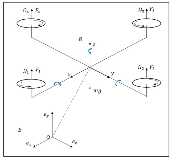
Figure 1.
Quadcopter configuration.
The rotational and translation movement of the quadcopter can be described as follows [5,10]:
where represent the moments of inertia along the directions, respectively; and are drag coefficients which depend on flight conditions; is the moment of inertia of each motor, and ; is the total mass; and denote the Euler angles; and represent the position of the quadcopter; and the four control inputs can be presented as
where and represents the torque and thrust force produced by the motor; are positive constants depending on the density of air, the radius of propeller, number of blades and geometry [11]; represents the rotational speed of the motor. is the total thrust; are the torques in the directions, which correspond to the roll, pitch, and yaw Euler angles, respectively.
2.2. Modeling of Quadcopter in Faulty Operation
The dynamic model of the quadcopter in faulty operation can be presented by
where and are control inputs in faulty operation described by
The fault model of the actuator can be presented by
where indicates that the actuator loses partial effectiveness; the actuator is in healthy operation when ; the actuator loses effectiveness completely when .
Substituting Equation (4) into Equation (3), we achieve
where the unknown terms are presented by
3. Controller Design
The control strategy of the quadcopter is presented in Figure 2. The altitude of the quadcopter is controlled by the total thrust (). The desired angles of roll () and pitch () are used for the rotational controller, which is achieved through the position controller. The desired yaw () is used to control the heading through the yaw controller (heading controller). The actual positions and are achieved from the GPS unit, which is converted from the latitude and longitude signals. The actual angles and are measured from the inertial measurement unit. The control inputs and are used to control the rotation movement of the quadcopter.
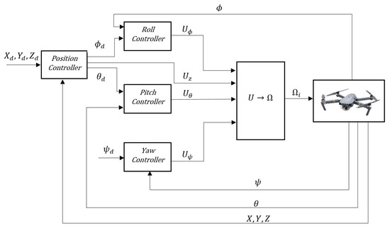
Figure 2.
Control scheme of the quadcopter.
3.1. Fault Tolerant Control for Attitude System Using Normal Adaptive Sliding Mode Approach
Define the state vector and control inputs . Then, the rotational movement equations of the quadcopter have the following form:
Roll control system
where , , ; is the system uncertainty.
Pitch control system
where , , ; is the system uncertainty.
Yaw control system
where , , ; is the system uncertainty.
Based on these rotational movement equations, each subsystem can be derived in the following form:
Let us define the desired attitude . The control objective is to find the control law such that the quadcopter can track the desired attitude , i.e., as , .
Define the control error:
The sliding surface equation can be expressed as
where is the positive gain.
The derivative of the sliding surface can be described as
From Equations (12) and (14), can be described as
With the sliding surface in Equation (14), the fault tolerant control law can be expressed as
and updated by [10]
where and are positive numbers, and denotes the sign function.
Theorem 1.
If the sliding surface and control law are designed as Equations (14) and (16), then the nonlinear system Equation (11) is stable and the control errors are forced to zero.
Proof.
Choose the Lyapunov function as follows
where ; is the estimate of ; .
Take the first derivative of the Lyapunov function
Substituting Equations (16) and (17) into Equation (19), we obtain
□
Assumption 1.
The uncertaintyand the resultant of actuator faultsare supposed to be bounded byand, whereandare unknown positive constants. There exists the unknown parametersuch that.
From Assumption 1, it is shown that . Assuming that , from Equation (14), we can obtain
Because is a positive number, Equation (14) can be expressed as
Remark 1.
Equation (22) shows that the NASMC designed as Equation (14) guarantees Lyapunov stability of system Equation (12). If, then the control errors are forced to zero, which ensures the stability of the closed-loop system.
Remark 2.
To avoid the chattering phenomenon due to sign function in control law Equation (16), a saturation function is introduced as
Remark 3.
In this method, only one parameter is designed to handle both system uncertainties and actuator faults. In Section 3.2, an RBF network is combined with adaptive law to handle system uncertainties and the actuator fault separately to ensure a quicker response during actuator faults.
3.2. Fault Tolerant Control for Attitude System Using Modified Adaptive Sliding Mode Approach
In this section, an RBF neural network is used to approximate function to handle the actuator fault while the adaptive law is used to handle chattering and system uncertainties. The approximation method using the RBF network is presented in reference [34] as follows:
where is the input of the RBF neural network; the number of hidden nodes, is the output of Gaussian function, is the approximation weight, is the approximation error assumed to be bounded by , in which is a small positive constant.
The structure of the RBF network is shown in Figure 3. It consists of three layers: One input layer, one hidden layer, and one output layer. The inputs of the network are and .
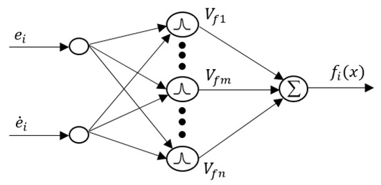
Figure 3.
Structure of radial basis function (RBF) neural network.
Assumption 2.
There exists an unknown parametersuch that
Theorem 2.
Consider the actuator fault in the system Equation (6) and the sliding surface in Equation (13). Suppose that the modified adaptive sliding mode control (MASMC) scheme for fault tolerant control is proposed as
and updated by
whereare positive gains. Then, it ensures that the stability of the closed-loop system and the control errors are forced to zero.
Proof.
Lyapunov function candidate is chosen as follows
where ; are the estimates of and , respectively.
Taking the first derivative of Lyapunov function candidate Equation (29), we obtain
From Assumption 2, it shows that . Because is a positive number, we obtain
□
3.3. Position Control
A PID controller is applied to control the translational movements of the quadcopter as follows
where , and are the desired positions in the and directions, respectively; and are actual values; and and are the controller gains.
Assume that the vehicle does not pass through singularities (). From translational movement Equation (1), we obtain the desired roll, pitch, and total thrust:
4. Simulation and Evaluation
In this section, to show the effectiveness of the proposed method, the quadcopter parameter in reference [10] is used for the simulation. The motion of the quadcopter is examined to track the desired roll angle with an actuator fault. The quadcopter is assumed to hover in position-hold mode. A filter is applied to generate the desired roll angles as follows [26]
where starts at and increases to at 5 s, and decrease to at 10 s; then, it changes from to at 15 s, and increases to at 20 s, finally, remains at for the remaining time. Four different actuator faults are presented. The first case considers the 10% loss of control effectiveness (LoCE) in actuator 2 at 14s. In the second situation, the 50% LoCE in actuator 2 at 14 s and 20% uncertainty of inertia are examined. In the third case, the quadcopter is commanded to track the desired trajectory with 50% LoCE in both actuator 2 and 3 at 50 s and 70 s. In the final case, the quadcopter is commanded to track the desired trajectory with 50% LoCE in both actuator 1 and 3 at 50 s and 70 s.
For NASMC, parameters were selected as , and . For comparison, the same parameters of were chosen in the proposed MASMC, and the remaining parameter was selected as 50. In position controller, were chosen.
4.1. Case 1: 10% LoCE in Actuator 2
Figure 4 compares the tracking performance of the roll angle and error between the NASMC and MASMC methods, with 10% LoCE in actuator 2. From the initial time to 14 s, both methods can make a good tracking in roll angle and error with the same control input value shown in Figure 5a. In this stage, the control input is increased abruptly to change the roll angle from to at 5 s, and then it is decreased to change the roll angle from to at 10 s. After a small magnitude of fault is injected into actuator 2 at 14 s, the MASMC compensates quickly to track the desired roll angle. Furthermore, the MASMC demonstrates a quicker tracking error than the ASMC owning to it greater control effort when a fault occurs. From 15 s to 30 s, there is a similar trend in control effort for both NASMC and MASMC, which decreases the control effort at 15 s in order to change the roll angle from to , and then increases the control effort at 20 s to change roll angle from to . It should be noted that after fault occurs the MASMC can converge quickly to zero in tracking error. In all figures, and represent the desired roll angle, actual roll angle using MASMC, and the actual roll angle using NASMC, respectively. and represent the errors in roll angle using MASMC and NASMC. and are the moments of roll determined from MASMC and NASMC through Equation (2).
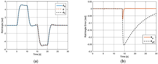
Figure 4.
Comparison of tracking performance between normal adaptive sliding mode control (NASMC) and modified adaptive sliding mode control (MASMC) with 10% loss of control effectiveness (LoCE) in actuator 2: (a) Roll angle; (b) tracking error.
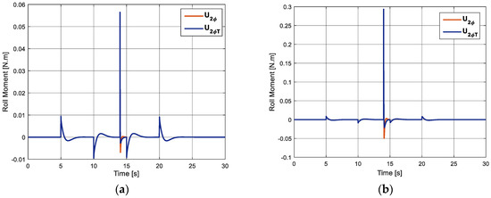
Figure 5.
Comparison of Control torque between NASMC and MASMC: (a) 10% LoCE in actuator 2; (b) 50% LoCE in actuator 2.
4.2. Case 2: 50% LoCE in Actuator 2 and 20% Uncertainties of the Inertia
To demonstrate the effectiveness of MASMC, a large fault is injected into actuator 2 with 50% LoCE at 14 s and 20% uncertainties of inertia is examined in the model of a quadcopter. Similar to case 1, from the initial time to 14 s, Figure 5b and Figure 6 show that both methods can use the same control torque value and make a good tracking in roll angle and error. When actuator fault is increased to 50% LoCE at 14 s, the NASMC shows an oscillation response at the initial stage and a low compensation to track the desired roll angle. In contrast, MASMC presents a very good tracking performance although there is a small overshoot at the initial stage after fault occurs. MASMC uses more control effort than ASMC when a fault occurs, and after 15 s there is a similar control effort for both NASMC and MASMC. It should be noted that after 15 s, there is a slow response in tracking performance of NASMC compared with MASMC shown in Figure 6.
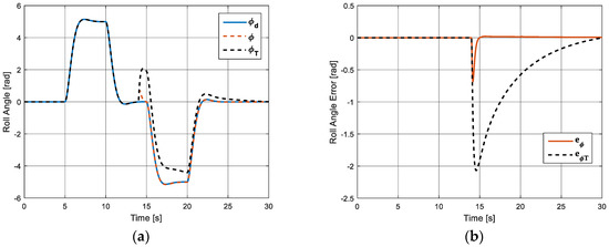
Figure 6.
Comparison of tracking performance between NASMC and MASMC with 50% LoCE in actuator 2: (a) Roll angle; (b) tracking error.
In both cases, by integrating the RBF neural networks into the NASMC approach the tracking error in roll angle can converge quickly to zero after fault occurs. The MASMC in both cases can detect and accommodate faults automatically through on-line approximation without using the fault detection unit.
4.3. Case 3: Multiple Faults Occuring in Actuator 2 and 3
This section shows the performance of MASMC in the presence of multiple faults occurring in actuator 2 and 3. Figure 7 presents the tracking performance in three positions while Figure 8, Figure 9 and Figure 10 show the corresponding Euler angles , sliding surface, and control inputs . According to these figures, when faults occur in actuator 2 and 3 at 50 s and 70 s, respectively, the altitude is decreased at 50 s and 70 s due to loss of thrust force, and then it can compensate steadily through the PID controller. The actual trajectories in directions can converge quickly to the desired ones in the presence of faults. It should be noted that when the attitude controller can respond quickly to handle actuator faults through the fault tolerant controller, the responses of x, y directions will be improved.
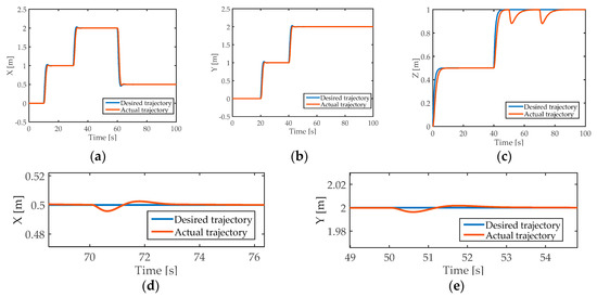
Figure 7.
Tracking performance in three positions: (a) x-direction; (b) y-direction; (c) z-direction; (d) zoomed x-direction at 50 s; (e) zoomed y-direction at 70 s.
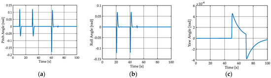
Figure 8.
Tracking performance of Euler angles: (a) Pitch angle; (b) roll angle; (c) yaw angle.
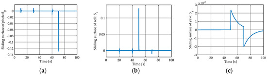
Figure 9.
Sliding surface: (a) Pitch angle; (b) roll angle; (c) yaw angle.
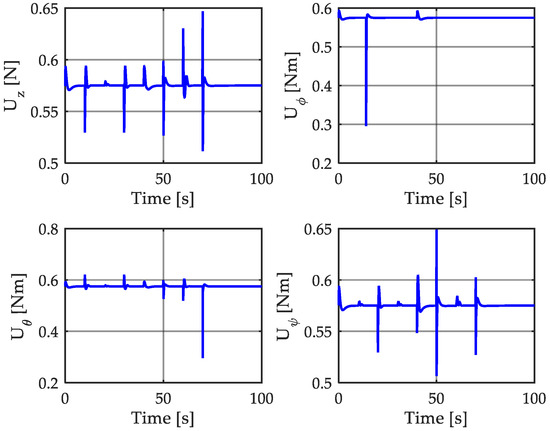
Figure 10.
Control inputs.
4.4. Case 4: Multiple Faults Occuring in 1 and 3
In this situation, 50% LoCE in actuator 1 and 3 is considered at 50 s, and 70 s, respectively. Figure 11 presents the tracking performance in three positions while Figure 12, Figure 13 and Figure 14 show the corresponding Euler angles , sliding surface, and control inputs . According these figures, when faults occur at 50 s and 70 s, the altitude is decreased at 50 s and 70 s due to loss of thrust force and then altitude can compensate steadily through the PID controller. The actual trajectories in directions can converge quickly to the desired ones in the presence of faults. It should be noted that although faults occur on the same axis of the quadcopter, the system still maintains the stability.
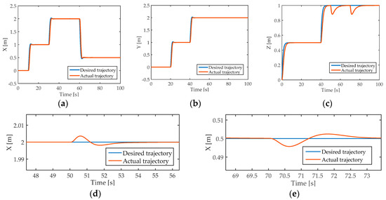
Figure 11.
Tracking performance in three positions: (a) x-direction; (b) y-direction; (c) z-direction; (d) zoomed x-direction at 50 s; (e) zoomed x-direction at 70 s.
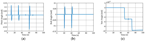
Figure 12.
Tracking performance of Euler angles: (a) Pitch angle; (b) roll angle; (c) yaw angle.
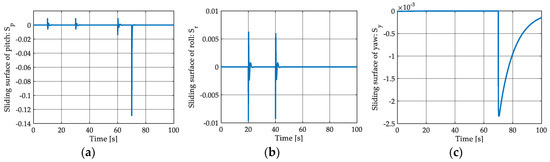
Figure 13.
Sliding surface: (a) Pitch angle; (b) roll angle; (c) yaw angle.
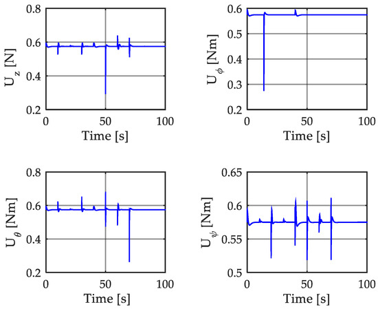
Figure 14.
Control inputs.
Remark 4.
In all cases, the computational complexity in MASMC depend on hidden nodes in RBF neural networks. Therefore, the user can choose the suitable hidden nodes for controller design. For simplicity, we used seven hidden nodes in MASMC.
5. Conclusions
In this paper, a model of a quadcopter was examined in the presence of actuator faults and uncertainties. An NASMC was designed as a baseline controller to handle actuator faults, uncertainties, and chattering phenomenon. An MASMC which integrates RBF neural network into NASMC was investigated to make a quick compensation when large faults occur. The proposed MASMC does not require a fault identification unit and bound of uncertainty. To verify the suggested method, the model of the quadcopter along with the proposed controllers were simulated in different cases. The results show that the MASMC can make a quick compensation and a good trajectory tracking compared with NASMC. However, the limitation of this work is that the proposed MASMC does not consider the complete loss of the actuator fault and does not verify through experiment. The future research should concentrate on experimental results of the proposed method, and should examine complete loss effectiveness in actuator using the fault identification technique.
Author Contributions
Conceptualization, N.P.N. and S.K.H.; methodology, N.P.N.; software, N.P.N.; validation, N.P.N.; formal analysis, N.P.N.; investigation, N.P.N.; resources, N.P.N.; data curation, N.P.N.; writing—original draft preparation, N.P.N.; writing—review and editing, S.K.H.; visualization, N.P.N.; supervision, S.K.H.; project administration, S.K.H.; funding acquisition, S.K.H.
Funding
This research received no external funding.
Acknowledgments
This research was supported by the MSIT (Ministry of Science and ICT), Korea, under the ITRC (Information Technology Research Center) support program (IITP-2018-2018-0-01423) supervised by the IITP (Institute for Information & communications Technology Promotion). The authors gratefully acknowledge the helpful comments and suggestions of the reviewers which have improved the presentation.
Conflicts of Interest
The authors declare no conflict of interest.
References
- Ren, W.; Beard, R.W. Trajectory tracking for unmanned air vehicles with velocity and heading rate constraints. IEEE Trans. Control Syst. Technol. 2004, 12, 706–716. [Google Scholar] [CrossRef]
- Bonna, R.; Camino, J.F. Trajectory Tracking Control of a Quadcopter Using Feedback Linearization. In Proceedings of the XVII International Symposium on Dynamic Problems of Mechanics, Natal-Rio Grande Do Norte, Brazil, 22–27 February 2015. [Google Scholar]
- Nguyen, N.P.; Hong, S.K. Robust Fault Diagnosis for a Quadrotor with Actuator Fault. I. J. Engineer. Technol. 2018, 7, 74–77. [Google Scholar] [CrossRef]
- Chen, F.; Lei, W.; Tao, G.; Jiang, B. Actuator Fault Estimation and Reconfiguration Control for Quad-rotor Helicopter. Int. J. Adv. Robot. Syst. 2016, 13. [Google Scholar] [CrossRef]
- Nguyen, N.P.; Hong, S.K. Sliding mode Thau observer for actuator fault diagnosis of quadcopter UAVs. Appl. Sci. 2018, 8, 1893. [Google Scholar] [CrossRef]
- Zhao, W.; Go, T.H. Quadcopter formation flight control combining MPC and robust feedback linearization. J. Frankl. Inst. 2014, 351, 1335–1355. [Google Scholar] [CrossRef]
- Mahmood, A.; Kim, Y. Decentralized formation flight control of quadcopters using robust feedback linearization. J. Frankl. Inst. 2017, 354, 852–871. [Google Scholar] [CrossRef]
- Tayebi, A.; McGilvray, S. Attitude stabilization of VTOL quadrotor aircraft. IEEE Trans. Control Syst. Technol. 2006, 14, 562–571. [Google Scholar] [CrossRef]
- Dydek, Z.T.; Annaswamy, A.M.; Laveretsky, E. Adaptive control of quadrotor UAVs: A design trade study with flight evaluation. IEEE Trans. Control Fault Toler. Syst. 2012, 21, 1400–1406. [Google Scholar] [CrossRef]
- Nadda, S.; Swarup, A. On adaptive sliding mode control for improved quadrotor tracking. J. Vib. Control 2017, 24, 3219–3230. [Google Scholar] [CrossRef]
- Zheng, E.H.; Xiong, J.J.; Luo, J.L. Second order sliding mode control for quadrotor UAV. ISA Trans. 2014, 53, 1350–1356. [Google Scholar] [CrossRef]
- Bouabdallah, S.; Siegwart, R. Backstepping and Sliding mode techniques applied to an indoor micro quadrotor. In Proceedings of the IEEE International Conference on Robotics and Automation, Barcelona, Spain, 18–22 April 2005; pp. 2247–2252. [Google Scholar]
- Kacimi, A.; Mokhtari, A.; Kouadri, B. Sliding mode control based on adaptive backstepping approach for quadrotor unmanned aerial vehicle. Prz. Elektrotech. 2012, 88, 188–193. [Google Scholar]
- Sharifi, F.; Mirzaei, M.; Gordon, B.W.; Zhang, Y.M. Fault tolerant control of a quadrotor UAV using sliding mode control. In Proceedings of the Conference on Control and Fault Tolerant Systems, Nice, France, 6–7 October 2010; pp. 239–244. [Google Scholar]
- Bouchoucha, M.; Seghour, S.; Tadjine, M. Classical and second order sliding mode control solution to an attitude stabilization of a four rotors helicopter: From theory to experiment. In Proceedings of the 2011 IEEE International Conference on Mechatronics, Istanbul, Turkey, 13–15 April 2011. [Google Scholar]
- Barghandan, S.; Badamchizadeh, M.A.; Jahed-Motlagh, M.R. Improve Adaptive Fuzzy Sliding Mode Controller for Robust Fault Tolerant of a Quadrotor. Int. J. Control Autom. Syst. 2017, 15, 427–441. [Google Scholar] [CrossRef]
- Yang, H.; Jiang, B.; Zhang, K. Direct self-repairing control of the quadrotor helicopter based on adaptive sliding mode control technique. In Proceedings of the 2014 IEEE Chinese Guidance, Navigation and Control Conf, Yantai, China, 8–10 August 2014. [Google Scholar]
- Nicol, C.; Macnab, C.J.B.; Ramirez-Serrano, A. Robust neural network control of a quadrotor helicopter. In Proceedings of the Canadian Conference on Electrical and Computer Engineering, Niagara Falls, ON, Canada, 4–7 May 2008. [Google Scholar]
- Dierks, T.; Jagannathan, S. Output feedback control of a quadrotor UAV using neural networks. IEEE Trans. Neural Netw. 2010, 21, 50–66. [Google Scholar] [CrossRef] [PubMed]
- Boudjedir, H.; Yacef, F.; Bouhali, O.; Rizoug, N. Adaptive neural network for a quadrotor unmanned aerial vehicle. Int. J. Found. Comput. Sci. Technol. 2012, 2, 1–13. [Google Scholar] [CrossRef]
- Karimi, H.; Chadli, M.; Shi, P. Fault detection, isolation, and tolerant control of vehicles using soft computing methods. IET Control Theory Appl. 2014, 8, 655–657. [Google Scholar] [CrossRef]
- Akhenak, A.; Chadli, M.; Maquin, D.; Ragot, J. Design of a sliding mode fuzzy observer for uncertain Takagi-Sugeno fuzzy model: Application to automatic steering of vehicles. Int. J. Veh. Auton. Syst. 2007, 5, 288–305. [Google Scholar] [CrossRef]
- Dahmani, H.; Chadli, M.; Rabhi, A.; El Hajjaji, A. Road curvature estimation for vehicle lane departure detection using a robust Takagi–Sugeno fuzzy observer. Veh. Syst. Dyn. 2013, 51, 581–599. [Google Scholar] [CrossRef]
- Hu, Q.; Xiao, B. Adaptive fault tolerant control using integral sliding mode strategy with application to flexible spacescraft. Int. J. Syst. Sci. 2013, 44, 2273–2286. [Google Scholar] [CrossRef]
- He, J.; Qi, R.; Jiang, B.; Qian, J. Adaptive output feedback fault tolerant control design for hypersonic flight vehicles. J. Frankl. Inst. 2015, 352, 1811–1835. [Google Scholar] [CrossRef]
- Wang, B.; Zhang, Y.M. Adaptive sliding mode fault-tolerant control for an unmanned aerial vehicle. Unmanned Systems. World Sci. 2017, 5, 209–221. [Google Scholar] [CrossRef]
- Mian, A.A.; Daobo, W. Modeling and backstepping based nonlinear control strategy for a 6 DOF quadrotor helicopter. Chin. J. Aeronaut. 2008, 21, 261–268. [Google Scholar] [CrossRef]
- Abdel-Razzak, M.; Hassan, N.; Francois, B. Active fault tolerant control of quadrotor UAV Using Sliding mode control. In Proceedings of the International Conference on Unmanned Aircraft Systems, Orlando, FL, USA, 27–30 May 2014. [Google Scholar]
- Kim, B.S.; Calise, A.J. Nonlinear flight control using neural networks. AIAA J. Guid. Control Dyn. 1997, 20, 26–33. [Google Scholar] [CrossRef]
- Fei, J.; Ding, H. Adaptive sliding mode control of dynamic systems using RBF neural network. Nonlinear Dyn. 2012, 70, 1563–1573. [Google Scholar] [CrossRef]
- Fei, J.; Lu, C. Adaptive sliding mode control of a dynamics systems using double loop recurrent neural network structure. IEEE Trans. Neural Netw. Learn. Syst. 2018, 29, 1275–1286. [Google Scholar] [CrossRef]
- Akhenak, A.; Chadli, M.; Maquin, D.; Ragot, J. Sliding mode multiple observer for fault detection and isolation. In Proceedings of the 42nd IEEE Conference on Decision and Control, Maui, HI, USA, 9–12 December 2003. [Google Scholar]
- Bououden, S.; Chadli, M.; Karimi, H.R. Fuzzy sliding mode controller design using Takagi-Sugeno modelled nonlinear systems. Math. Probl. Eng. 2013, 2013, 734094. [Google Scholar] [CrossRef]
- Wang, Z.; Shen, Y.; Zhang, X. Actuator fault estimation for a class of nonlinear descriptor systems. Int. J. Syst. Sci. 2014, 45, 487–496. [Google Scholar] [CrossRef]
© 2018 by the authors. Licensee MDPI, Basel, Switzerland. This article is an open access article distributed under the terms and conditions of the Creative Commons Attribution (CC BY) license (http://creativecommons.org/licenses/by/4.0/).