Dynamic Placement Analysis of Wind Power Generation Units in Distribution Power Systems

Abstract

The placement problem of distributed generators (DGs) in distribution networks becomes much more complicated in the case of using the DGs with renewable energy resources. Due to several reasons such as, their intermittent output powers, the interactions between DGs and the rest of the distribution network, and considering other involved uncertainties are very vital. This paper develops a new approach for optimal placement of wind energy based DGs (WDGs) in which all of such influences are carefully handled. The proposed method considers the time variations of dynamic nodal demands, nodal voltage magnitudes, and wind speed in the WDG placement process simultaneously. Thereby, an accurate dynamic model of the active and reactive powers injected by the WDG to the system is employed in which the interactions between the WDG and the distribution network are well regarded. Finally, simulation results are given to show the capability of the proposed approach. As it is demonstrated in the numerical analysis of the radial 33-bus distribution test network, the proposed placement algorithm can efficiently determine the optimal bus for connecting the WDG and is suitable for real applications.

1. Introduction

Nowadays, there is an increasing effort for employing various types of distributed generations (DGs) in distribution networks to supply some part of the electricity demand [1]. Proper placement of DGs, such as wind turbines and photovoltaic units, in the distribution system is still a very challenging issue for obtaining their maximum potential benefits [2]. The most significant concern posed regarding such energy resources is their intermittent and uncertain natures [3]. The amount of electrical power deliverable from a wind-based DG (WDG) is variable and may differ from its rated output power and is dependent on the wind speed, and the other ambient characteristics such as the occasion and geographical site in which the WDG is operated. This matter indeed affects the placement analysis of WDGs in distribution networks, and is a significant problem which should be discussed in more detail. Regarding the published literature, there are two different aspects of WDG installation in distribution power systems. The first aspect is to locate the optimum topographical site for installing the renewable energy-based DG and its optimum capacity, from the viewpoint of economic and technical concerns, and is usually known as “DG feasibility, siting, and sizing study”, as investigated previously [4,5]. The second aspect is often known as the “DG placement problem” and aims to determine the optimum electrical node to which the DG should be connected, with the objective of reforming some of the electrical characteristics (e.g., loss, voltage profile, etc.) in the distribution system. For example, the effects of sitting and optimal placement of DG units have been studied by many researchers [6]; different methods of optimal DG placement such as the use of a Kalman filter algorithm have been studied [7] to find the suitable optimal size and location of DG units.

The authors of a previous study [8] present a decision-making algorithm that has been developed for the optimum size and placement of distributed generation (DG) units in distribution networks. The algorithm can estimate the optimum DG size to be installed, based on the improvement of voltage profiles and the reduction of the network’s real and reactive power losses. The proposed algorithm has been tested on the IEEE 33-bus radial distribution system.

Using the geographic information system environment for planning and analyzing the steady state and dynamic behavior of distributed generation was introduced in a past paper [9]. The functionality of this platform enables the utility internal business process with a single graphical analysis structure.

Equally the authors of a previous paper [10] did a comparative analysis to find the optimal position of the synchronous condenser in an electrical grid, improve voltage stability, and mitigate power losses. In the same vein, research indicating the best possible position of a wind farm in a distribution power system was presented previously [11].

In this regard, most of the previous papers have exploited analytical or heuristic approaches in order to solve the optimization problem of DG optimal placement subjected to the system operational constraints (i.e., load flow equations and the system security limits). Most of them [10,11,12] have treated the renewable energy-based DG as a constant power source in the placement problem. It is obvious that due to the intermittent output powers of the renewable energy based DGs this treatment does not yield accurate results. Here, a few papers have proposed the approaches of treating the variations and uncertainties of the renewable energy resources. For example, two previous papers [13,14] have treated the Wind and Solar type DGs as time-varying power sources with constant power factors. In a past paper [14], a radial feeder with a time-varying loads and DG was simulated under uniformly distributed, centrally distributed, and increasingly distributed loads. This study is helpful in understanding the effect of variable power WDG sources on distribution systems with time-varying loads. But, the detailed dynamic model of WDG, taking account of variation in wind speed and variable nodal demand, has been investigated.

In addition, the authors of a past paper proposed [15] a bounded and symmetric uncertainty optimization approach for generation and transmission planning under demand and wind generation uncertainty. In fact, the combination of two uncertainty methods, i.e., robust and stochastic optimization approaches are utilized and formulated in this paper. Besides, to handle with this uncertainty, a Weibull distribution (WD) is considered as wind distribution, while load distribution is counted by a normal distribution (ND).

Thereby, they have regarded the DGs in the placement process by solving several successive load flow analyses for different time steps with different levels of DG generations and load demands. Those two papers each have utilized some specific approaches in order to determine the amounts of electrical power produced by the DGs in different times from those renewable resources (i.e., wind speed and solar radiated energy for wind and solar type DGs, respectively). For this purpose, the authors of a previous paper [14] employed some sample wind speed data in a simulation process to consider the operation of 1 MW WDG. Alternatively, the authors of another past paper [13] extracted the output power variations of DGs by considering some straight algebraic input-output functions for the DGs, and ignoring their detailed dynamic behaviors. For example, the authors of a previous paper [14] treated the WDG as a power source with a constant power factor, while, the reactive power exchanged between a WDG (based on the induction generators); the distribution network was directly affected by the voltage magnitude of the bus to which the DG was connected. On the other hand, the bus voltage magnitude was in turn influenced by the amounts of demanded loads as well as the active and reactive powers injected by DGs to the distribution system at different times. Therefore, using VAR compensators to mitigate the power quality problems and reactive power control are vital [16]. For instance, in a previous paper [17] a relative control strategy based on the local reactive power regulation was proposed to achieve the reactive power compensation without an upper communication system. Improving the voltage profile and minimizing power losses to improve the power quality is discussed previously [18] by proper regulation of the reactive power of the WDG. The authors of a past paper [19] introduced a control approach and supplementary controllers for the operation of a hybrid stand-alone system composed of a wind generation unit and a conventional generation unit based on the synchronous generator (CGU). The proposed controllers allow the islanded or isolated operation of small power systems with a predominance of wind generation. The voltage stability problem in the presence of WDG was also discussed previously [20,21].

Hence, not only is it not possible to assume a constant value for the power factor of a WDG, but also its accurate time variations cannot easily be calculated. This obviously demonstrates the complexity of the placement problem for DGs with renewable energy resources that necessitate regarding all the interactions between the different components of the system (i.e., the loads, DGs, and the distribution network itself), which none of the previous papers have done. For this purpose, the dynamic behavior of WDGs is taken into account while they are connected to the grid. In other former studies the DGs have not been considered dynamic and have been simulated as static sources, ignoring the interactions between the distribution system and DGs. Moreover, to implement the dynamic placement analysis, the time variations of dynamic nodal demands, nodal voltage magnitudes, and wind speed in the WDG placement procedure are taken into account simultaneously. By this means, an accurate dynamic model of active and reactive powers injected by WDG to the system is employed in which the interactions between the WDG and the distribution network are well-observed.

This paper aims to deal with the above problem by introducing a new placement algorithm for WDGs in which all the mentioned interactions are well regarded. The rest of this paper is organized as follows. First, in Section 2 the concept and structure of the intended WDG placement problem are presented. Moreover, in this section, the ways of creating the different time-dependent data for the purposed WDG placement problem are clarified, including the monthly average diurnal patterns of demand, wind speed, and voltage magnitude of the candidate bus to which the WDG is going to be connected. In Section 3, the model adopted for distribution load flow is also explained. Section 4 presents the kernel of the proposed WDG placement algorithm. The algorithm is then verified by the numerical analysis in Section 5, and finally, Section 6 concludes the paper.

2. Problem Definition and Formulation

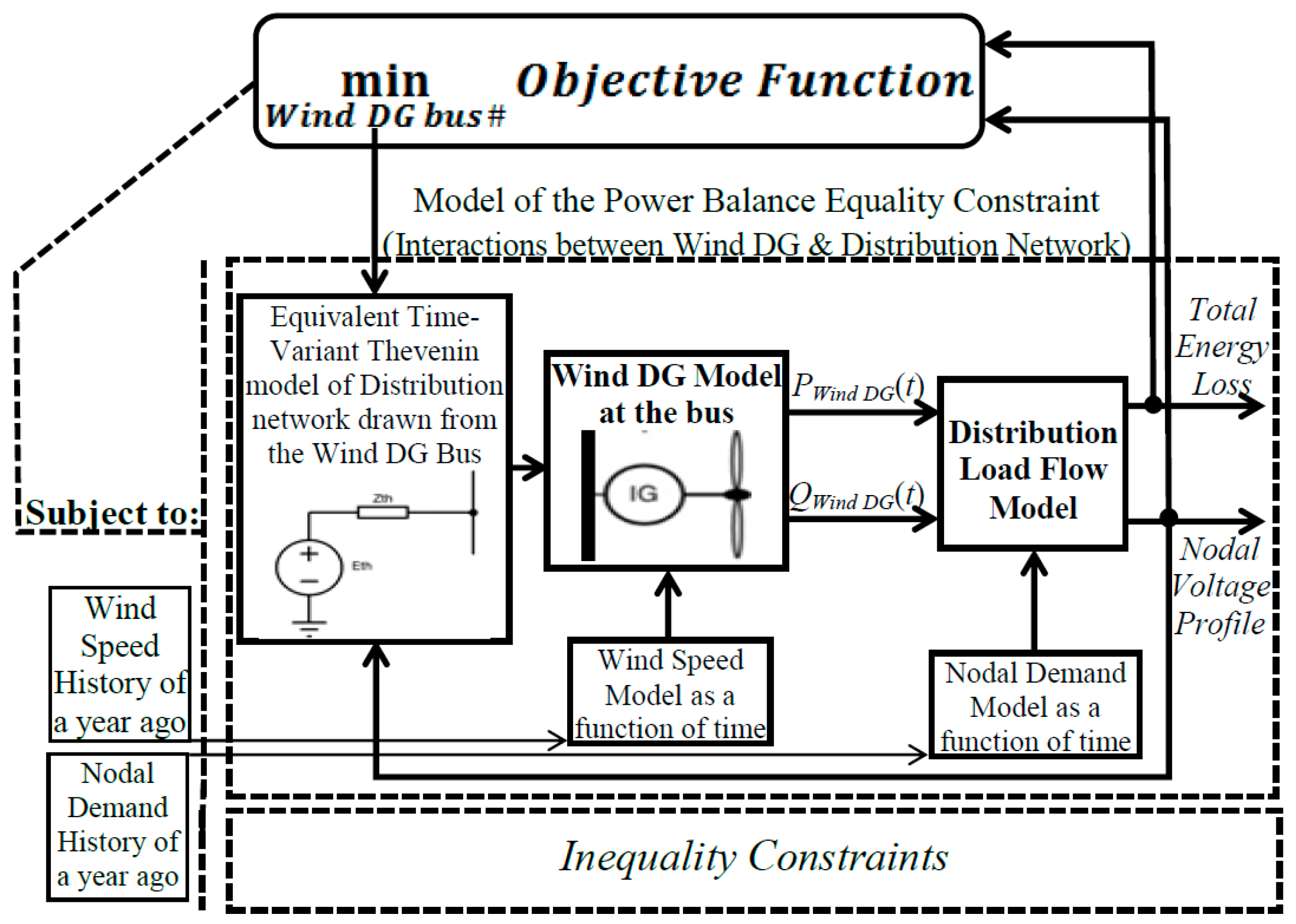
The general definition and structure of the WDG placement problem under study is illustrated in Figure 1. According to this figure, the WDG placement problem is a kind of optimization problem with some objective function and constraints. However, due to the intermittent and time-variant nature of wind speed and demand, this optimization problem cannot be directly formulated. Thus, the block diagram in Figure 1 is utilized here for the problem definition, including three principal blocks as follows:

–

The first block models the objective function.

–

The second block is treated as the main equality constraint of the optimization problem. It models the power balance constraint considering the interactions between WDG and the distribution network.

–

The third block comprises the inequality constraints of the optimization problem.

The aim of this paper is to extract the detailed models of the above three blocks, as well as to propose an efficient solution for solving the whole optimization problem. Hence, first, the detailed models of the above blocks are presented in the rest of this section.

2.1. Objective Function Model

The objective of the optimization problem is to find the optimal bus for connecting the WDG in a distribution network, to minimize the aggregate electric energy loss, as well as to achieve a smooth nodal voltage profile with less total deviation from 1 p.u during the planning period. This objective function is formulated in Equation (1), where symbols E_LossWithDG and VD_WithDG denote the aggregate electric energy loss and voltage deviation criteria in the system with the WDG, respectively. The E_LossNoDG and VD_NoDG are similar variables in the system without the WDG. V_{bus I,WithDG,t} and P_LossWithDG,t are the voltage magnitude of bus i, and the entire active power loss in the system with the WDG, and in the sampling interval t, respectively. Similarly, V_{bus i,NoDG,t} and P_LossNoDG,t represent similar variables for the case without the WDG. Finally, F is the resultant objective function. The entire voltage deviation index is defined according to Equation (2), with symbol V_{bus i,t} representing the voltage magnitude of bus i in the sampling interval t, and in either of the two cases (with or without the WDG).

$$F=\frac{E_{LossWithDG}}{E_{LossNoDG}}+\frac{V{D}_{WithDG}}{V{D}_{NoDG}}=\frac{{\displaystyle \sum _{\mathrm{All}\mathrm{times}t}{P}_{LossWithDG,t}}}{{\displaystyle \sum _{\mathrm{All}\mathrm{times}t}{P}_{LossNoDG,t}}}+\frac{{\displaystyle \sum _{\mathrm{All}\mathrm{times}t}{\displaystyle \sum _{AllBuses}\left|V_{busi,WithDG,t}-1\right|}}}{{\displaystyle \sum _{\mathrm{All}\mathrm{times}t}{\displaystyle \sum _{AllBuses}\left|V_{busi,NoDG,t}-1\right|}}}$$

(1)

$$VD={\displaystyle \sum _{\mathrm{All}\mathrm{times}t}{\displaystyle \sum _{AllBuses}\left|V_{busi,t}-1\right|}}$$

(2)

It is observable that in Equation (1) the values for the system, with the WDG, are divided by the corresponding values for the system without the WDG. The reason for this is to homogenize the two terms of the objective function so that they both have similar dimensions. Moreover, since the problem under study just considers the optimal placement of WDG (assuming a fixed power capacity for it), the investment cost of WDG is unimportant and is disregarded here.

2.2. Model of the Power Balance Constraint (Interactions between WDG and Network)

As is seen in Figure 1, the most significant block of the WDG placement problem under study, is the model of the power balance constraint, treated as the main equality constraint of the optimization problem. In this block, the time-dependent input data for the optimization problem are produced by using the models of time-variant nodal demands and wind speed. These models extract the “typical nodal demands and wind speed patterns” as some functions of time from those historical data in a way that will be described in next section. The resulted data are applied to the models of distribution load flow, and WDG is connected to the candidate bus of the distribution network. The distribution network behavior, as is seen from the WDG bus, is also modeled by using the equivalent time-variant Thevenin model at the WDG bus. This model is influenced by the time variations of the nodal voltage profile and the electrical location of the WDG bus itself. On the other hand, it provides the supply voltage for the WDG model, and thereby, the interactions of WDG and the distribution network are well-regarded. The WDG model calculates the time-variant active and reactive power injections from the WDG to the network (i.e., P_WDG(t) and Q_WDG(t) in Figure 1). These variables participate in the distribution load flow model as the kernel of the power balance constraint. By solving the distribution load flow problem, for all the sampling intervals during the planning period, the nodal voltage profiles and the values of the active power loss in each interval can be elucidated. These results not only are utilized in the objective function formulation, but also affect the equivalent time-variant Thevenin model at the WDG bus, and, consequently, the outputs of the WDG model (especially the reactive power exchange between the WDG and network). This feedback loop evidently demonstrates the high complexity of the defined power balance constraint block, as the principal equality constraint of the optimization problem under study. In other words, such an equality constraint is indeed a complicated time-variant model that necessitates using the new proposed algorithm or the solution.

2.3. Models of Time-Variant Wind Speed and Nodal Demands

Here, the time-profiles of input data (i.e., wind speed and nodal demands) are modeled regarding the fact that the WDG placement problem is indeed a type of planning problem, in which the long-term behaviors of the input data should be taken into account. In addition, time variations of such variables mostly follow approximate diurnal (24 h) patterns; of course with some random variability. This is mainly because of the sun radiation diurnal pattern influencing the time variations of the others. Additionally, wind speed also has a different typical diurnal pattern, dependent on the seasonal and geographical conditions. Nevertheless, it is impossible to consider all individual hours of a year in the simulation process, since it takes a long solution time. Here, a good alternative is to define and obtain the ‘typical’ or ‘average’ diurnal patterns for the input data and apply them to the simulation with 24 h (86,400 s) duration. Meanwhile, in order to regard the seasonal variations of the input signals, such average diurnal profiles are extracted for each month in a year, and all are then applied to the simulation, successively. Thus, the simulation is repeatedly run 12 times, each with 24 h (86,400 s) duration and its own applied 24 h input data. The average diurnal patterns are all formulated as some appropriate mathematical expressions by using the curve fitting technique, so as to simplify the simulation model and reduce its runtime, as described in the following sections.

2.4. Monthly Average Diurnal Wind Speed Patterns

According to the above considerations, each of the monthly average diurnal wind speed patterns is defined as the 24 h profile of the hourly mean values, obtained through averaging all the wind speeds of that hour across the 30 days interval of the associated month, as formulated in Equation (3). In this formula, v_m(h,d) stands for the wind speed in hour (h) of the day (d), and month (m), while ${\overline{v}}_m\left(h\right)$ represents the resulted average wind speed corresponding, to the hour (h) of the typical day in month m. Accordingly, ${\overline{v}}_{Load,1}\left(h\right)$ to ${\overline{v}}_{Load,12}\left(h\right)$ symbolize all the monthly load profiles resulted for each of the 12 months of the year.

$${\overline{v}}_m(h)=\frac{1}{30}{\displaystyle \sum _{d=1}^{30}{v}_m(h,d)},h=1,2,\dots ,24,m=1,2,\dots ,12$$

(3)

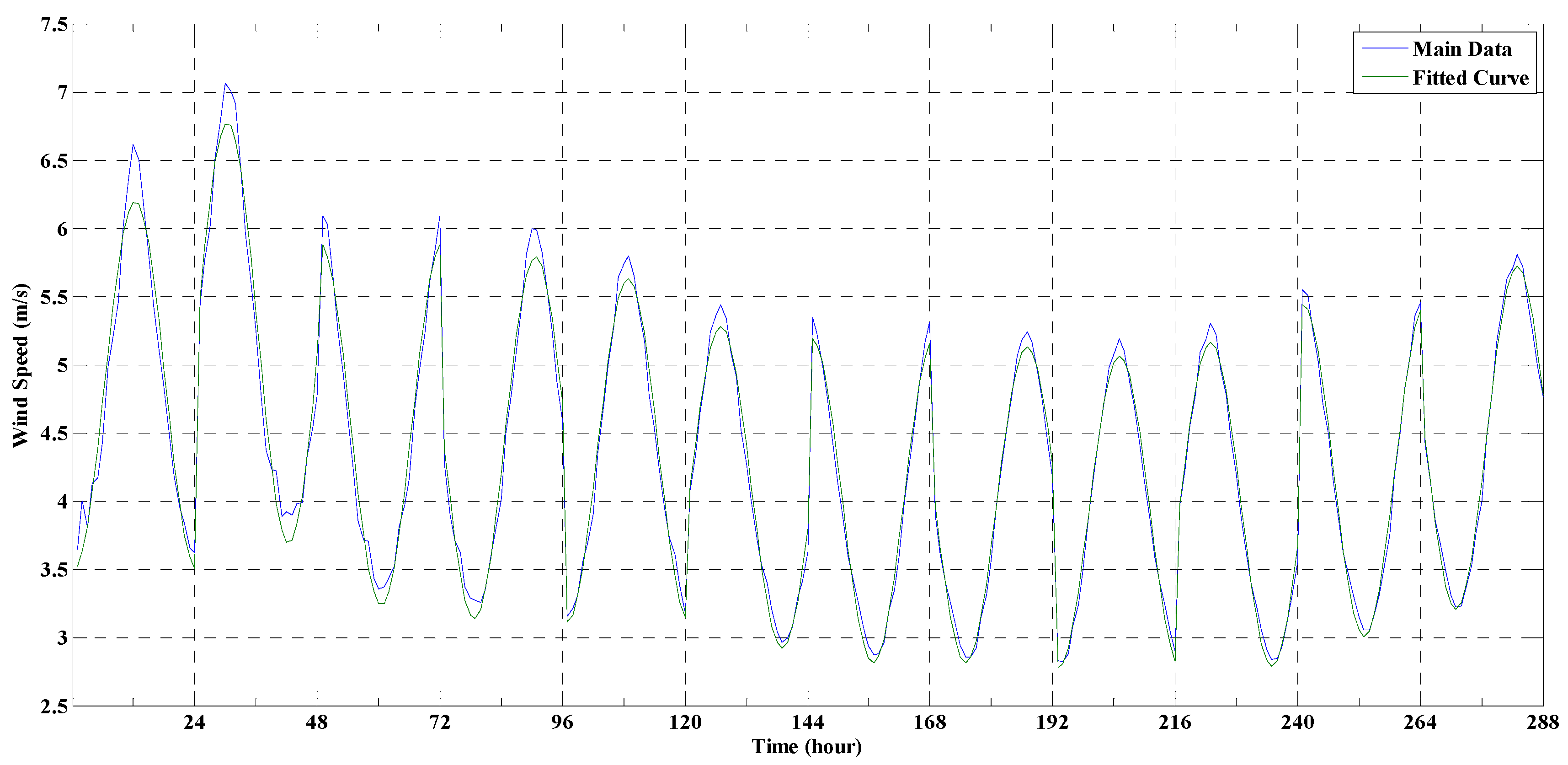
As described before, for the purpose of simplification, the monthly average diurnal wind speed patterns are approximated by some mathematical formulations using the curve fitting technique. According to the inherent nature of wind speed profiles, the monthly average diurnal wind speed patterns typically have just one peak, and therefore, they can be best approximated via using a single biased sinusoidal function, as formulated in Equation (4) [22].

$${\overline{v}}_m(h)={\overline{V}}_m\left\{1+\delta \cos \left[\left(\frac{2\pi }{24}\right)\left(h-\phi \right)\right]\right\}h=1,2,\dots ,24$$

(4)

where, ${\overline{v}}_m$, δ, and ϕ denote the overall average wind speed in month m, the magnitude of sinusoidal function (called ‘diurnal pattern strength’), and its phase shift hour (called ‘mean hour of peak wind speed’), respectively, and ${\overline{v}}_m\left(h\right)$ yields the mean wind speed in hour h of the typical day in month m as a sinusoidal function of hour (h). The resulted monthly wind speed profiles exploited in this paper are all depicted in Figure 2 beside their associated fitted curves.

The monthly sinusoidal functions fitted to the monthly average diurnal wind speed patterns are all utilized consecutively in the simulation process to form the wind speed input signal of the wind turbine. Thus, not only are both the average diurnal and seasonal behaviors of wind speed perfectly modeled without a long solution time, but also, the sudden and sharp variations of wind speed are not modeled. Thereby, the output power of the WDG is obtained according to the average long-term behavior of wind speed. This is in agreement with the inherent definition of the DG placement process, having a planning and long-term nature, as explained earlier.

2.5. Monthly Average Diurnal Demand Patterns

Similar to the previously defined wind speed patterns, each of the monthly average diurnal demand patterns is defined as the 24 h profile of the hourly mean values. Each value is obtained by averaging all the demand values of that hour across the 30-day interval of the associated month. This definition is formulated in Equation (5), where P_Load,m(h,d) denotes the power demand in hour h of day d and month m, and ${\overline{P}}_{Load,m}\left(h\right)$ represents the resulted average power demand corresponding to hour h of a typical day in month m. Thus, ${\overline{P}}_{Load,1}\left(h\right)$ to ${\overline{P}}_{Load,12}\left(h\right)$ encompass all of the monthly profiles resulting from each of the 12 months in a year.

$${\overline{P}}_{Load,m}(h)=\frac{1}{30}{\displaystyle \sum _{d=1}^{30}{P}_{Load,m}(h,d)},h=1,2,\dots ,24,m=1,2,\dots ,12$$

(5)

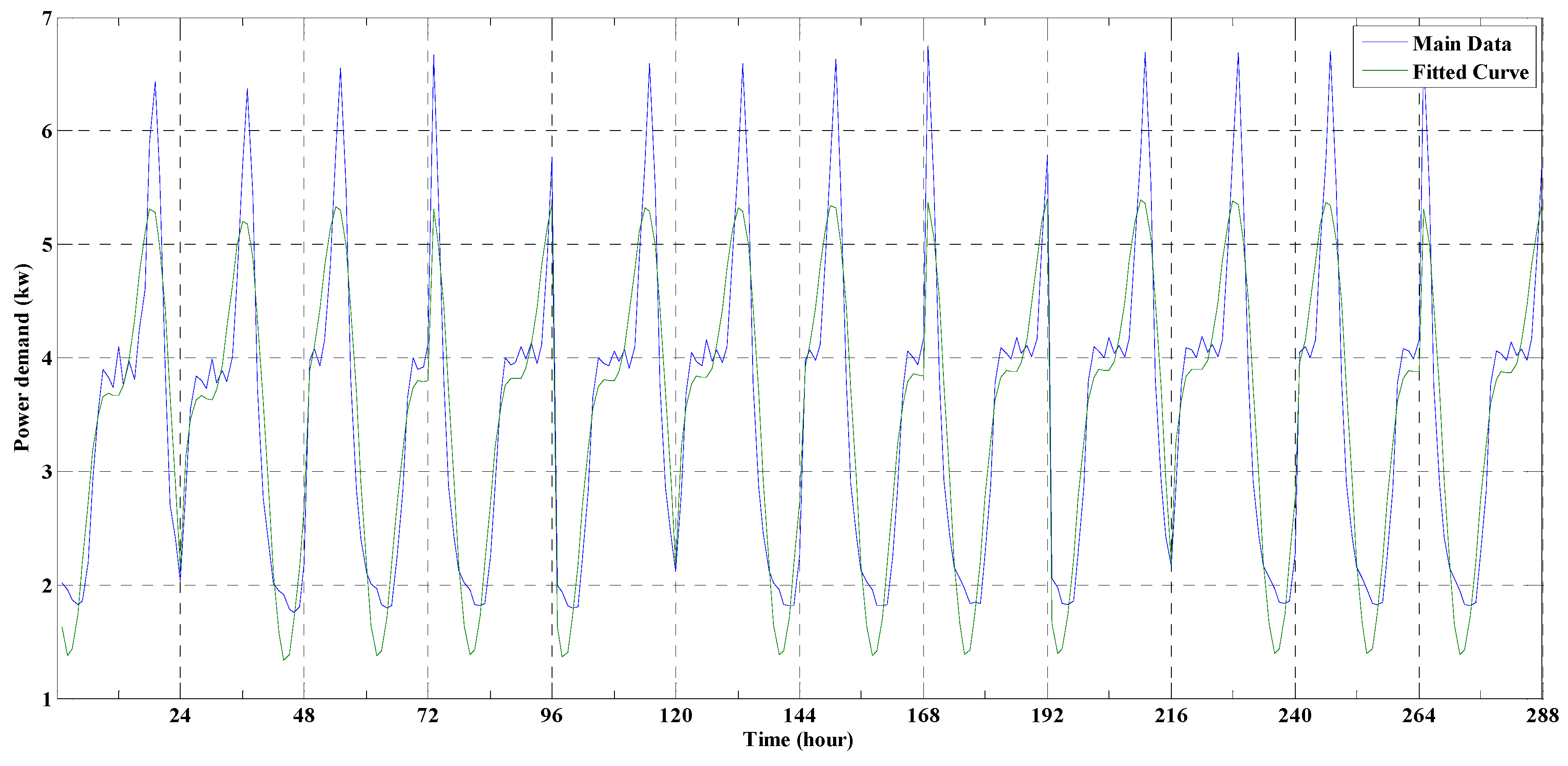
Like the diurnal wind speed patterns, for sake of simplification, the average diurnal demand patterns should be approximated by some mathematical formulations via using the curve fitting technique. Due to the inherent nature of non-industrial demands, such profiles mostly have two (minor and major) peaks. On the other hand, such profiles all have daily periodic natures, i.e., the power demand at the beginning of the day habitually equals t at the end of day (${\overline{P}}_{Load,m}\left(0\right)={\overline{P}}_{Load,m}\left(24\right)$). Therefore, such profiles can be best approximated using a two-term Fourier series, as formulated in Equation (6), in which symbols t and ${\overline{P}}_{Load,m}\left(t\right)$ denote the time (in hours or any other appropriate units), and the average demand (in kW) belonging to time t and month m, respectively. Additionally, parameters a₀ to a₂ and b₁ to b₂ are the Fourier coefficients, and ω is the fundamental angular frequency of the signal that is determined according to the signal period (i.e., one day or 24 hours), as seen in Equation (6). The resulted monthly demand profiles that are utilized in this paper are all depicted in Figure 3 beside their associated fitted curves.

$$\begin{array}{l}{\overline{P}}_{Load,m}(t)=a_0+a_1\cos (\omega t)+b_1\sin (\omega t)+a_2\cos (\omega t)+b_2\sin (\omega t)\\ \omega =\frac{2\pi }{24}\left(\raisebox{1ex}{$rad$}\!\left/ \!\raisebox{-1ex}{$hours$}\right.\right)\end{array}$$

(6)

As this paper considers a distribution network for the WDG placement analysis, it is necessary to provide some nodal load profiles; each having some similar forms to those illustrated in Figure 3. Then, in the numerical analysis section, the default nodal loads are all modified according to Equation (7), where ${\overline{P}}_{Load i, m}\left(t\right)$ and $P_{Load i, defult}$ represent the average diurnal load profile applied to bus (i) in month m, and the previous default load at bus (i), respectively. This equation can be used for both active and reactive nodal loads.

$${\overline{P}}_{Loadi,m}(t)=\frac{a_0+a_1\cos (\omega t)+b_1\sin (\omega t)+a_2\cos (\omega t)+b_2\sin (\omega t)}{a_0}{P}_{Loadi,default}$$

(7)

As is illustrated in Figure 1, the above nodal loads are not directly modeled in the simulation of the grid-connected WDG, but instead, they are regarded in the distribution load flow calculation according to the way described in Section 3. The distribution load flow subsequently yields some, monthly average diurnal nodal voltage patterns, corresponding to each of the monthly average diurnal demand patterns, and such resulted voltage patterns for the candidate bus of WDG are modeled in the simulation of the grid-connected WDG, as described in the section below.

2.6. Equivalent Time-Variant Thevenin Model of Distribution Network Drawn from the WDG Bus (Monthly Average Diurnal Grid Voltage Patterns)

The power grid is modeled here, as a time-variant equivalent Thevenin circuit for the base power system (without DG), drawn from the bus at which the WDG is going to be connected. As illustrated in Figure 1, it is composed of a time-variant Thevenin voltage source together with fixed Thevenin impedance, respectively derived from the calculations of distribution load flow and the impedance matrix in the base power system, without WDG. The time-variant Thevenin voltage source models the time variations of the candidate bus voltage, before connecting to the WDG. Thus, by applying the monthly average diurnal demand profiles, the nodal voltage profiles (resulted from distribution load flow calculations) also follow from some similar monthly average diurnal patterns. Hence, the time-variant voltage profile resulted for the candidate bus per hour of the typical day is applied to the Thevenin voltage source in the simulation process (Figure 1).

2.7. Grid-Connected WDG Model

The grid-connected WDG system is simulated here via a simulation scheme including a simple Squirrel-cage Induction Generator driven by a wind turbine [23] and directly connected to the candidate bus of the distribution network (with the equivalent time-variant Thevenin model). The wind turbine can be considered either with the pitch angle controlling system or without it. The wind turbine-induction generator (WT-IG) model can completely be extracted from [24].

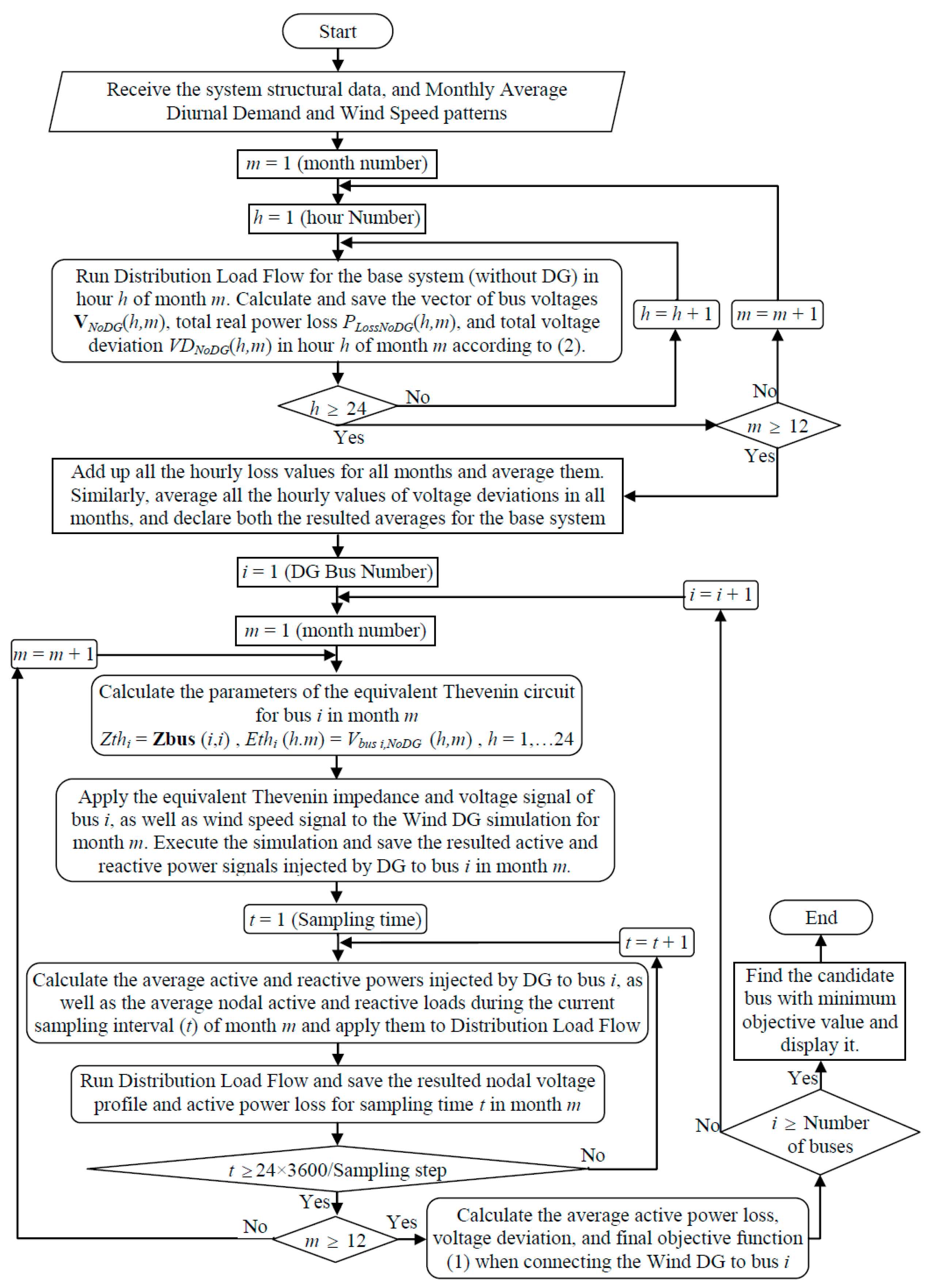
3. Distribution Load Flow Model and Solution Algorithm

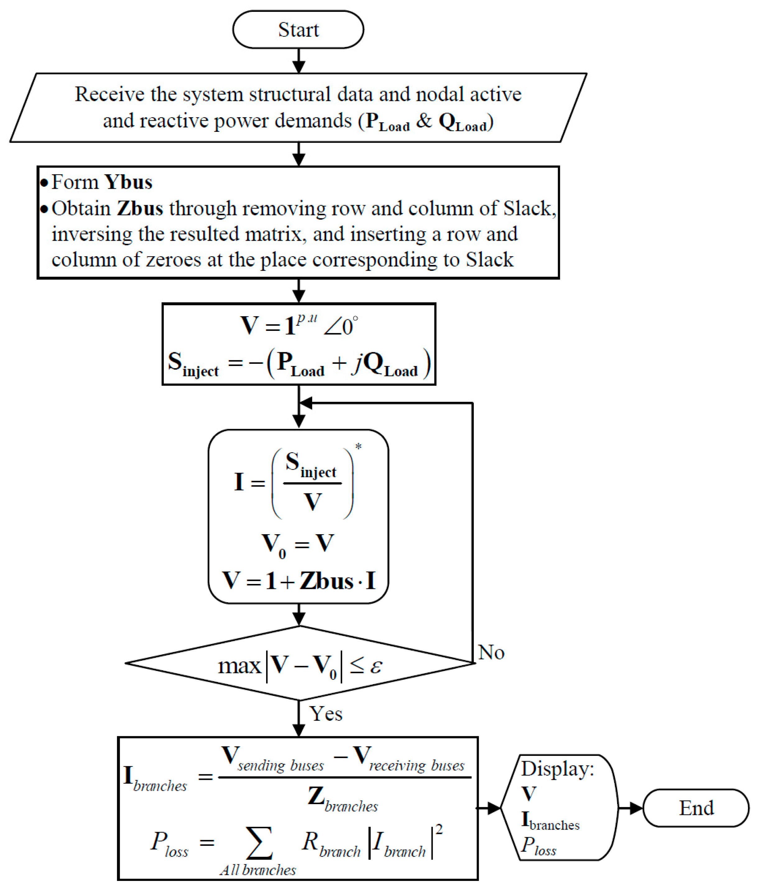
In the proposed WDG placement algorithm, the static operation state of the distribution network is modeled by a load flow problem, which is solved using a distribution load flow algorithm, as depicted in the flowchart of Figure 4. This algorithm is extracted from a past paper [14] and is utilized here by applying some extra simplifications, to reduce its solution time without impairing its accuracy. According to the flowchart of Figure 4, the utilized procedure initially forms the admittance matrix (Ybus) from the network structural data and extracts the impedance matrix (Zbus) from Ybus. This is done by removing the row and column corresponding to the slack bus in Ybus, inverting the remainder matrix, and inserting a row and column of all zeroes into the resultant inversed matrix at the place of slack. Then, at the beginning of the iterative procedure, constant nodal voltages (V), all equal to $1^{p.u}\angle 0^{\circ }$ are assumed, and the nodal injective apparent powers are calculated. In each step, the solution procedure repeatedly computes the nodal injective currents (I) from the nodal injective apparent powers and the resulting nodal voltages, and updates the nodal voltages by multiplying by Zbus. This iterative process is continued until the maximum change in nodal voltages between two successive steps reaches under a predetermined tolerance (ε). Finally, the branch currents and the total active power loss in the entire distribution network are obtained using Equations (8) and (9), respectively. Where, I_branches and Z_branches denote the vectors of branch currents and impedances, respectively and V_{sending buses} and V_{receiving buses} are the voltage vectors of sending and receiving nodes corresponding to each branch, respectively. Additionally, I_branch and R_branch are the current and resistance of each branch in the above vectors, while P_loss denotes the resulted active power loss.

$$I_{branches}=\frac{V_{sendingbuses}-V_{receivingbuses}}{Z_{branches}}$$

(8)

$$P_{loss}={\displaystyle \sum _{Allbranches}{R}_{branch}{\left|I_{branch}\right|}^2}$$

(9)

Model of the Inequality Constraints

As described before, the WDG placement problem under study is an optimization problem with just one decision variable: the WDG bus number. On the other hand, the proposed objective function perfectly regards the time-variant nodal voltage profiles and tries to smooth them with as few deviations from 1 p.u as possible. The inequality constraints associated with the allowable ranges of the active and reactive power exchanges between the WDG and distribution network are completely considered in the simulation process of the grid-connected WDG. Therefore, there is no need to regard the nodal voltage profiles and the active and reactive power exchanges of the WDG separately in the inequality constraints block. Hence, the only significant inequality constraint that remained is related to the allowable range of the WDG bus number, that is, between one, and the number of buses in the whole distribution network.

4. Proposed Solution Algorithm for the WDG Placement Problem under Study

In this section, the proposed solution algorithm for the intended WDG placement problem is presented. The fundamental concept of this algorithm is based on the superposition theorem. According to this theorem, the effects of both the time-varying power demands and wind speed can be handled in this way: At first with the base distribution network with time-varying loads, but without WDG, with the distribution load flow calculation and the nodal voltages result. From the viewpoint of the candidate bus for the WDG placement, the voltage obtained above is treated as the open-circuit, or no-load voltage, which makes the Thevenin source voltage profile. Then, by connecting the WDG to the candidate bus, the distribution network is abandoned, and its behavior is completely modeled by the Thevenin voltage source. Therefore, the actual voltage variations of the WDG bus during its operation is calculated in the simulation process, and the time-varying profiles of the active and reactive powers, injected by the WDG to the distribution network, are obtained as well. The proposed solution procedure is graphically scheduled in the flowchart of Figure 5. Accordingly, the optimization problem was solved by using the direct search method. Consequently, all the system buses are tried consecutively for DG placement; no stochastic search methods were used. In this way, the inequality constraint of the allowable range of the WDG bus number is automatically satisfied too.

5. Numerical Analysis

The proposed WDG placement algorithm is applied to the radial 33-bus distribution test network, presented previously [14,21], via programming in MATLAB. On the other hand, the WDG under study is of 1.5 MW capacity with base wind speed equal to 6 m/s. It was modeled using Simulink and is then linked to the main written program. Thus, the simulation was run via calling during the main program procedure, wherever needed, as described in Section 3. The performance of the proposed algorithm is verified here by comparing the results with the conventional DG placement algorithm. The DGs with renewable energy resources were simply modeled as fixed active and reactive generation sources (or fixed negative active and reactive demands). In this way, the mentioned 33-bus distribution test system is considered, with near-actual demand and wind speed data, adopted from two template files of HOMER software.

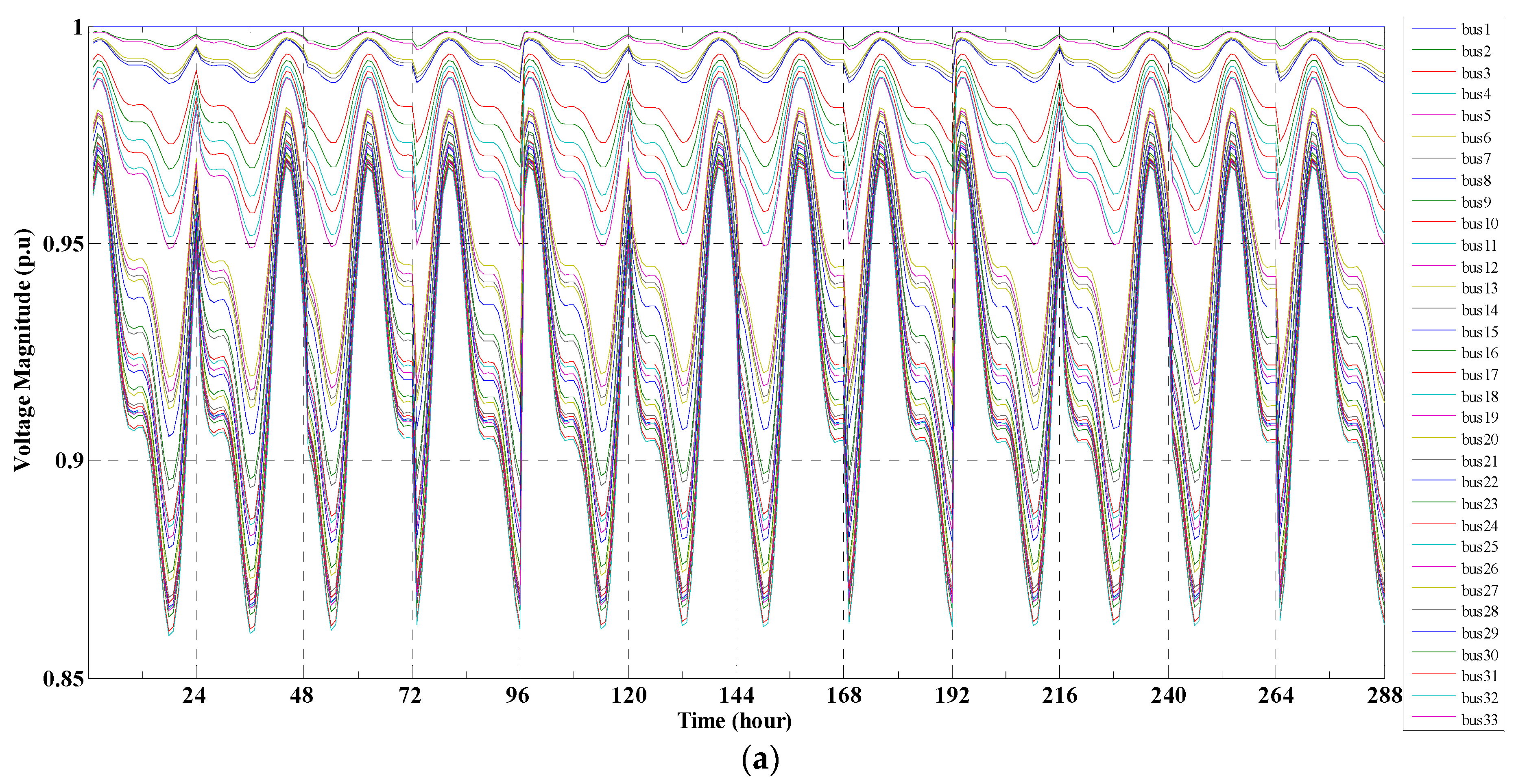
They contain 8760 sample data per hour of a year, respectively, corresponding to power demand and wind speed values during a year. By using these data, the monthly average diurnal demand, and wind speed patterns are calculated according to the methods described in Section 2, as illustrated in the graphs of Figure 2 and Figure 3, respectively. The nodal active and reactive demands for all the 33 buses in the 33-bus distribution network were extracted from the above-mentioned sample demand data according to Equation (8). The resulted monthly average diurnal patterns for all the nodal active and reactive demands are given to the proposed algorithm. 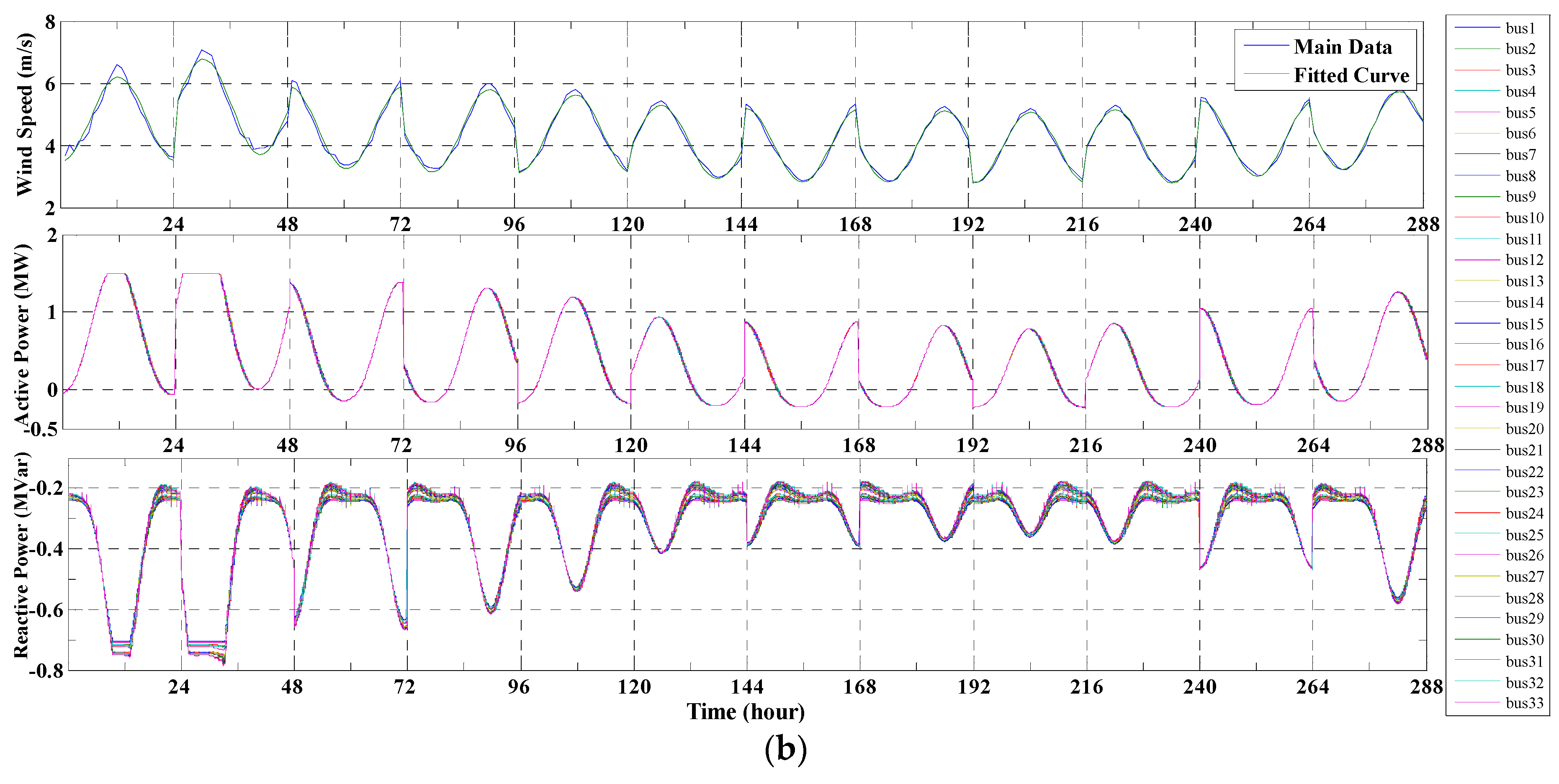Accordingly, by performing the successive power flow analyses in the base distribution system without WDG, all the monthly average diurnal Thevenin source voltage profiles, for all the 33 buses, were obtained and simultaneously plotted in the graphs of Figure 6a. After running the proposed placement algorithm, all the monthly average diurnal patterns of the active and reactive powers injected by the WDG, when connecting to each of the 33 buses in the distribution network, are available as plotted in Figure 6b (beside the graphs of the monthly average diurnal wind speed patterns, in order to achieve more clearness). With the attention to these three plots, it is observable that the variations of the active power injected by the WDG are mostly in direct proportion to the wind speed variations. Although the active power injection of WDG mostly has positive values, it may display negative values (i.e., a motor operation) when the wind speed faces significant drops. On the contrary, the active power injection of the WDG, approximately, has similar behaviors when the WDG is connected to each of the different buses in the system. This implies that the variations of the WDG active power injection are not greatly affected by the different voltage magnitudes in the different buses. On the other hand, the reactive power injection has a different behavior. According to Figure 6b, it is obvious that the reactive power injection always has negative values (because of the inherent characteristic of induction generator). In other words, the Induction machine-WDG always consumes some reactive power. The reactive power consumption level is in direct proportion to the wind speed, and reverse proportion to the bus voltage magnitude, as seen in Figure 6b. It increases wherever the wind speed increases and has lower values for the nodes with higher voltage magnitudes (e.g., the first nodes near to the Slack bus).

The main outcome, of any DG placement procedure, is to find the best bus to which the DG should be connected. After running the proposed WDG placement algorithm, bus 12 was obtained as the best candidate bus, while using the conventional algorithm [14] (in which the WDG is treated as a fixed load demand), bus 18 was determined to be the best. As presented in a previous paper [14], the modeling of WDG is based on the time-varying DG source and it is simulated based on statistical wind data. Therefore, the effect of the dynamic model has not been considered in the placement process. Moreover, in this paper, only the annual daily average output power profile of WDG with the daily average demand of a typical house has been regarded.

The main outcomes of the two approaches, as well as those of the base system without WDG, are illustrated in

Table 1. Comparison of the main outcomes of the conventional [14] and proposed WDG placement algorithms, along with the corresponding results of the base system without WDG.

Case of Analysis Resulted Variable	Base System without WDG	New Algorithm	Conventional Algorithm [14]
Optimal Bus for Connecting the WDG	-	12	18
Overall Average Active Power Loss in kW	235.5	223.0	238.5
Overall Average Voltage Deviation Index in p.u	0.0521	0.0485	0.0485
Resulted Global Objective Value	2	1.8778	1.9419

. It clearly demonstrates the effectiveness of the proposed WDG placement mechanism, as it yields lower values for the global objective function in Equation (1) and the average active power loss. However, a comparison of the resulted voltage profile and active power loss between the two cases of using either of the two algorithms can further prove the merit of the newly proposed algorithm.

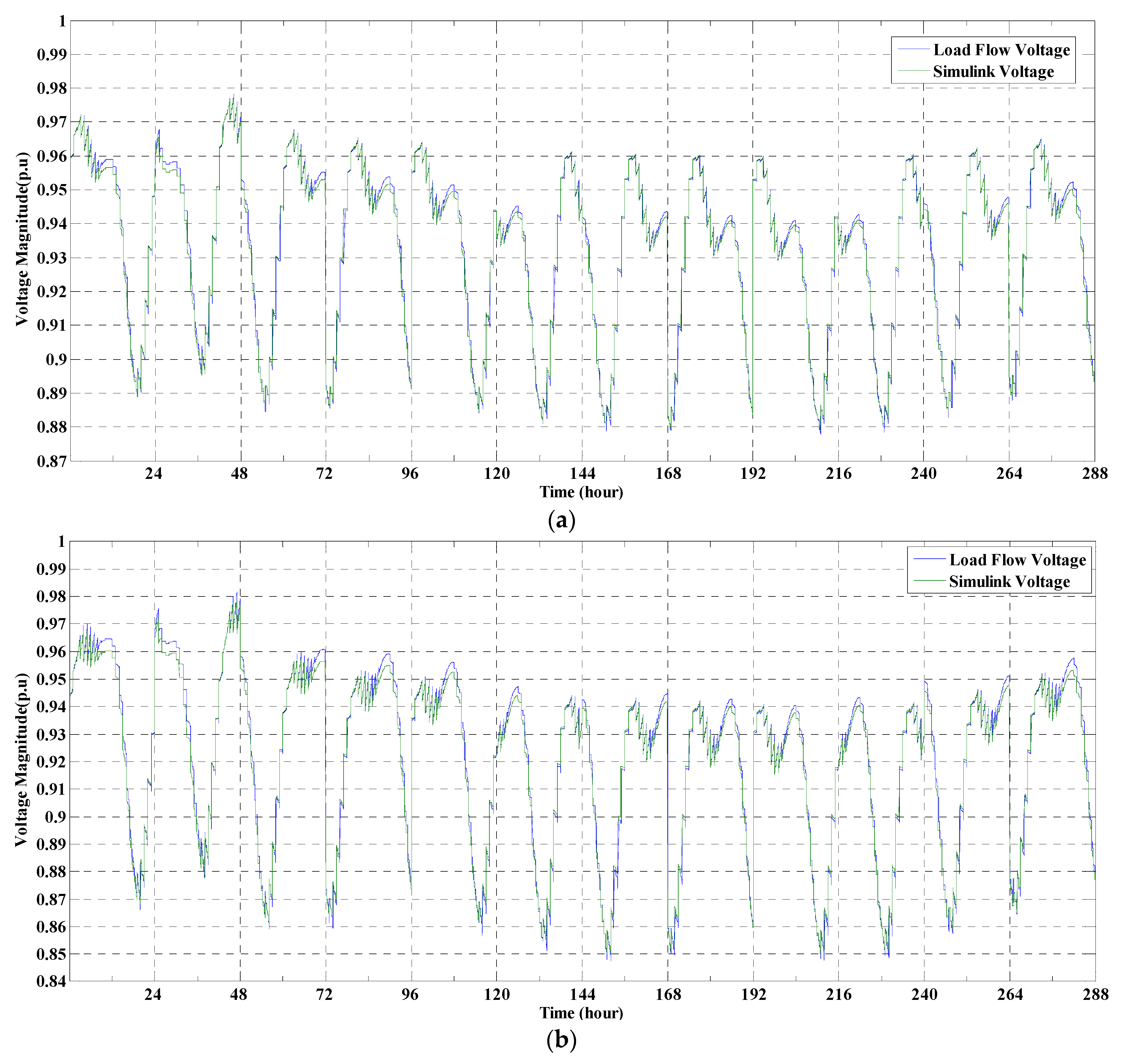
Accordingly, Figure 7a displays the resultant monthly average diurnal voltage profiles of bus 12 when connected to the WDG. In contrast, Figure 7b illustrates a similar profile for bus 18 when the bus is instead connected to the WDG. Figure 7c illustrates the monthly average diurnal active power loss patterns resulted from each of the three cases: the base distribution system without WDG, the system with the WDG connected to bus 12, and the system with the WDG connected to bus 18. According to Figure 7, WDG placement based on the new algorithm proposed in this paper yields better results, from the viewpoints of voltage profile smoothness and of active power loss reduction. Moreover, in Figure 7a,b the voltage profiles resulted from the simulation models are plotted together with those obtained from the load flow calculations, separately for the cases of connecting the WDG to buses 12 and 18, respectively. For more clarity, the graphs of bus 18 are replotted in Figure 7d beside the Thevenin source voltage profile at bus 18 (i.e., the voltage profile of bus 18 when not connected to the WDG). According to these figures, the voltage profile of the WDG bus resulted from the simulation model exactly coincides with that resulted from the distribution load flow calculation, while the bus voltage profile in the case of not connecting to the WDG is obviously different. This strongly validates the concept of the proposed WDG placement mechanism, described in Section 3. Furthermore, in Figure 7c, it is observable that the active power loss profile corresponding to the case of connecting the WDG to bus 12 (the result of the new proposed method) includes lower values than the other two profiles. Therefore, not only is the proposed WDG placement algorithm completely valid, but it also has good performance and effectiveness, as it regards all the effects of power demands as well as wind speed variations in the WDG placement algorithm.

6. Conclusions

In this paper, a new algorithm for the optimal placement of one WDG (base on induction generator) in the distribution networks has been presented to minimize the aggregate energy loss as well as the nodal voltage deviations (from 1 p.u). The proposed scheme considers the time variations of dynamic nodal demands, nodal voltage magnitudes, and wind speed in the WDG placement process altogether. By this means, an accurate dynamic model of the active and reactive powers injected by WDG to the system is employed in which the interactions between the WDG and the distribution network are well-viewed.

Accordingly, the simulation is executed for 12 typical (24 h) days, each representing a different month of the year. Thereby, the accurate time-varying model of the active and reactive powers injected by WDG to the distribution network is considered in the solution process of the placement problem. The results obtained from the numerical analysis confirm the validity, accuracy, and effectiveness of the proposed WDG placement algorithm. According to these results, unlike the conventional placement algorithms for DGs with intermittent energy resources, the new algorithm of this paper further regards the actual situations of both the distribution network and the DG system, and consequently yields much more accurate results.