Assessment and Performance Evaluation of a Wind Turbine Power Output


Abstract
1. Introduction
2. Data and Methodology
- Scenario A–u > 3.0 from t1–t60:Wind speed range above cut-in speed for the 60 time steps
- Scenario B–u < 3.0 at t1:Wind speed startup lower than cut-in speed
- Scenario C–u > 3.0 between t1–tn, u < 3.0 at tn+1:A range of lower wind speed between higher values
3. Results and Discussion
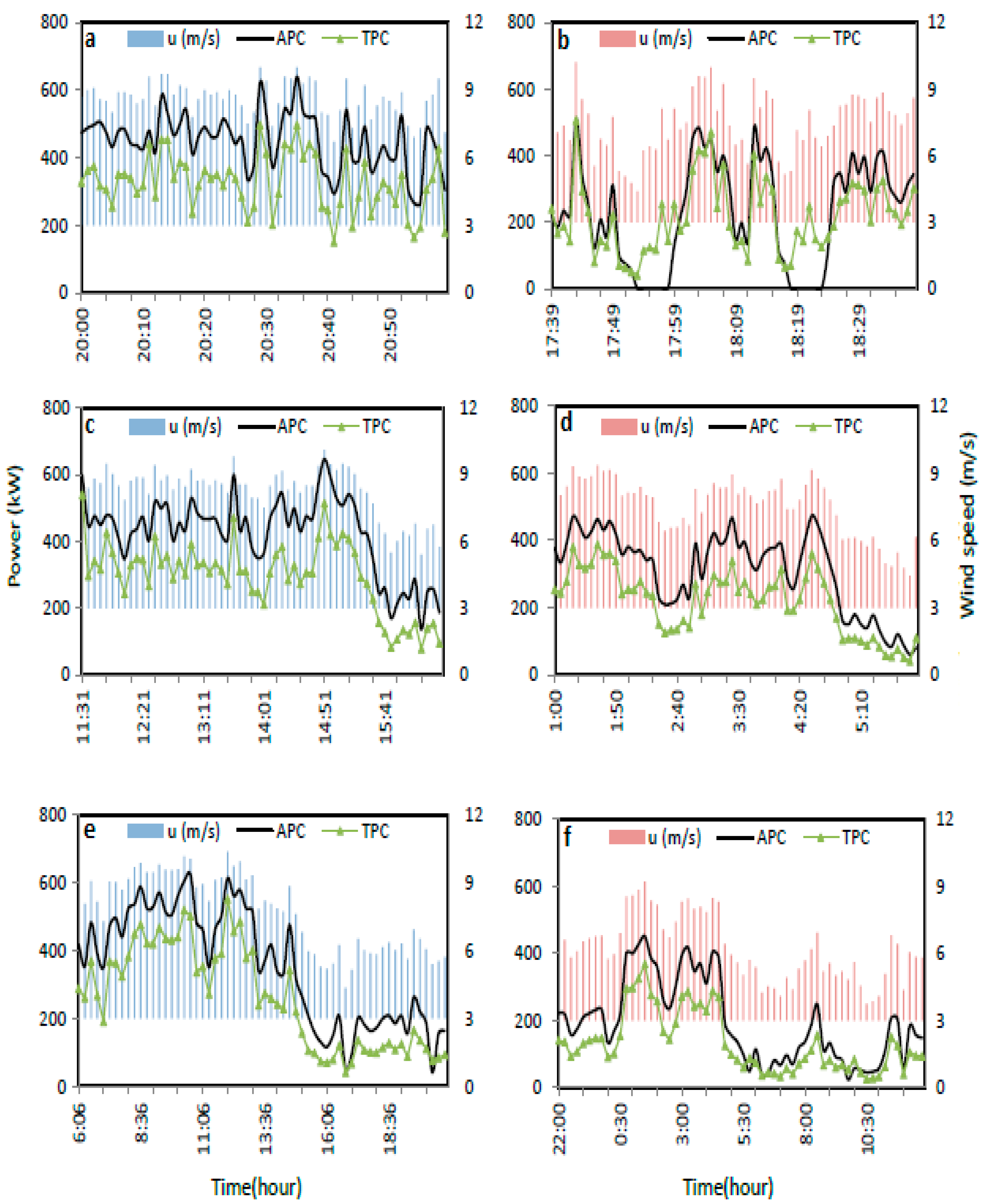
3.1. Scenario A
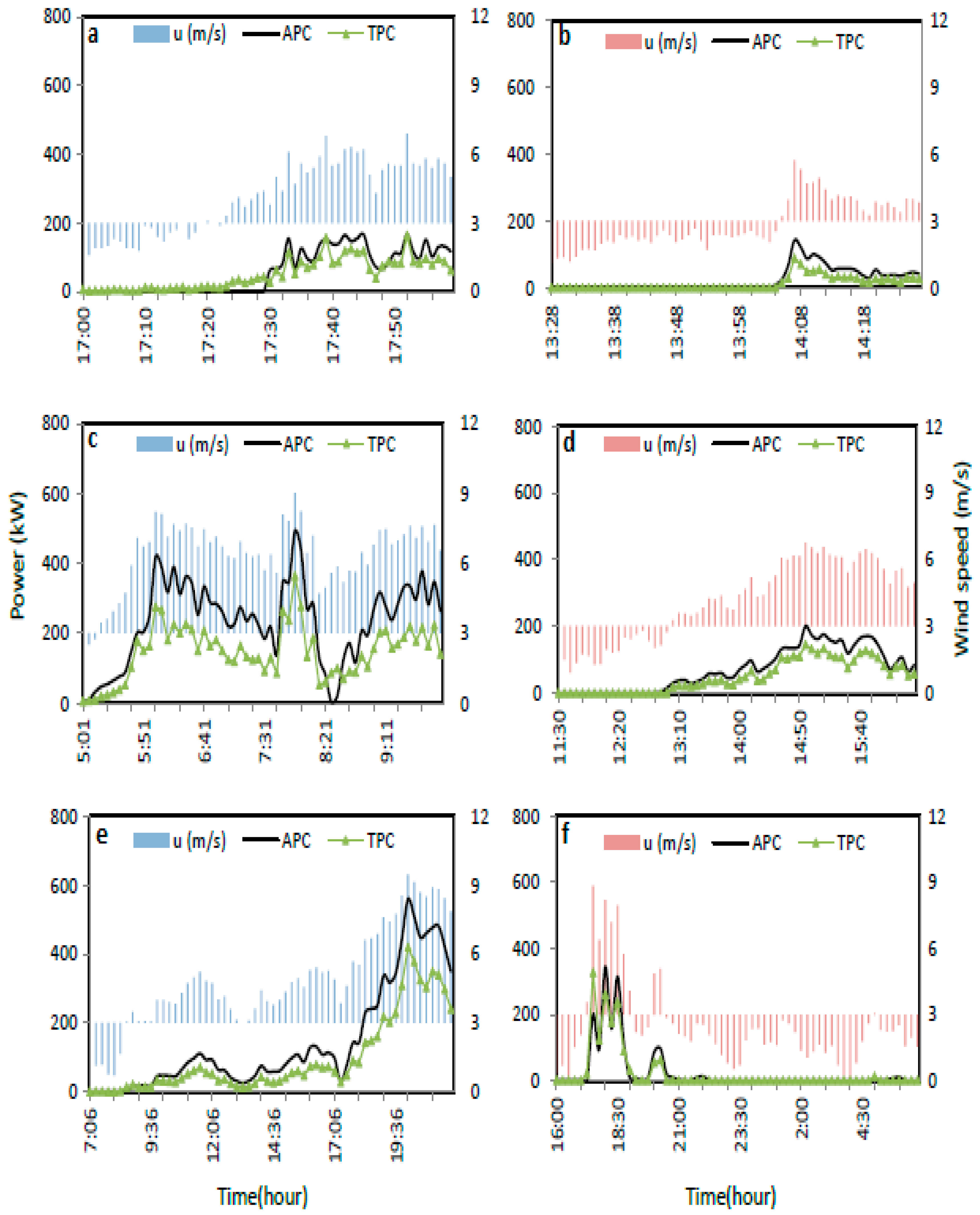
3.2. Scenario B
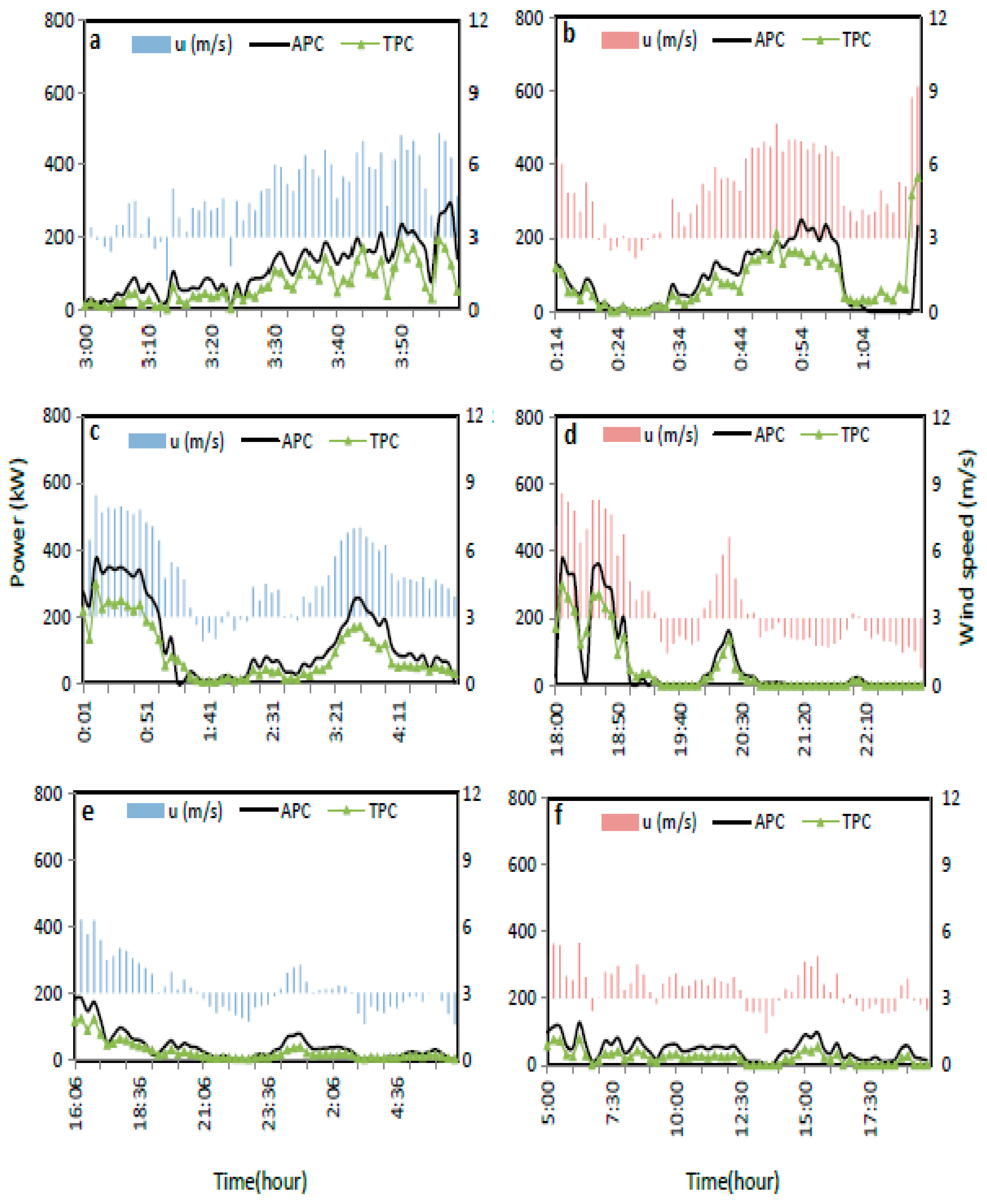
3.3. Scenario C
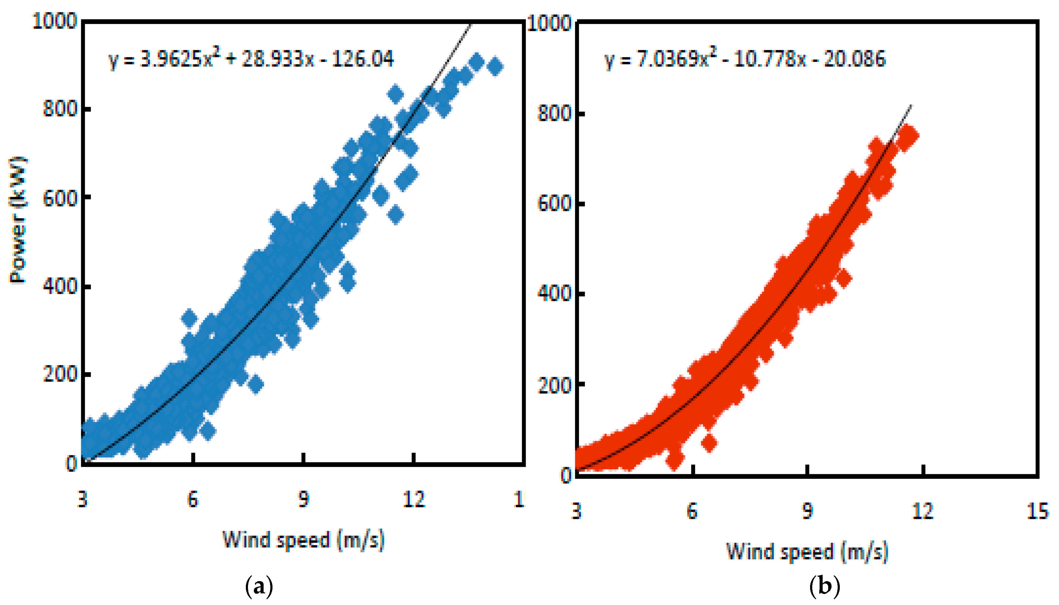
3.4. Estimations Using the Effective Power Curve
4. Conclusions
Supplementary Materials
Author Contributions
Funding
Acknowledgments
Conflicts of Interest
References
- Negnevitsky, M.; Potter, C.W. Innovative short-term wind generation prediction techniques. In Proceedings of the Power Systems Conference and Exposition, Atlanta, GA, USA, 29 October–1 November 2006; pp. 60–65. [Google Scholar]
- Valentine, S.V. A STEP toward understanding wind power development policy barriers in advanced economies. Renew. Sustain. Energy Rev. 2010, 14, 2796–2807. [Google Scholar] [CrossRef]
- Renani, E.T.; Elias, M.F.M.; Rahim, N.A. Using data-driven approach for wind power prediction: A comparative study. Energy Convers. Manag. 2016, 118, 193–203. [Google Scholar] [CrossRef]
- Bludszuweit, H.; Domínguez-Navarro, J.A.; Llombart, A. Statistical analysis of wind power forecast error. IEEE Trans. Power Syst. 2008, 23, 983–991. [Google Scholar] [CrossRef]
- García-Bustamante, E.; González-Rouco, J.F.; Jiménez, P.A.; Navarro, J.; Montávez, J.P. A comparison of methodologies for monthly wind energy estimation. Wind Energy 2009, 12, 640–659. [Google Scholar] [CrossRef]
- García-Bustamante, E.; González-Rouco, J.F.; Jiménez, P.A.; Navarro, J.; Montávez, J.P. The influence of the Weibull assumption in monthly wind energy estimation. Wind Energy 2008, 11, 483–502. [Google Scholar] [CrossRef]
- Akinsanola, A.A.; Ogunjobi, K.O.; Abolude, A.T.; Sarris, S.C.; Ladipo, K.O. Assessment of wind energy potential for small communities in south-south Nigeria: Case study of Koluama, Bayelsa State. J. Fundam. Renew. Energy Appl. 2017, 7, 1–6. [Google Scholar] [CrossRef]
- Abolude, A.; Zhou, W. A preliminary analysis of wind turbine energy yield. Energy Procedia 2017, 138, 423–428. [Google Scholar] [CrossRef]
- Villanueva, D.; Feijóo, A. Normal-based model for true power curves of wind turbines. IEEE Trans. Sustain. Energy 2016, 7, 1005–1011. [Google Scholar] [CrossRef]
- Kusiak, A. Share data on wind energy. Nature 2016, 529, 19–21. [Google Scholar] [CrossRef] [PubMed]
- Staffell, I.; Green, R. How does wind farm performance decline with age? Renew. Energy 2014, 66, 775–786. [Google Scholar] [CrossRef]
- Li, S.; Wunsch, D.C.; O’Hair, E.A.; Giesselmann, M.G. Using neural networks to estimate wind turbine power generation. IEEE Trans. Energy Convers. 2001, 16, 276–282. [Google Scholar]
- Schlechtingen, M.; Santos, I.F.; Achiche, S. Using data-mining approaches for wind turbine power curve monitoring: A comparative study. IEEE Trans. Sustain. Energy 2013, 4, 671–679. [Google Scholar] [CrossRef]
- Shokrzadeh, S.; Jozani, M.J.; Bibeau, E. Wind turbine power curve modeling using advanced parametric and nonparametric methods. IEEE Trans. Sustain. Energy 2014, 5, 1262–1269. [Google Scholar] [CrossRef]
- Long, H.; Wang, L.; Zhang, Z.; Song, Z.; Xu, J. Data-driven wind turbine power generation performance monitoring. IEEE Trans. Ind. Electron. 2015, 62, 6627–6635. [Google Scholar] [CrossRef]
- Cooney, C.; Byrne, R.; Lyons, W.; O’Rourke, F. Performance characterisation of a commercial-scale wind turbine operating in an urban environment, using real data. Energy Sustain. Dev. 2017, 36, 44–54. [Google Scholar] [CrossRef]
- Lei, M.; Shiyan, L.; Chuanwen, J.; Hongling, L.; Yan, Z. A review on the forecasting of wind speed and generated power. Renew. Sustain. Energy Rev. 2009, 13, 915–920. [Google Scholar] [CrossRef]
- Foley, A.M.; Leahy, P.G.; Marvuglia, A.; McKeogh, E.J. Current methods and advances in forecasting of wind power generation. Renew. Energy 2012, 37, 1–8. [Google Scholar] [CrossRef]
- Riahy, G.H.; Abedi, M. Short term wind speed forecasting for wind turbine applications using linear prediction method. Renew. Energy 2008, 33, 35–41. [Google Scholar] [CrossRef]
- Kavasseri, R.G.; Seetharaman, K. Day-ahead wind speed forecasting using f-ARIMA models. Renew. Energy 2009, 34, 1388–1393. [Google Scholar] [CrossRef]
- Erdem, E.; Shi, J. ARMA based approaches for forecasting the tuple of wind speed and direction. Appl. Energy 2011, 88, 1405–1414. [Google Scholar] [CrossRef]
- Chen, P.; Pedersen, T.; Bak-Jensen, B.; Chen, Z. ARIMA-based time series model of stochastic wind power generation. IEEE Trans. Power Syst. 2010, 25, 667–676. [Google Scholar] [CrossRef]
- Lind, P.G.; Herráez, I.; Wächter, M.; Peinke, J. Fatigue load estimation through a simple stochastic model. Energies 2014, 7, 8279–8293. [Google Scholar] [CrossRef]
- Lind, P.G.; Vera-Tudela, L.; Wächter, M.; Kühn, M.; Peinke, J. Normal Behaviour Models for Wind Turbine Vibrations: Comparison of Neural Networks and a Stochastic Approach. Energies 2017, 10, 1944. [Google Scholar] [CrossRef]
- Simani, S.; Farsoni, S. Fault Diagnosis and Sustainable Control of Wind Turbines: Robust Data-Driven and Model-Based Strategies; Butterworth-Heinemann: Oxford, UK, 2018. [Google Scholar]
- Milan, P.; Wächter, M.; Peinke, J. Stochastic modeling and performance monitoring of wind farm power production. J. Renew. Sustain. Energy 2014, 6, 033119. [Google Scholar] [CrossRef]
- Zanon, A.; De Gennaro, M.; Kühnelt, H. Wind energy harnessing of the NREL 5 MW reference wind turbine in icing conditions under different operational strategies. Renew. Energy 2018, 115, 760–772. [Google Scholar] [CrossRef]
- Doherty, R.; O’Malley, M. A new approach to quantify reserve demand in systems with significant installed wind capacity. IEEE Trans. Power Syst. 2005, 20, 587–595. [Google Scholar] [CrossRef]
- Kaldellis, J.K.; Kavadias, K.A.; Filios, A.E.; Garofallakis, S. Income loss due to wind energy rejected by the Crete island electrical network—The present situation. Appl. Energy 2004, 79, 127–144. [Google Scholar] [CrossRef]
- Fabbri, A.; Roman, T.G.S.; Abbad, J.R.; Quezada, V.M. Assessment of the cost associated with wind generation prediction errors in a liberalized electricity market. IEEE Trans. Power Syst. 2005, 20, 1440–1446. [Google Scholar] [CrossRef]
- Lydia, M.; Kumar, S.S.; Selvakumar, A.I.; Kumar, G.E.P. A comprehensive review on wind turbine power curve modeling techniques. Renew. Sustain. Energy Rev. 2014, 30, 452–460. [Google Scholar] [CrossRef]
- Azad, A.K.; Rasul, M.G.; Yusaf, T. Statistical diagnosis of the Best Weibull methods for wind power assessment for agricultural applications. Energies 2014, 7, 3056–3085. [Google Scholar] [CrossRef]
- Lu, L.; Yang, H.; Burnett, J. Investigation on wind power potential on Hong Kong islands—An analysis of wind power and wind turbine characteristics. Renew. Energy 2002, 27, 1–12. [Google Scholar] [CrossRef]
- Lynn, P.A. Onshore and Offshore Wind Energy: An Introduction; John Wiley & Sons: New York, NY, USA, 2012; 233p, ISBN 9780470976081. [Google Scholar]
- Gao, X.; Yang, H.; Lu, L. Study on offshore wind power potential and wind farm optimization in Hong Kong. Appl. Energy 2014, 130, 519–531. [Google Scholar] [CrossRef]
- Ashtine, M.; Bello, R.; Higuchi, K. Assessment of wind energy potential over Ontario and Great Lakes using the NARR data: 1980–2012. Renew. Sustain. Energy Rev. 2016, 56, 272–282. [Google Scholar] [CrossRef]
- Hansen, K.S.; Barthelmie, R.J.; Jensen, L.E.; Sommer, A. The impact of turbulence intensity and atmospheric stability on power deficits due to wind turbine wakes at Horns Rev wind farm. Wind Energy 2012, 15, 183–196. [Google Scholar] [CrossRef]
- Lubitz, W.D. Impact of ambient turbulence on performance of a small wind turbine. Renew. Energy 2014, 61, 69–73. [Google Scholar] [CrossRef]
- Emeis, S. Current issues in wind energy meteorology. Meteorol. Appl. 2014, 21, 803–819. [Google Scholar] [CrossRef]
- Thapar, V.; Agnihotri, G.; Sethi, V.K. Critical analysis of methods for mathematical modelling of wind turbines. Renew. Energy 2011, 36, 3166–3177. [Google Scholar] [CrossRef]
- Jafarian, M.; Ranjbar, A.M. Fuzzy modeling techniques and artificial neural networks to estimate annual energy output of a wind turbine. Renew. Energy 2010, 35, 2008–2014. [Google Scholar] [CrossRef]
- Carrillo, C.; Montaño, A.O.; Cidrás, J.; Díaz-Dorado, E. Review of power curve modelling for wind turbines. Renew. Sustain. Energy Rev. 2013, 21, 572–581. [Google Scholar] [CrossRef]


| Author | Study Context/Focus | WT 1 Model | Location | Time Interval |
|---|---|---|---|---|
| [9] | WT true power curves | Made AE-61 Bonus 1.3 MW | Galicia, Spain | 10-min |
| [10] | Sharing wind energy data | N.A 2 | N.A | 10-min |
| [11] | Wind farm performance decline with aging | N.A (wind farm) | UK | Hourly |
| [12] | Wind turbine power estimation using Neural network | N.A–500 kW | Texas, US | 10-min |
| [13] | Data-mining for WTPCs 3 | N.A–2 MW | Germany | 10-min |
| [14] | WT power curve modeling | Vestas V82–1650 kW | Canada | Hourly |
| [15] | WT power generation performance | N.A (Wind farm) | US | 10 s |
| [16] | Wind turbine performance in urban environment | Vestas V52–850 kW | Ireland | 10-min |
| Scenario | Winter | Summer | ||||
|---|---|---|---|---|---|---|
| Scenario A | 1-min | 5-min | 15-min | 1-min | 5-min | 15-min |
| Mean | 8.61 | 8.29 | 7.73 | 7.46 | 7.54 | 6.22 |
| Std. dev. | 0.78 | 1.13 | 1.69 | 1.36 | 1.28 | 1.44 |
| Range | 3.30 | 4.88 | 6.00 | 5.83 | 4.94 | 5.47 |
| Scenario B | ||||||
| Mean | 4.15 | 6.37 | 4.87 | 2.87 | 4.14 | 2.46 |
| Std. dev. | 1.57 | 1.46 | 2.25 | 1.10 | 1.77 | 1.95 |
| Range | 5.30 | 6.78 | 9.20 | 4.65 | 5.82 | 8.74 |
| Scenario C | ||||||
| Mean | 4.78 | 5.04 | 3.27 | 5.30 | 3.66 | 3.50 |
| Std. dev. | 1.46 | 1.79 | 1.16 | 1.63 | 2.24 | 0.87 |
| Range | 6.10 | 6.52 | 4.70 | 7.00 | 5.82 | 4.05 |
| Constant | Winter | Summer |
|---|---|---|
| a | 3.96 | 7.04 |
| b | 28.94 | −10.78 |
| c | −126.04 | −20.09 |
| R | 0.9713 | 0.9880 |
| Error | Winter | Summer | |||||
|---|---|---|---|---|---|---|---|
| Scenario A | Scenario B | Scenario C | Scenario A | Scenario B | Scenario C | ||
| MAE | EPC | 31.10 | 19.80 | 19.01 | 13.14 | 22.44 | 11.00 |
| - | TPC | 103.62 | 76.95 | 20.87 | 64.88 | 9.90 | 24.92 |
| MSE | EPC | 6.45 | 5.05 | 4.68 | 3.49 | 6.13 | 2.79 |
| - | TPC | 10.84 | 10.63 | 5.53 | 8.54 | 4.95 | 5.20 |
| RMSE | EPC | 41.56 | 25.55 | 21.86 | 12.10 | 37.55 | 7.80 |
| - | TPC | 117.54 | 113.00 | 30.56 | 72.91 | 24.55 | 27.02 |
© 2018 by the authors. Licensee MDPI, Basel, Switzerland. This article is an open access article distributed under the terms and conditions of the Creative Commons Attribution (CC BY) license (http://creativecommons.org/licenses/by/4.0/).
Share and Cite
Abolude, A.T.; Zhou, W. Assessment and Performance Evaluation of a Wind Turbine Power Output. Energies 2018, 11, 1992. https://doi.org/10.3390/en11081992
Abolude AT, Zhou W. Assessment and Performance Evaluation of a Wind Turbine Power Output. Energies. 2018; 11(8):1992. https://doi.org/10.3390/en11081992
Chicago/Turabian StyleAbolude, Akintayo Temiloluwa, and Wen Zhou. 2018. "Assessment and Performance Evaluation of a Wind Turbine Power Output" Energies 11, no. 8: 1992. https://doi.org/10.3390/en11081992
APA StyleAbolude, A. T., & Zhou, W. (2018). Assessment and Performance Evaluation of a Wind Turbine Power Output. Energies, 11(8), 1992. https://doi.org/10.3390/en11081992