A Fully Distributed Approach for Economic Dispatch Problem of Smart Grid

Abstract
:1. Introduction
1.1. Motivation
1.2. Literature Review
1.3. Contribution
2. Preliminary
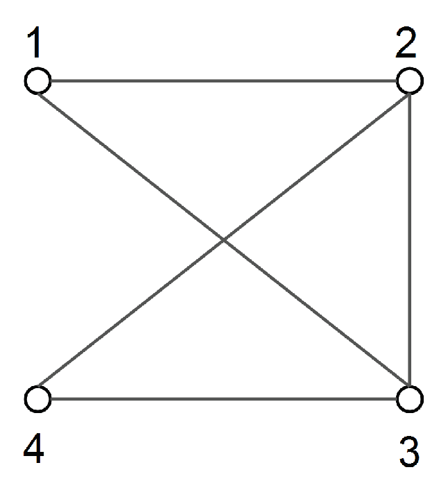
2.1. Graph Theory
2.2. Consensus Algorithm
3. Problem Formulation
3.1. Analytic Solution to EDP
3.1.1. Modeling
3.1.2. Solution
3.2. Fully Distributed Solution to EDP
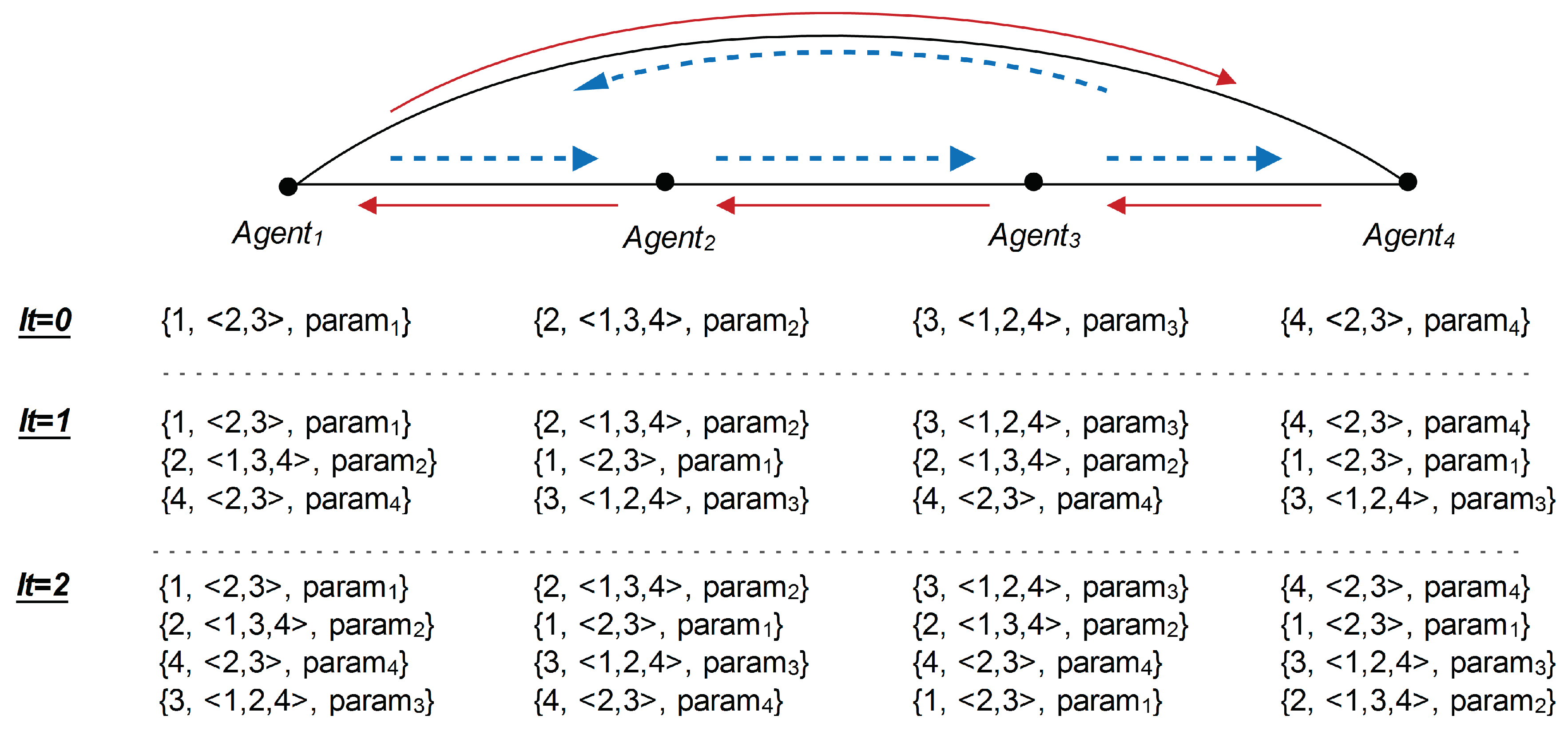
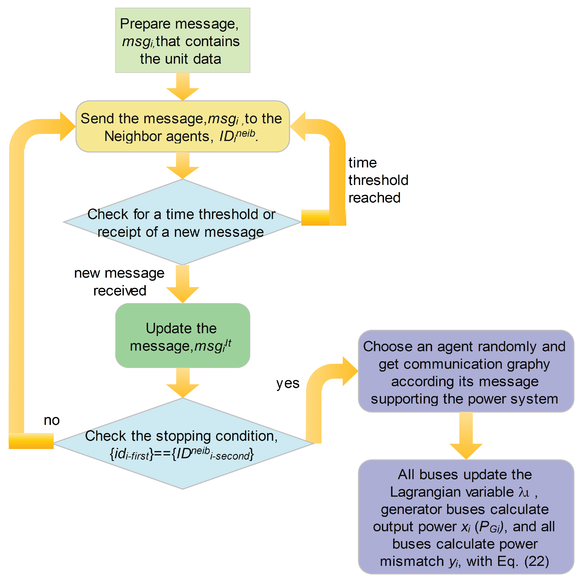
3.2.1. Data Collection
| Algorithm 1 Data Collection Algorithm Based on FBC |
|
3.2.2. -Consensus Algorithm
3.2.3. Algorithm Analysis
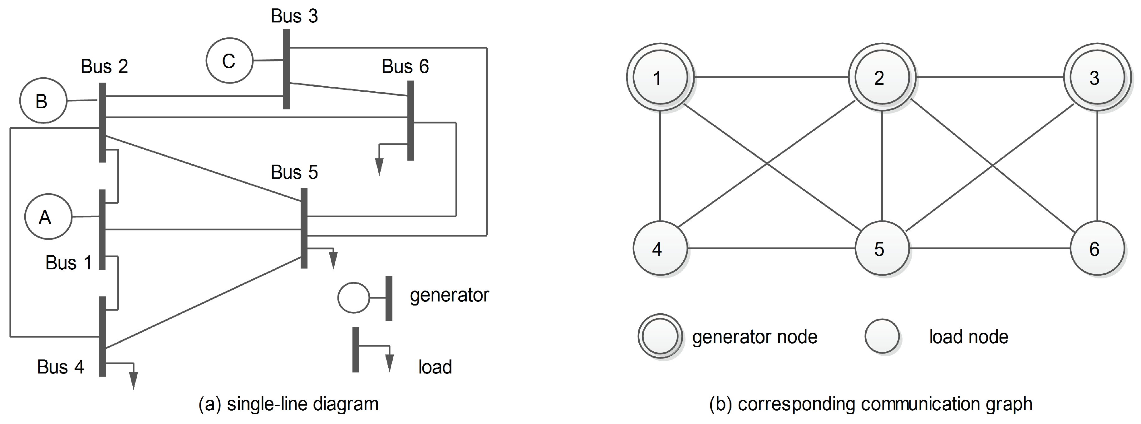
4. Simulation Results
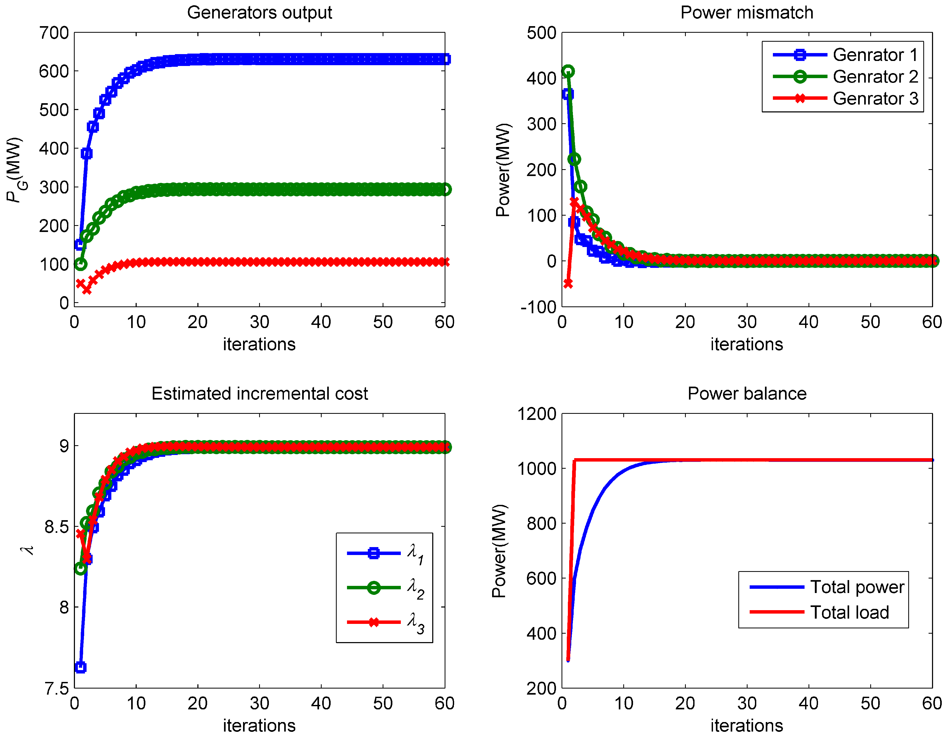
4.1. Case Study 1: Without Generator Constraints
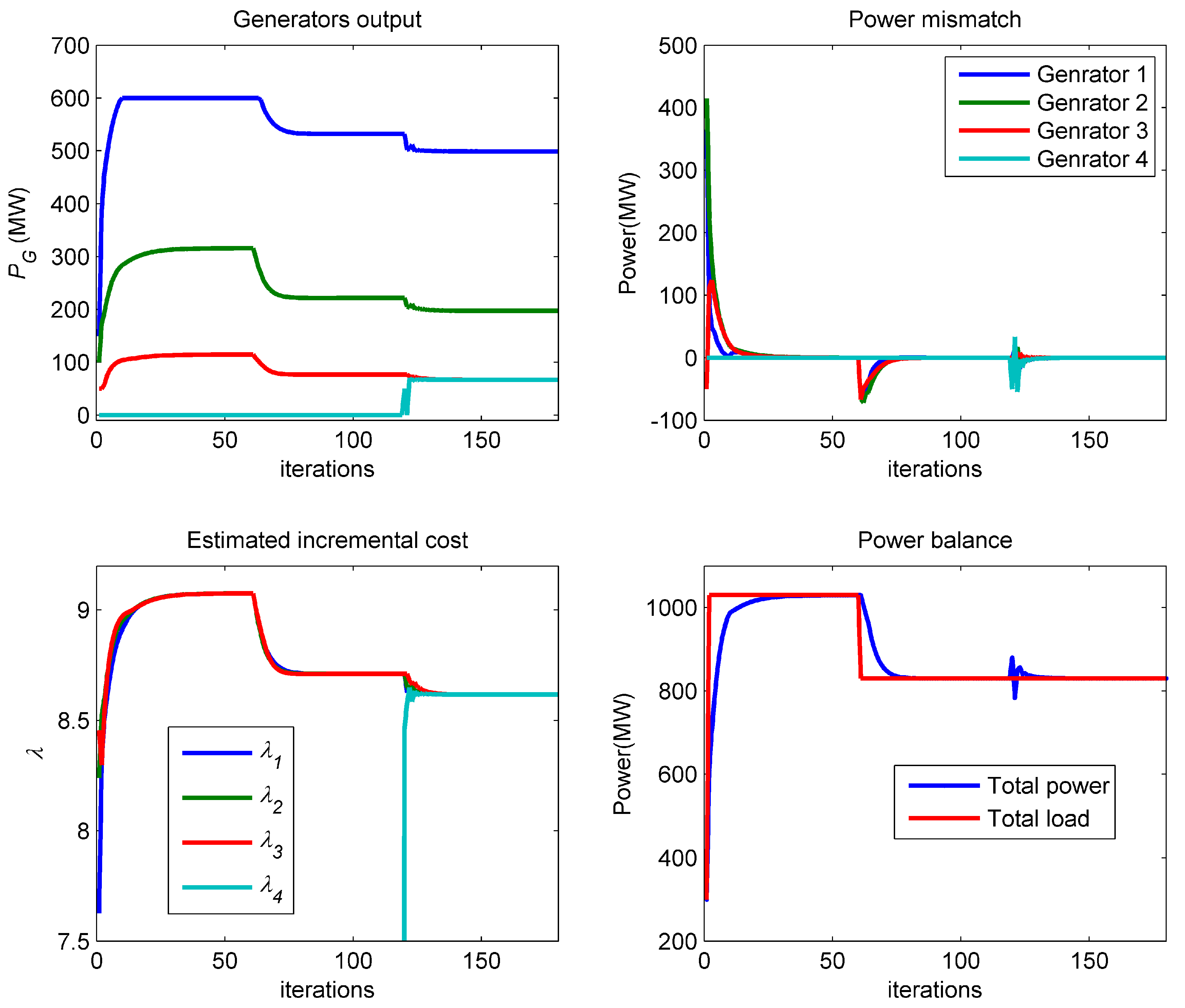
4.2. Case Study 2: With Generator Constraints
4.3. Case Study 3: Plug and Play Capability
4.4. Case Study 4: Implementation on IEEE 57-Bus System
5. Conclusions
Author Contributions
Funding
Acknowledgments
Conflicts of Interest
Abbreviations
| SG | Smart Grid |
| EDP | Economic Dispatch Problem |
| WAMSs | Wide Area Measurement Systems |
| SANETs | Sensor and Actuator Networks |
| WAN | Wide Area Network |
| NAN | Neighborhood Area Network |
| HAN | Home Area Network |
| MAS | Multi-Agent System |
| DCOPF | DC Optimal Power Flow |
| ID | Identifier |
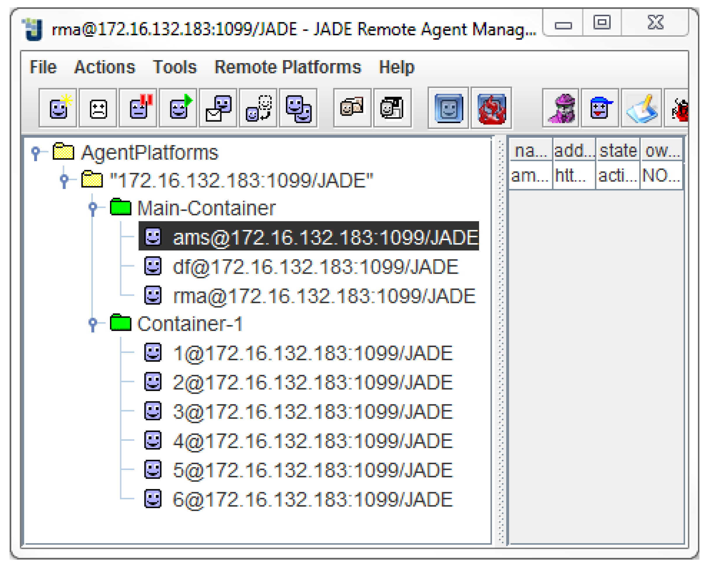
| JADE | Java Agent DEvelopment Framework |
| FBC | Flooding Based Consensus |
| In-neighbor set for node i | |
| Out-neighbor set for node i | |
| In-degree of node i | |
| Out-degree of node i | |
| The cardinality of a set | |
| Power generated by generator i | |
| Load demand in bus j | |
| Total load demand | |
| , , | Paraments about the cost of generator i |
| Maximum power generated by generator i | |
| Minimum power generated by generator i | |
| The holding message of agent i after iterations | |
| unique identifier of agent i | |
| Identifiers set about the neighbors of agent i Parameters of agent i or bus i |
References
- Fang, X.; Misra, S.; Xue, G.; Yang, D. Smart grid—The new improved power grid: A survey. IEEE Commun. Surv. Tutor. 2012, 14, 944–980. [Google Scholar] [CrossRef]
- Colak, I.; Sagiroglu, S.; Fulli, G.; Yesilbudak, M.; Covrig, C.F. A survey on the critical issues in smart grid technologies. Renew. Sustain. Energy Rev. 2016, 54, 396–405. [Google Scholar] [CrossRef]
- Kayastha, N.; Niyato, D.; Hossain, E.; Han, Z. Smart grid sensor data collection, communication, and networking: A tutorial. Wirel. Commun. Mob. Comput. 2014, 14, 1055–1087. [Google Scholar] [CrossRef]
- Hussain, H.M.; Javaid, N.; Iqbal, S.; Hasan, Q.; Aurangzeb, K.; Alhussein, M. An efficient demand side management system with a new optimized home energy management controller in smart grid. Energies 2018, 11, 190. [Google Scholar] [CrossRef]
- Caballero, V.; Vernet, D.; Zaballos, A.; Corral, G. Prototyping a web-of-energy architectrure for smart integration of sensor networks in smart grids domain. Sensors 2018, 18, 400. [Google Scholar] [CrossRef] [PubMed]
- European Technology Platform (ETP) SmartGrids. Strategic Deployment Document for Europe’s Electricity Networks of the Future. Available online: http://www.smartgrids.eu/documents/SmartGrids_SDD_FINAL_APPRIL2010.pdf (accessed on 2 June 2018).
- European Commission Research. European Smart Grida Technology Platform Vision and Strategy for Europe’s Electricity Networks of the Future. Available online: http://ec.europa.eu/research/energy/pdf/smartgrids_en.pdf (accessed on 2 June 2018).
- United States Department of Energy. The Smart Grid: An Introduction. Available online: http://www.oe.energy.gov/SmartGridIntroduction.htm (accessed on 2 June 2018).
- Uludag, S.; Lui, K.; Ren, W. Secure and scalable data collection with time minimization in the smart grid. IEEE Trans. Smart Grid 2016, 7, 43–54. [Google Scholar] [CrossRef]
- Naranjo, P.; Pooranian, Z.; Shojafar, M.; Conti, M.; Buyya, R. FOCAN: A fog-supported smart city network architecture for management of applications in the internet of everything environments. arXiv, 2017; arXiv:1710.01801. [Google Scholar]
- Gungor, V.C.; Lu, B.; Hancke, G.P. Opportunities and challenges of wireless sensor networks in smart grid. IEEE Trans. Ind. Electron. 2010, 57, 3557–3564. [Google Scholar] [CrossRef]
- Mohammadi, A.; Dehghani, M.J.; Ghazizadeh, E. Game theoretic spectrum allocation in femtocell networks for smart electric distribution grids. Energies 2018, 11, 1635. [Google Scholar] [CrossRef]
- Yang, S.; Tan, S.; Xu, J. Consensus based approach for economic dispatch problem in a smart grid. IEEE Trans. Power Syst. 2013, 28, 4416–4426. [Google Scholar] [CrossRef]
- Lin, C.E.; Viviani, G.L. Hierarchical economic idspatch for piecewise quadratic cost functions. IEEE Trans. Power Appar. Syst. 1984, PAS-103, 1170–1175. [Google Scholar] [CrossRef]
- Zhan, J.P.; Wu, Q.H.; Guo, C.X.; Zhou, X. Fast λ-iteration medthod for economic dispatch with prohibited operating zones. IEEE Trans. Power Syst. 2014, 29, 990–991. [Google Scholar] [CrossRef]
- Duvvuru, N.; Swarup, K.S. A hybrid interior point assisted differential evolution algorithm for economic dispatch. IEEE Trans. Power Syst. 2011, 26, 541–549. [Google Scholar] [CrossRef]
- Lin, W.M.; Chen, S.J. Bid-based dynamic economic dispatch with an efficient interior point algorithm. Int. J. Electr. Power Energy Syst. 2002, 24, 51–57. [Google Scholar] [CrossRef]
- Chiang, C.L. Amproved genetic algorithm for power economic dispatch of units with valve-point effects and multiple fuels. IEEE Trans. Power Syst. 2005, 20, 1690–1699. [Google Scholar] [CrossRef]
- Walters, D.C.; Sheble, G.B. Gentetic algorithm solution of economic dispatch with valve opint loading. IEEE Trans. Power Syst. 1993, 8, 1325–1332. [Google Scholar] [CrossRef]
- Park, J.B.; Lee, K.S.; Shin, J.R.; Shin, J.R.; Lee, W.Y. A particle swarm optimization for economic dispatch with nonsmooth cost functions. IEEE Trans. Power Syst. 2005, 20, 34–42. [Google Scholar] [CrossRef]
- Panigrahi, B.K.; Pandi, V.R.; Das, S. Adaptive particle swarm optimization approach for static and dynamic economic load dispatch. Energy Convers. Manag. 2008, 49, 1407–1415. [Google Scholar] [CrossRef]
- Qin, Q.; Cheng, S.; Chu, X.; Lei, X.; Shi, Y. Solving non-convex/non-smooth economic load dispatch problems via an enhanced particle swarm optimization. Appl. Soft Comput. 2017, 59, 229–242. [Google Scholar] [CrossRef]
- Neto, J.X.V.; Reynoso-Meza, G.; Ruppel, T.H.; Mariani, V.C.; Coelho, L.S. Solving non-smooth economic dispatch by a new combination of continuous GRASP algorithm and differential evolution. Electr. Power Energy Syst. 2017, 84, 13–24. [Google Scholar] [CrossRef]
- Noman, N.; Iba, H. Differential evolution for economic load diapatch problems. Electr. Power Syst. Res. 2008, 78, 1322–1331. [Google Scholar] [CrossRef]
- Nimma, K.S.; AI-Falahi, M.D.A.; Nguyen, H.D.; Jayasinghe, S.; Mahmoud, T.S.; Negnevitsky, M. Grey wolf optimization-based optimum energy-management and battery-sizing method for grid-connected microgrids. Energies 2018, 11, 847. [Google Scholar] [CrossRef]
- Kamboj, V.K.; Bhadoria, A.; Bath, S.K. Solution of non-convex economic load diaptch problem for small-scale power systems using ant lion optimizer. Neural Comput. Appl. 2017, 28, 2181–2192. [Google Scholar] [CrossRef]
- He, D.; Wang, M.; Wang, J.; Xu, D. Study on control strategy for synchronous grid-connection of micro-grid. J. Northeast Electr. Power Univ. 2017, 37, 21–27. [Google Scholar]
- Fallah, S.N.; Deo, R.C.; Shojafar, M.; Conti, M.; Shamshirband, S. Computational intelligence approaches for energy load forecasting in smart energy management grids: state of the art, future challenges, and research directions. Energies 2018, 11, 596. [Google Scholar] [CrossRef]
- Binetti, G.; Davoudi, A.; Lewis, F.L.; Naso, D.; Turchiano, B. Distributed consensus-based economic dispatch with transmission losses. IEEE Trans. Power Syst. 2014, 29, 1711–1720. [Google Scholar] [CrossRef]
- Binetti, G.; Davoudi, A.; Naso, D. A distributed auction-based algorithm for the nonconvex economic dispatch problem. IEEE Trans. Ind. Inform. 2014, 10, 1124–1132. [Google Scholar] [CrossRef]
- Li, F.; Qiao, W.; Sun, H.; Wan, H.; Wang, J.; Xia, Y.; Xu, Z.; Zhang, P. Smart transmission grid: vision and framework. IEEE Trans. Smart Grid 2010, 1, 168–177. [Google Scholar] [CrossRef]
- Kar, S.; Hug, G. Distributed robust economic dispatch in power systems: A consensus+ innovations approach. In Proceedings of the 2012 IEEE Power and Energy Society General Meeting, San Diego, CA, USA, 22–26 July 2012. [Google Scholar]
- Zhang, Z.; Chow, M. Convergence analysis of the incremental cost consensus algorithm under different communication network topologies in a smart grid. IEEE Trans. Power Syst. 2012, 27, 1761–1768. [Google Scholar] [CrossRef]
- Kouveliotis-Lysikatos, I.; Hatziargyriou, N. Fully distributed economic dispatch of distributed generators in active distribution networks considering losses. IET Gener. Transm. Distrib. 2017, 11, 627–636. [Google Scholar] [CrossRef]
- Xu, Y.; Li, Z. Distributed optimal resource management based on the consensus algorithm in a microgrid. IEEE Trans. Ind. Electron. 2015, 62, 2584–2592. [Google Scholar] [CrossRef]
- Pooranian, Z.; Abawajy, J.H.; Vinod, P.; Conti, M. Scheduling distributed energy resource operation and daily power consumption for a smart building to optimize economic and environmental parameters. Energies 2018, 11, 1348. [Google Scholar] [CrossRef]
- Elsayed, W.T.; EI-Saadany, E.F. A fully decentralized approach for solving the economic dispatch problem. IEEE Trans. Power Syst. 2015, 30, 2179–2189. [Google Scholar] [CrossRef]
- Pooranian, Z.; Nikmehr, N.; Najafi-Ravadanegh, S.; Mahdin, H.; Abawajy, J. Economical and environmental operation of smart networked microgrids under uncertainties using NSGA-II. In Proceedings of the 24th International Conference on Software, Telecommunications and Computer Networks (SoftCOM), Split, Croatia, 22–24 September 2016. [Google Scholar]
- Li, C.; Yu, X.; Yu, W.; Yu, W.; Huang, T.; Liu, Z.W. Distributed event-triggered scheme for economic dispatch in smart grids. IEEE Trans. Ind. Inform. 2016, 12, 1775–1785. [Google Scholar] [CrossRef]
- Xu, Y.; Sun, H.; Liu, H.; Liu, H.; Fu, Q. Distributed solution to DC optimal power flow with congestion management. IEEE Electr. Power Energy Syst. 2018, 95, 73–82. [Google Scholar] [CrossRef]
- Bondy, J.A.; Murty, U.S.R. Graph Theory with Applications; Elsevier: New York, NY, USA, 1976. [Google Scholar]
- Lin, Z.; Francis, B.; Maggiore, M. Distributed Control and Analysis of Coupled Cell Systems; VDM Verlag: Saarbrucken, Germany, 2008. [Google Scholar]
- DeGroot, M.H. Reaching a consensus. J. Am. Stat. Assoc. 1974, 69, 118–121. [Google Scholar] [CrossRef]
- Horn, R.A.; Johnson, C.R. Matrix Analysis, 2nd ed.; Cambridge University Press: New York, NY, USA, 2013. [Google Scholar]
- Wood, A.J.; Wollenberg, B.F. Power Generation, Operation, and Control; John Wiley & Sons: New York, NY, USA, 1984. [Google Scholar]
- Saligrama, V.; Alanyali, M. A token based approach to distributed computation in sensor networks. IEEE J. Sel. Top. Signal Process. 2011, 5, 817–832. [Google Scholar] [CrossRef]


| Generator Type | A | B | C |
|---|---|---|---|
| (MW) | [150, 600] | [100, 400] | [50, 200] |
| a ($/MWh) | 0.00142 | 0.00194 | 0.00482 |
| b ($/MWh) | 7.2 | 7.85 | 7.97 |
| c ($/h) | 510 | 310 | 78 |
| (MW) | |||
| (MWh) | 352.1 | 257.7 | 103.7 |
| Bus | a ($/MW2h) | b ($/MWh) | (MW) | (MW) |
|---|---|---|---|---|
| 1 | 0.078 | 20 | 0 | 575.88 |
| 2 | 0.01 | 40 | 0 | 100 |
| 3 | 0.25 | 20 | 0 | 140 |
| 6 | 0.01 | 40 | 0 | 100 |
| 8 | 0.022 | 20 | 0 | 550 |
| 9 | 0.01 | 40 | 0 | 100 |
| 12 | 0.003 | 20 | 0 | 410 |
© 2018 by the authors. Licensee MDPI, Basel, Switzerland. This article is an open access article distributed under the terms and conditions of the Creative Commons Attribution (CC BY) license (http://creativecommons.org/licenses/by/4.0/).
Share and Cite
Li, B.; Wang, Y.; Li, J.; Cao, S. A Fully Distributed Approach for Economic Dispatch Problem of Smart Grid. Energies 2018, 11, 1993. https://doi.org/10.3390/en11081993
Li B, Wang Y, Li J, Cao S. A Fully Distributed Approach for Economic Dispatch Problem of Smart Grid. Energies. 2018; 11(8):1993. https://doi.org/10.3390/en11081993
Chicago/Turabian StyleLi, Bo, Yudong Wang, Jian Li, and Shengxian Cao. 2018. "A Fully Distributed Approach for Economic Dispatch Problem of Smart Grid" Energies 11, no. 8: 1993. https://doi.org/10.3390/en11081993
APA StyleLi, B., Wang, Y., Li, J., & Cao, S. (2018). A Fully Distributed Approach for Economic Dispatch Problem of Smart Grid. Energies, 11(8), 1993. https://doi.org/10.3390/en11081993