Smoothly Transitive Fixed Frequency Hysteresis Current Control Based on Optimal Voltage Space Vector

Abstract

This paper proposes a smoothly transitive fixed frequency hysteresis current control (ST-FHCC) scheme applied to an active power filter (APF). First of all, a switching fixed frequency hysteresis current control (S-FHCC) is introduced, which is based on phase-to-phase decoupling and switching the control strategies under mode 0 or mode 1, and its weakness is described in detail. To enhance it, an improved approach of regulating the hysteresis bandwidth is presented to fix the switching frequency with switch phases being regulated, based on the optimal voltage space vector (OVSV). Furthermore, a flexible division of the voltage-space-vectors diagram is developed to divide the original voltage-space-vectors diagram into six sub-regions, upon which the control strategies under mode 0 and mode 1 can be switched alternately in order to obtain a smooth transition. As a consequence, ST-FHCC can thoroughly avoid the inherent weakness of S-FHCC of switching that is not smooth as a result of the low control accuracy of current errors. Case studies are carried out through power systems computer aided design/electromagnetic transients including DC (PSCAD/EMTDC) while simulation results verify the effectiveness and superiority of ST-FHCC compared to S-FHCC.

1. Introduction

In the past decade, distributed generation (DG), including wind, hydro, solar, biomass, geothermal, tidal, fuel cell, has been widely deployed which can provide a powerful solution for the growing energy crisis resulting from the use of conventional fossil fuels, e.g., coal, gas, oil [1,2,3,4,5,6,7,8]. The integration of large-scale DG into the power grid will inevitably degrade power quality [9,10,11], in which harmonics due to adoption of converters of DG have a severe impact on the devices connected to the power system, which has gained enormous attention in recent year [12,13]. At present, the active power filter (APF) is one of the most effective tools for harmonics reduction [14], which usually adopts hysteresis current control (HCC) to realize an efficient harmonics compensation thanks to its elegant merits of simple implementation, high accuracy and fast response [15].

Generally speaking, there are two types of HCC: fixed bandwidth HCC (BHCC) and fixed frequency HCC (FHCC). Here, the fluctuation of switching frequency of BHCC often causes an unfavorable increase of switching losses, which will result in considerable noise and a difficulty in filter design [16,17,18]. To handle the above issue, FHCC has been developed to fully suppress the fluctuation of switching frequency via an accurate bandwidth regulation [19,20]. Hence, FHCC has become a major technique for the current control of various power system devices, e.g., an uninterruptible power supply (UPS), motor, converter, APF, etc.

So far, an enormous variety of control schemes for FHCC has been designed. In [21], an FHCC without bandwidth was reported with the features of simple control, easy implementation in a digital way, robustness to the filter inductor, and excellent steady and dynamic performance, in which the hysteresis band is cancelled, and the switching frequency is fixed by adjusting online the sampling period while accurate system parameters are required. By comparison, [21,22] presented a constant-frequency hysteresis current control without a hysteresis bandwidth for a grid-connected voltage source inverter with the concept of formulating the switching function for dictating the switching times of the switches in the inverter within a predefined switching period by predicting the current reference, system dynamic behavior, and past time. The technique retains the benefit of the hysteresis control having fast dynamic response and tackles the drawback of the standard hysteresis control having variable switching frequency. In [23], a variable-bandwidth hysteresis-modulation sliding-mode control was presented to realize the pulse frequency modulation, which utilizes a direct hysteresis modulation sliding-mode controller to perform the pulse width modulation (PWM), and employs a quasi-indirect sliding-mode controller to control the bandwidth of the hysteresis modulation. By using this method, the control circuit is of low cost and is simple, together with satisfactory transient and steady responses. Besides, [24] employed a fuzzy logic controller to facilitate the discarding of uncertainty in the APF by incorporating an adaptive fuzzy hysteresis band, which has a quite simple structure and is relatively easy to implement in practice. Moreover, [25] proposed a constant hysteresis-band current controller with lower fixed switching frequency by adding a zero mode control at a proper time, such that the hysteresis bandwidth and switching frequency can be simultaneously fixed via the use of an extra k-band to create a degree of freedom. Furthermore, [26] proposed a current-error space-vector-based hysteresis controller with online boundary computation, which possesses the advantage that its phase voltage frequency spectrum is similar to that of a fixed switching frequency space vector pulse width modulated (SVPWM) inverter. In [27], the switching frequency control process was further improved by fine tuning the hysteresis bandwidth variations, such that the zero crossings of the phase-leg current errors could be synchronized with a fixed reference clock to achieve a nearest space vector switching sequence, as well as to ensure an optimal switched output spectrum. In addition, [28] devised a mixed-signal hysteretic current controller with the digital voltage-loop and the analog current-loop, such that a robust stability and parameter-insensitive current ripple were achieved by asynchronous error-voltage sampling, together with a fixed switching frequency via the real-time bandwidth adaptation. Besides, in [29], a new fixed frequency space-vector hysteresis-band current control was presented to maintain the switching frequency constant through the voltage vectors associated with the estimated outer hysteresis-band, which not only retains most benefits of BHCC but also offers a fixed switching frequency and independent interphases. In particular, the author of this paper previously proposed a switching fixed frequency hysteresis current control (S-FHCC) based on an optimal voltage space vector (OVSV), which can increase the amplification gain of DC-link voltage with respect to the line currents of APF. It can also enhance the tracking accuracy of the current reference and decrease the power losses of the power electronic switches [30,31].

Nevertheless, the current error of the APF will exceed the limit when the voltage reference space vector crosses the boundary of the adjacent sub-regions, which generally produces a periodical surge of current error that often undesirably degrades the current tracking accuracy [30,31]. In order to overcome the above obstacle, this paper proposes a smoothly transitive fixed frequency hysteresis current control (ST-FHCC) scheme based on OVSV. Firstly, S-FHCC is introduced based on phase-to-phase decoupling and switching the control strategies under mode 0 or mode 1, which requires an inner and outer hysteresis comparator. One of its weakness is that the control strategies will be switched only if current errors exceed the limit of the outer hysteresis bandwidth. Then, an improved approach of regulating the hysteresis bandwidth is presented to fix the switching frequency with switch phases being regulated, based on OVSV. Furthermore, a flexible division of the voltage-space-vectors diagram is designed to divide the original region into six sub-regions. By adopting the flexible division, the control strategies under mode 0 and mode 1 can be switched alternately. Lastly, comprehensive case studies are undertaken to evaluate and compare the control performance of S-FHCC and ST-FHCC.

The original contribution and novelty of this paper can be summarized into the following three aspects:

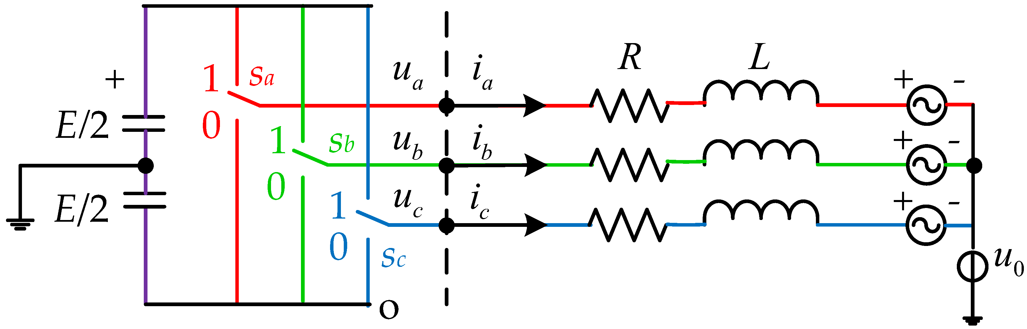
• The paper considers an APF in a three-phase-three-wire power system, in which FHCC is developed instead of the one given by [32,33,34]. Under such a configuration, the voltage between neutral point and dc-link midpoint of the APF results in a strong control coupling of three-phase, which has a dramatic impact on regulation of hysteresis bandwidth and fixed frequency. Hence phase-to-phase decoupling is implemented to eliminate the voltage, such that the two phase-to-phase current errors can be independently controlled by two switches with the third switch being a constant;
• Compared to [33,34], an improved approach of variable hysteresis bandwidth is presented in this paper, of which the midpoint of switch signals in the state of 0 is synchronized to the clock pulse with a constant frequency. Meanwhile, the equation is given to calculate the hysteresis bandwidth in the next period according to that in the current period. With this approach, fixed frequency and regulation of switch phases can be obtained simultaneously, such that the switching frequency can be constant while the uncontrollable phase-to-phase current error can be reduced greatly.
• A flexible division of the voltage-space-vector diagram is developed to divide the original voltage-space-vectors diagram into six sub-regions, upon which the control strategies under mode 0 and mode 1 can be switched alternately. As a result, a smooth transition can be realized while the inherent weakness of S-FHCC can be avoided, e.g., the control strategies will be switched only if current errors exceed the limit of the outer hysteresis bandwidth. The switching is far smoother with higher control accuracy and smaller current errors in ST-FHCC than those in S-FHCC.

The remainder of this paper is organized as follows: Section 2 aims to introduce the principle of S-FHCC. In Section 3, an approach of the variable hysteresis bandwidth is presented. ST-FHCC is described in detail in Section 4. Case studies are presented in Section 5 while some discussions about the results generated is given in Section 6. The work presented in the paper and some concluding remarks/findings are summarized in Section 7.

2. Switching Fixed Frequency Hysteresis Current Control (S-FHCC)

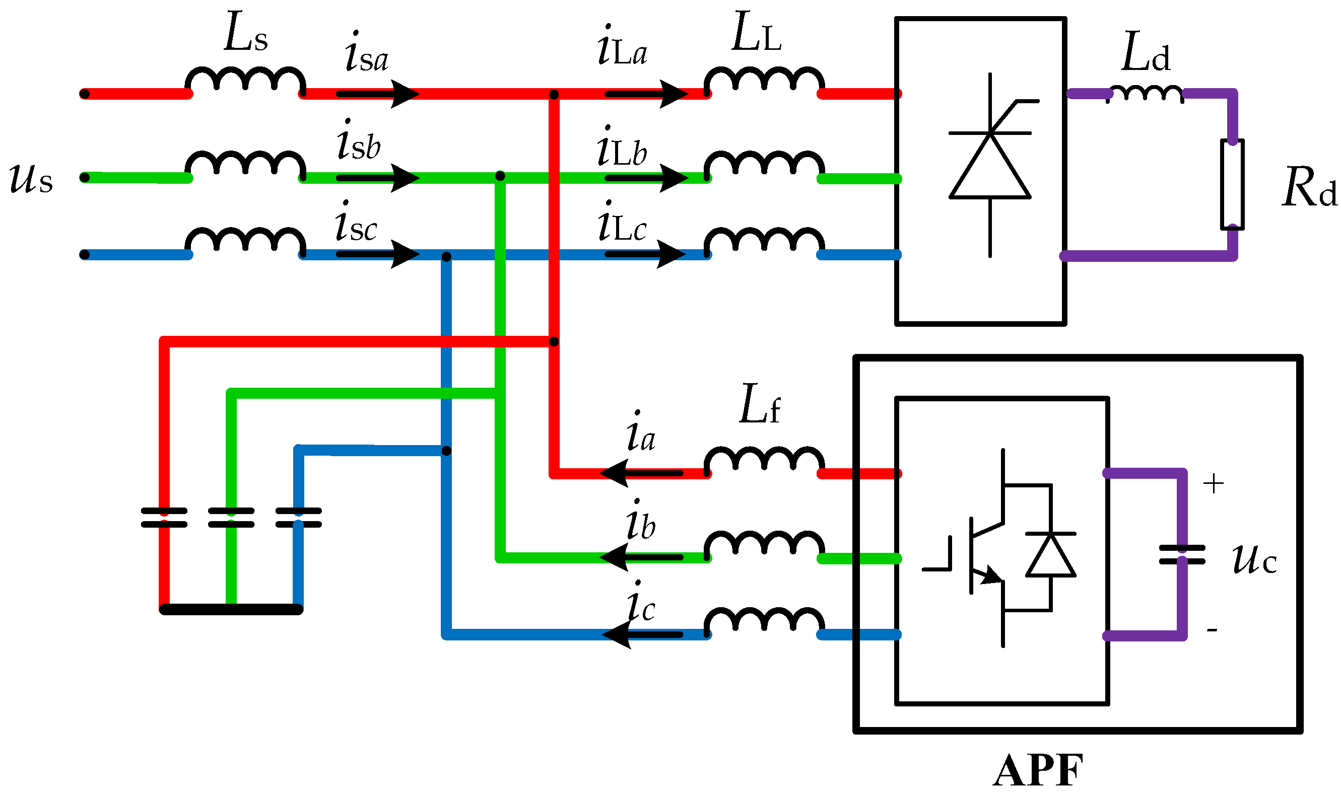
2.1. Active Power Filter (APF) Model

Figure 1 shows an equivalent circuit of a three-phase APF. Here, S_a, S_b and S_c represent three switching functions and 1 or 0 are used to represent their states, respectively. Here, 1 means the upper leg is turn-on and the lower leg is turn-off, while 0 means the opposite state. E is the DC-link capacitor voltage. R and L are resistor and inductor connected to the inverter bridge with the power grid. u₀ is the voltage between neutral point and ground. u_a, u_b, u_c are phase a, phase b and phase c terminal voltage with respect to the neutral point of inverter bridge O, while i_a, i_b i_c are phase a, phase b and phase c line currents, respectively.

The decoupling of phase-to-phase currents is required to obtain S-FHCC [30], such that the dynamics of current error can be written with a voltage-space-vector. Ignore the resistance, yields

$$L\frac{\mathrm{d}\Delta \mathit{i}}{\mathrm{d}t}={\mathit{u}}^{*}-\mathit{u}$$

(1)

where Δi is the difference between the line current space vector reference i^* and line current space vector i; u is a voltage-space-vector; and u^* is a voltage-space-vector reference corresponding to i^*, respectively. Expand (1) into

$$\{\begin{array}{c}L\frac{\mathrm{d}\Delta i_{ab}}{\mathrm{d}t}=u_{ab}^{*}-(S_a-S_b)\cdot E\\ L\frac{\mathrm{d}\Delta i_{bc}}{\mathrm{d}t}=u_{bc}^{*}-(S_b-S_c)\cdot E\\ L\frac{\mathrm{d}\Delta i_{ca}}{\mathrm{d}t}=u_{ca}^{*}-(S_c-S_a)\cdot E\end{array}$$

(2)

where $u_{ab}^{*}$,$u_{bc}^{*}$, $u_{ca}^{*}$ are the line voltage references of phase ab, phase bc, phase ca, respectively.

Δi_ab, Δi_bc, Δi_ca are given by

$$\begin{array}{l}\Delta i_{ab}=i_{ab}^{*}-i_{ab}\\ \Delta i_{bc}=i_{bc}^{*}-i_{bc}\\ \Delta i_{ca}=i_{ca}^{*}-i_{ca}\end{array}$$

(3)

where $i_{ab}^{*}$, $i_{bc}^{*}$, $i_{ca}^{*}$ are the phase-to-phase current references of phase ab, phase bc, phase ca, and i_ab, i_bc, i_ca are the differences between i_a and i_b, i_b and i_c, i_c and i_a, respectively.

From Equation (2), one can see that the phase-to-phase current errors are only determined by the corresponding two-phase switches, thus a decoupled current control could be realized. For instance, set S_b = 0 or 1 and Δi_ab and Δi_bc can be controlled by S_a and S_c, respectively. A similar control strategy can be derived when S_a or S_c are set to be a constant. Therefore, as shown in Figure 2, the voltage-space-vectors diagram can be divided into three parallelogram regions, each of which is denoted to be either mode 0 (one of the three switches S_a, S_b or S_c is fixed to be 0 while the others are arbitrary) or mode 1 (one of the three switches S_a, S_b or S_c is fixed to be 1 while the others are arbitrary).

The detailed control strategies under mode 0 and mode 1 in different parallelogram regions are given by

Table 1. Control strategies in different parallelogram regions under mode 0 and mode 1.

Regions	Mode 0			Regions	Mode 1
P01	Sa = 0	Sb controls Δiab	Sc controls Δica	P11	Sa = 1	Sb controls Δiab	Sc controls Δica
P02	Sb = 0	Sc controls Δibc	Sa controls Δiab.	P12	Sb = 1	Sc controls Δibc	Sa controls Δiab.
P03	Sc = 0	Sa controls Δica	Sb controls Δibc	P13	Sc = 1	Sa controls Δica	Sb controls Δibc

.

2.2. S-FHCC and Its Weakness

In literature [30,31], two hysteresis comparators employed in S-FHCC are depicted by Figure 3. The inner hysteresis comparator is adopted to detect whether the current error exceeds the inner bandwidth while the outer hysteresis comparator is used to detect whether the current error exceeds the outer bandwidth, which is larger than the inner bandwidth, such that the location of u^* could be determined.

In Figure 3, Sⁱ and S^e are logic vectors calculated by reversing the outputs of the inner hysteresis comparator and the outer hysteresis comparator while 2hⁱ and 2h^e are their hysteresis bandwidth, respectively. In addition, S represents the switching vector, given by

$$\begin{array}{l}{S}_a=S_{bc}^{\mathrm{e}}{\overline{S}}_{ca}^{\mathrm{e}}{\overline{S}}_{ca}^{\mathrm{i}}+S_{ab}^{\mathrm{e}}{\overline{S}}_{bc}^{\mathrm{e}}{S}_{ab}^{\mathrm{i}}\\ S_b=S_{ca}^{\mathrm{e}}{\overline{S}}_{ab}^{\mathrm{e}}{\overline{S}}_{ab}^{\mathrm{i}}+S_{bc}^{\mathrm{e}}{\overline{S}}_{ca}^{\mathrm{e}}{S}_{bc}^{\mathrm{i}}\\ S_c=S_{ab}^{\mathrm{e}}{\overline{S}}_{bc}^{\mathrm{e}}{\overline{S}}_{bc}^{\mathrm{i}}+S_{ca}^{\mathrm{e}}{\overline{S}}_{ab}^{\mathrm{e}}{S}_{ca}^{\mathrm{i}}\end{array}$$

(4)

Note that the location of u^* can be determined by the signs of the three line-to-line voltage references, i.e., $u_{ab}^{*}$,$u_{bc}^{*}$, $u_{ca}^{*}$, which is indicated by S^e. Besides, the phase lock aims at fixing the switching frequency of APF with a proportional-integral (PI) controller. More details of the S-FHCC can be found in references [30,31] for interested readers.

Nevertheless, an inherent weakness of S-FHCC is that the change of the location of u^* can be detected only if one of the three current errors exceeds the limit of the corresponding outer hysteresis bandwidth, such that the control strategy are changed. For instance, when u^* moves from region VI to region I shown by Figure 4a, the control strategy in region VI (S_c controls Δi_bc while S_a controls Δi_ab) is still adopted with the fact that Δi_bc will increase continuously despite the value of S_c until the current error Δi_bc exceeds the limit of the outer hysteresis comparator, as clearly provided in Figure 4b.

3. Fixed Swithcing Frequency Based on Optimal Voltage Space Vector (OVSV)

Since the uncontrollable current error is the negative sum of the other two phase-to-phase current errors under control, e.g., Δi_ab = −(Δi_bc + Δi_ca), Δi_bc and Δi_ca should be as close as possible in amplitude and opposite to each other in phase in order to decrease the amplitude of Δi_ab. Thus, the hysteresis bandwidth is required to fix switching frequency and to regulate the phase of two controllable switches. Moreover, an approach of fixing switching frequency with switch phases being regulated is presented such that the midpoint of switching signals in the state of 0 is synchronized to the clock pulse with a constant frequency, which is demonstrated as follows.

Assume u^* is in region P₀₂, shown in Figure 2. It can be seen that S_c and S_a can independently control Δi_bc and Δi_ab, respectively. u^* changes slightly during a switching period under high switching frequency, which could be ignored. Hence, the current error increases or decreases linearly with respect to time. The process of fixing the switching frequencies of S_a and S_c with switch phases being regulated are depicted in Figure 5, by which the current error will cross the zero-point of the clock pulse in each switching period. As a result, the switching frequencies of S_a and S_c remain constant, which is equal to that of the clock pulse. More importantly, the phases of S_a and S_c are regulated to be almost opposite.

According to Figure 5, in order to synchronize the clock pulse and the midpoint of the switch signals in the state of 0, the hysteresis bandwidths must satisfy:

$$(\frac{h_k}{2h_k/T_2}+\Delta t)+\frac{h_k+h_{k+1}}{2h_k/T_1}+\frac{h_{k+1}}{2h_k/T_2}=T_{\mathrm{s}}$$

(5)

where h_k and h_k+1 are the hysteresis bandwidth in the current switching period and in the next switching period; T₁ and T₂ denote the durations of the switch signal that stayed at 1 and 0 in the current switching period; T_s is a given switching period; and Δt is the difference between the midpoint of switch signal and clock pulse, respectively.

In S-FHCC, the adopted voltage-space-vectors are not optimal when the three-phase switches operate without regulating the phase of switches. In contrast, regulating the phase of switches cannot only decrease current error and harmonics, but can also lead to an OVSV.

For example, when u^* is in region I under mode 0, the waveforms of S_a, S_b, S_c and the sequence of voltage-space-vectors are (V₀, V₁, V₂, V₃, V₀) without regulating the phase of switches, as shown in Figure 6a. Moreover, this also demonstrates that the currents are controllable in the whole parallelogram region denoted by P₀₃. However, there are three OVSVs, i.e., V₀, V₁, V₂, and one suboptimal voltage-space-vector, i.e., V₃, in the adopted control set of voltage-space-vectors {V₀, V₁, V₂, V₃} [30,31], which cannot all be optimal.

With switch phases regulated, the waveforms of S_a, S_b, S_c and the operation sequence of voltage-space-vectors are (V₀, V₁, V₂, V₁, V₀), as shown in Figure 6b. Since region I belongs to the parallelogram region, the current error is also controllable in the region I. Furthermore, the adopted control set of voltage-space-vectors {V₀, V₁, V₂} is all optimal.

4. Smoothly Transitive Fixed-Frequency Hysteresis Current Control (ST-FHCC)

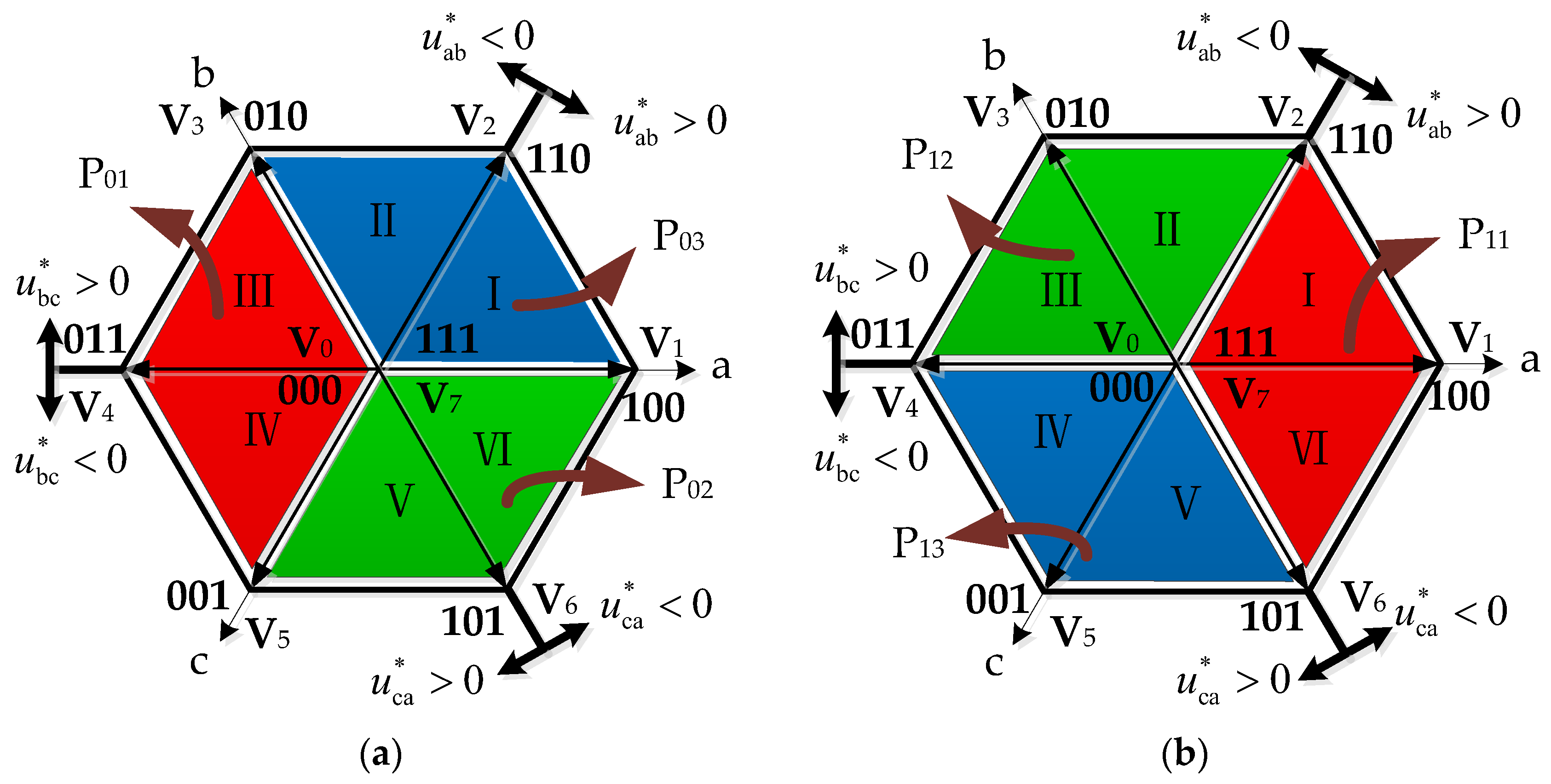
4.1. Flexible Division of Voltage-Space-Vector Diagram

To prevent the current error from exceeding its limit illustrated by Figure 4b, one should switch between mode 0 and mode 1. As shown in Figure 7a, the inherent weakness can be thoroughly overcome if the control strategy under mode 0 (S_b = 0, S_c → Δi_bc, S_a → Δi_ab) is switched into the control strategy under mode 1 (S_a = 1, S_b → Δi_ab, S_c → Δi_ca) before u^* crosses the boundary VI-I. Similarly, mode 1 should be switched into mode 0 before u^* crosses the boundary I-II. The reason is that in the overlapping area, two of the three current errors are always controllable, and the switching between mode 0 and mode 1 will not lead to what Figure 4b describes. Therefore, in order to smoothly transit the boundaries of the three parallelogram regions under mode 0 or mode 1, the control strategies under mode 0 and mode 1 should be switched in the overlapping areas of the two parallelogram regions under mode 0 and mode 1, respectively.

More specifically, before u^* crosses the boundary VI-I, mode 0 is switched into mode 1. Moreover, when u^* crosses the boundary VI-I, the operation sequence of voltage-space-vectors varies from S₁₆ to S₁₁, where S₁₆ and S₁₁ represent the operation sequences of (V₇, V₆, V₁, V₆, V₇) and (V₇, V₂, V₁, V₂, V₇), respectively. With u^* crossing the boundary VI-I, the duration of S_b staying at 0 decreases gradually which is contrary to that of S_c staying at 0, such that a smooth transition of three-phase switches can be realized, as shown from Figure 7b.

Remark 1.

u^* can be composed according to volt-second balance when u^* is located in region VI, as

$${\mathit{u}}^{*}=\frac{{T^{\prime }}_7}{T_s}{\mathbf{V}}_7+\frac{{T^{\prime }}_6}{T_s}{\mathbf{V}}_6+\frac{{T^{\prime }}_1}{T_s}{\mathbf{V}}_1$$

(6)

where$T_0^{\prime }$is the duration of V₇;$T_6^{\prime }$denotes the duration of V₆while$T_1^{\prime }$denotes the duration of V₁; and T_s is the switching period.

With u^* crossing the boundary VI-I, $T_6^{\prime }$ will decrease while $T_1^{\prime }$ will increase, which show that the duty-cycle of S_b narrows gradually which is contrary to that of S_c in Figure 7b. Moreover, when u^* is just located in the boundary VI-I, T₁ is equals to 0, which shows that the duty-cycle of S_b is equal to that of S_c. After u^* crosses the boundary, u^* will be composed of

$${\mathit{u}}^{*}=\frac{{T^{\prime }}_7}{T_s}{\mathbf{V}}_7+\frac{T_2{}^{\prime }}{T_s}{\mathbf{V}}_2+\frac{{T^{\prime }}_1}{T_s}{\mathbf{V}}_1$$

(7)

where $T_2^{\prime }$ is the duration of V₂.

With u^* changing continuously, $T_2^{\prime }$ will increase while $T_1^{\prime }$ will decrease, which illustrates that the duty-cycle of S_b decrease further which is contrary to that of S_c in Figure 7b.

The three parallelogram regions under mode 0 and those under mode 1 can produce six overlapping areas, i.e., I-VI, as depicted in Figure 2. The control strategies under mode 0 (mode 1) should be switched into those under mode 1 (mode 0) in these overlapping areas, for two controllable current errors are always under control by two switches in these overlapping areas. Hence, a switching boundary needs to be set in each overlapping area in order to switch between the control strategies under mode 0 and those under mode 1 in the overlapping areas. On the one hand, the voltage-space-vectors diagram can be divided into six symmetric sub-regions, e.g., A to F, in Figure 8a. Two different control modes are adopted to two adjacent sub-regions. The regions A, C and E are controlled by mode 1 while regions B, D and E are controlled by mode 0. Under such a scenario, the current error will not exceed its limit in the division boundaries. Besides, symmetrical division can offer a fast and accurate regulation of hysteresis bandwidth and phase. The detailed control strategies are tabulated in

Table 2. The detailed control strategies based on the flexible division.

Sub-Regions	Control Strategy
A	Sa = 1	Sb controls Δiab	Sc controls Δica
B	Sc = 0	Sa controls Δica	Sb controls Δibc
C	Sb = 1	Sa controls Δiab	Sc controls Δibc
D	Sa = 0	Sb controls Δiab	Sc controls Δica
E	Sc = 1	Sa controls Δica	Sb controls Δibc
F	Sb = 0	Sa controls Δiab	Sc controls Δibc

.

On the other hand, the voltage-space-vectors diagram can also be divided more flexibly and even asymmetrically in ST-FHCC, as illustrated by Figure 8b. Note that such a division provides more margins for switching control strategies, which is due to the fact that even if there is a slight estimation error of u^*, the current errors are still under control.

4.2. Switching of the Control Strategies in S-FHCC

As illustrated in Figure 9a, the operation sequence of voltage-space-vectors varies from S₀₆ to S₀₁ with u^* crossing from region VI to I, where S₀₆ and S₀₁ denote the operation sequences of (V₀, V₁, V₆, V₁, V₀) and (V₀, V₁, V₂, V₁, V₀), respectively. In S₀₆ or S₀₁, u will be V₀, V₁, V₆, V₁, V₀ or V₀, V₁, V₂, V₁, V₀ in sequence in a switching period. Consider that u^* is approximated to be a constant in a switching period, the derivatives of Δi with respect to the time are obtained from Equation (1) and depicted in Figure 9b, where (dΔi₁/dt), (dΔi₂/dt), (dΔi₃/dt) are the derivatives of Δi with respect to the time with u equal to V₀, V₁, V₆, respectively. Assume the initial Δi is zero to simplify the analysis. Δi will change in the directions of the derivatives of Δi with respect to the time in sequence. There are trajectories of Δi in a solid line and in a dotted line corresponding with S₀₆ and S₀₁, as clearly shown by Figure 9c. Moreover, the trajectories of Δi will gradually change from S₀₆ into S₀₁ with u^* changing.

In order to achieve a smooth switching of current error, the ideal switching point should be the zero-crossing of current errors according to Figure 9c, such that three-phase switches can switch smoothly.

Based on the above analysis, the switching point is determined by detecting whether current error exceeds the limit of the outer hysteresis bandwidth or not. In other words, the switching point cannot be selected as the zero-crossing point of current errors, which usually results in a low control accuracy and an unstable switching of three-phase switches that will affect the fixed-frequency control and regulation of the switches phase.

4.3. Smooth Switching of the Control Strategies in ST-FHCC

In ST-FHCC, when u^* crosses the division boundary, the switching time of each phase is used to determine the u^* location at first. Then, the zero-crossing point of current errors (according to the clock signal) is chosen as the switching point of mode 0 and mode 1 based on the u^* location and pre-divided voltage-space-vectors diagram, such that a smooth switching of current errors and three-phase switches can be realized.

For example, when u^* crosses from region A to B, the operation sequence of voltage-space-vectors varies from S₁₁ to S₀₁, where S₁₁ and S₀₁ denote the operation sequences of (V₇, V₂, V₁, V₂, V₇) and (V₀, V₁, V₂, V₁, V₀), respectively. The trajectories of current errors are depicted by Figure 10a, where α₀, α₁, α₂, α₇ are the derivatives of Δi with respect to time under the operations of V₀, V₁, V₂, V₇, respectively. The ideal switching point should be the zero-crossing point of current errors based on the clock signal in practice with the result that three-phase switches can switch smoothly, as shown in Figure 10b.

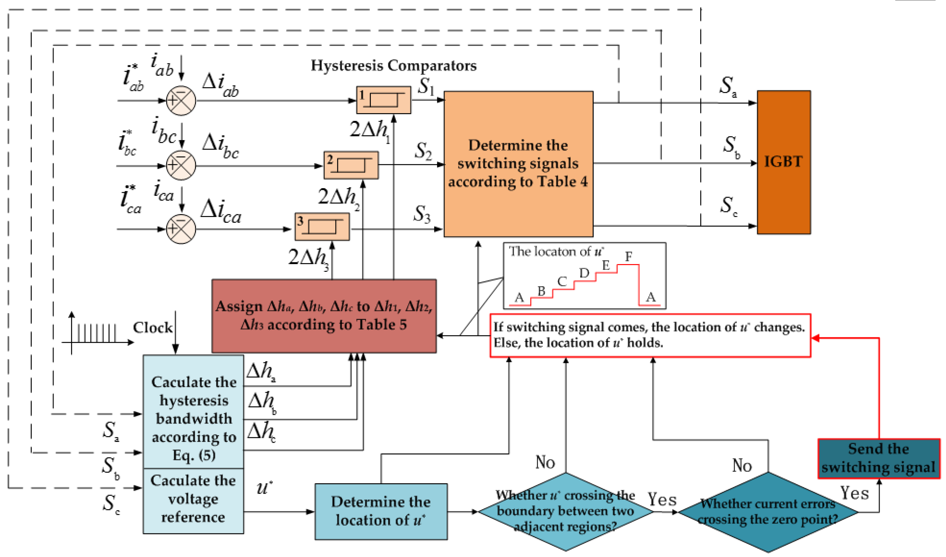
4.4. Detailed Procedure of ST-FHCC

The detail procedure of ST-FHCC is depicted by Figure 11. The three hysteresis comparators are set to output 0 when the current errors exceed their upper bandwidths while set to be 1 when the current errors exceed their lower bandwidths.

The following example illustrates the process of obtaining the ST-FHCC in detail.

When u^* is located in region A, S_a is fixed to be 1, and S_b controls Δi_ab while S_c controls Δi_ca. According to Equation (2), Δi_ab will increase when S_b stays at 1 while Δi_ab will decrease when S_b stays at 0. On the contrary, Δi_ca will decrease when S_c stays at 1 while Δi_ab will increase when S_c stays at 0. If the hysteresis comparator 1 outputs 1, it means that Δi_ab exceeds the lower bandwidth of the hysteresis comparator and needs to be increased. Thus, S₁ should be assigned to S_b. Similarly, if the hysteresis comparator 3 outputs 1, it means that Δi_ca exceeds the lower bandwidth of the hysteresis comparator and needs to be increased. Thus, $\overline{S_3}$ should be assigned to S_c. Consequently,

Table 3. The relationship between S₁, S₂, S₃ and S_a, S_b, S_c.

The Location of u*	A	B	C	D	E	F
The relationships	Sa = 1	Sa = $\overline{S_3}$	Sa = S1	Sa = 0	Sa = $\overline{S_3}$	Sa = S1
	Sb = $\overline{S_1}$	Sb = S2	Sb = 1	Sb = $\overline{S_1}$	Sb = S2	Sb = 0
	Sc = S3	Sc = 0	Sc = $\overline{S_2}$	Sc = S3	Sc = 1	Sc = $\overline{S_2}$

can be obtained.

According to S_a, S_b, and S_c, Δh_a, Δh_b, and Δh_c can be obtained by solving Equation (5), respectively. Since S_b controls Δi_ab while S_c controls Δi_ca, Δh_b should be the bandwidth of hysteresis comparator 1 to limit Δi_ab, such that Δh_b is assigned to Δh₁ while Δh_c should be the bandwidth of hysteresis comparator 3 to limit Δi_ca, such that Δh_c is assigned to Δh₃. Therefore,

Table 4. The relationship between Δh_a, Δh_b, Δh_c and Δh₁, Δh₂, Δh₃.

The Location of u*	A or D	B or E	C or F
The relationships	Δh1 = Δhb	Δh1 = *	Δh1 = Δha
	Δh2 = *	Δh2 = Δhb	Δh2 = Δhc
	Δh3 = Δhc	Δh3 = Δha	Δh3 = *

‘*’ means the hysteresis bandwidth can be set to an arbitrary constant.

can be obtained.

Remark 2.

The outer hysteresis comparator employed in S-FHCC is no longer required in ST-FHCC. The control strategy under mode 0 (mode 1) is switched into that under mode 1 (mode 0) in the overlapping areas produced by the parallelogram regions of mode 0 and those of mode 1, as two controllable current errors are always under control by two switches in the overlapping areas. Therefore, the current errors will not exceed the larger bandwidth of the outer hysteresis comparator with the switching procedures of ST-FHCC implemented. Furthermore, the outer hysteresis comparator is no longer required to switch the control strategies in ST-FHCC.

5. Case Studies

The effectiveness of ST-FHCC is evaluated and compared with that of S-FHCC [30] by power systems computer aided design/electromagnetic transients including DC (PSCAD/EMTDC). The test system is given by Figure 12, in which the APF is used to compensate the harmonic currents produced by the rectifier and the DC motor, while the system parameters are given as L_s = 0.001 H, L_L = 0.003 H, L_f = 0.0125 H, R_d = 37 Ω, L_d = 0.015 H, u_c = 800 V. The root-mean-square (RMS) of phase-to-phase voltage u_s is 380 V and the switching frequency of APF is 10 kHz. In addition, i_a, i_b, i_c are the line currents of APF; i_La, i_Lb, i_Lc are the line currents of the non-linear load; i_sa, i_sb, i_sc denote the line currents supplied by the three-phase power grid, respectively.

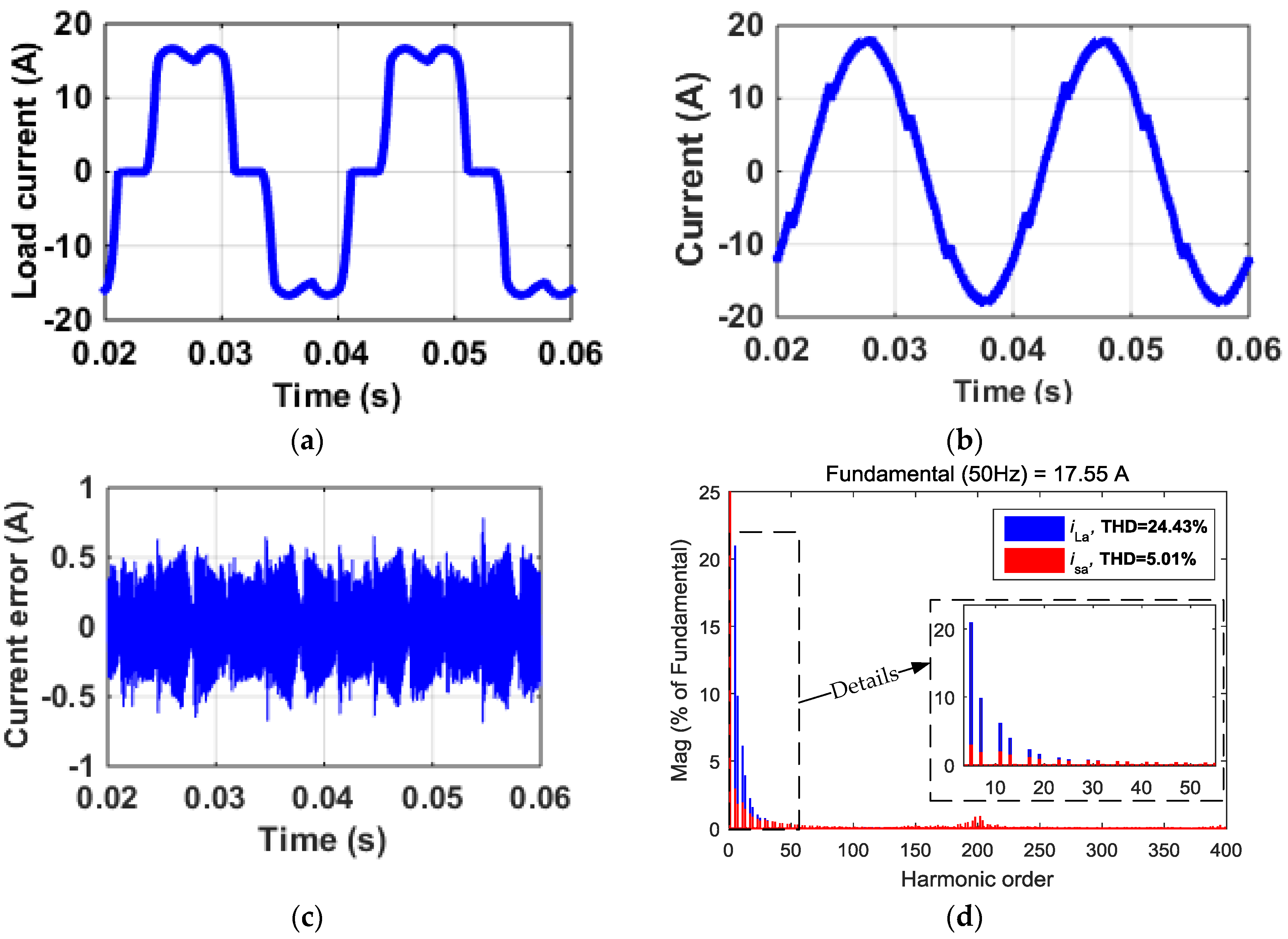
5.1. The Effect of Harmonics Compensation in ST-FHCC

Figure 13a,b show the load current of phase a and the system current of ST-FHCC after the harmonics compensation, which demonstrate that the harmonic current produced by the load can be effectively compensated. Moreover, Figure 13c illustrates that the current error of phase a is under control which is bounded between −0.8 A to 0.8 A. Figure 13d shows that the total harmonic distortion (THD) value of i_sa is reduced dramatically from 24.43 to 5.01% after i_sa is compensated by APF.

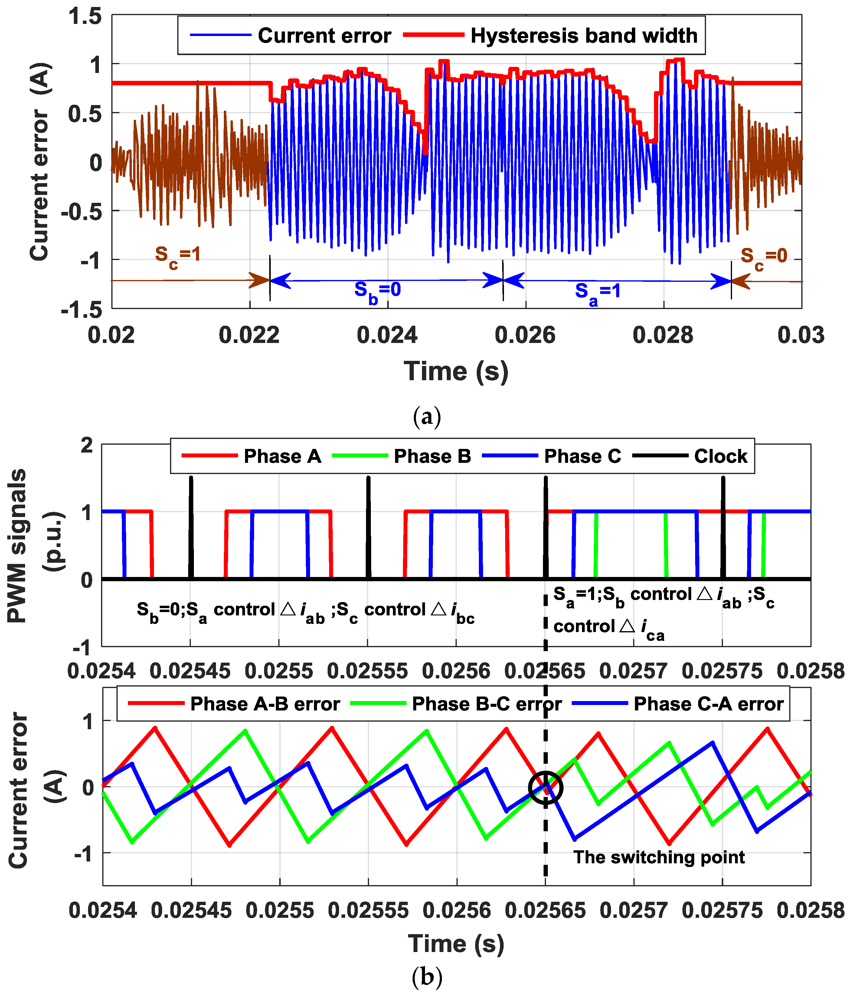
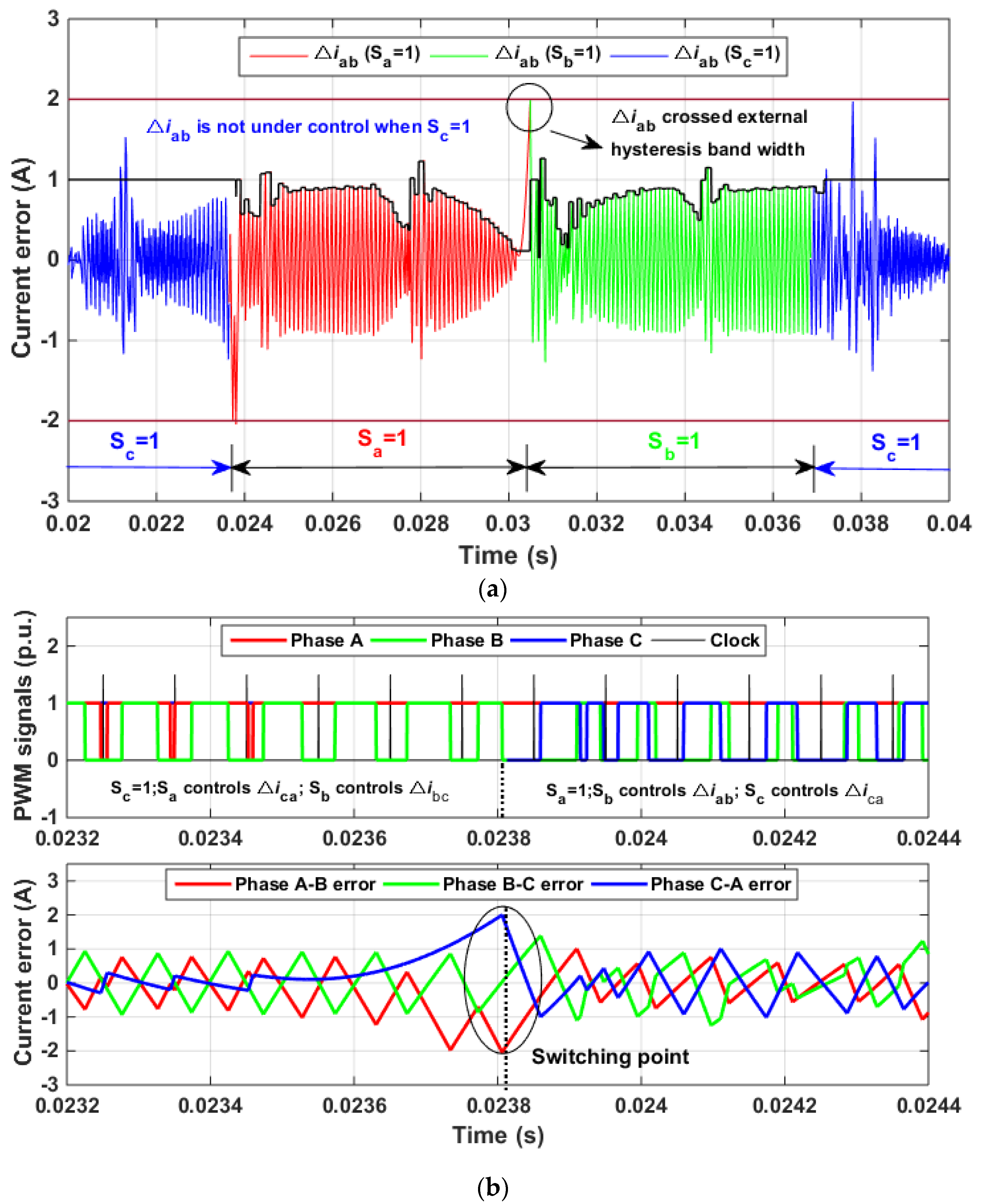
5.2. The Performance of the Current Errors in S-FHCC

The current error Δi_ab obtained by S-FHCC is given in Figure 14a, which shows that the control strategy is discontinuous with mode 1. When S-FHCC switches from S_a = 1 to S_b = 1, the phase-to-phase current error Δi_ab exceeds the limit, i.e., 2 A, of the outer hysteresis comparator. Here, Figure 14b enlarges the results obtained near 0.0238 s, in which it can be found that S-FHCC can only be switched after the current error exceeding the limit of the outer hysteresis comparator. During the switching, the transient process of current error phase and three-phase switches operation is disordered, which greatly affects the control of switching frequency and the switches phase.

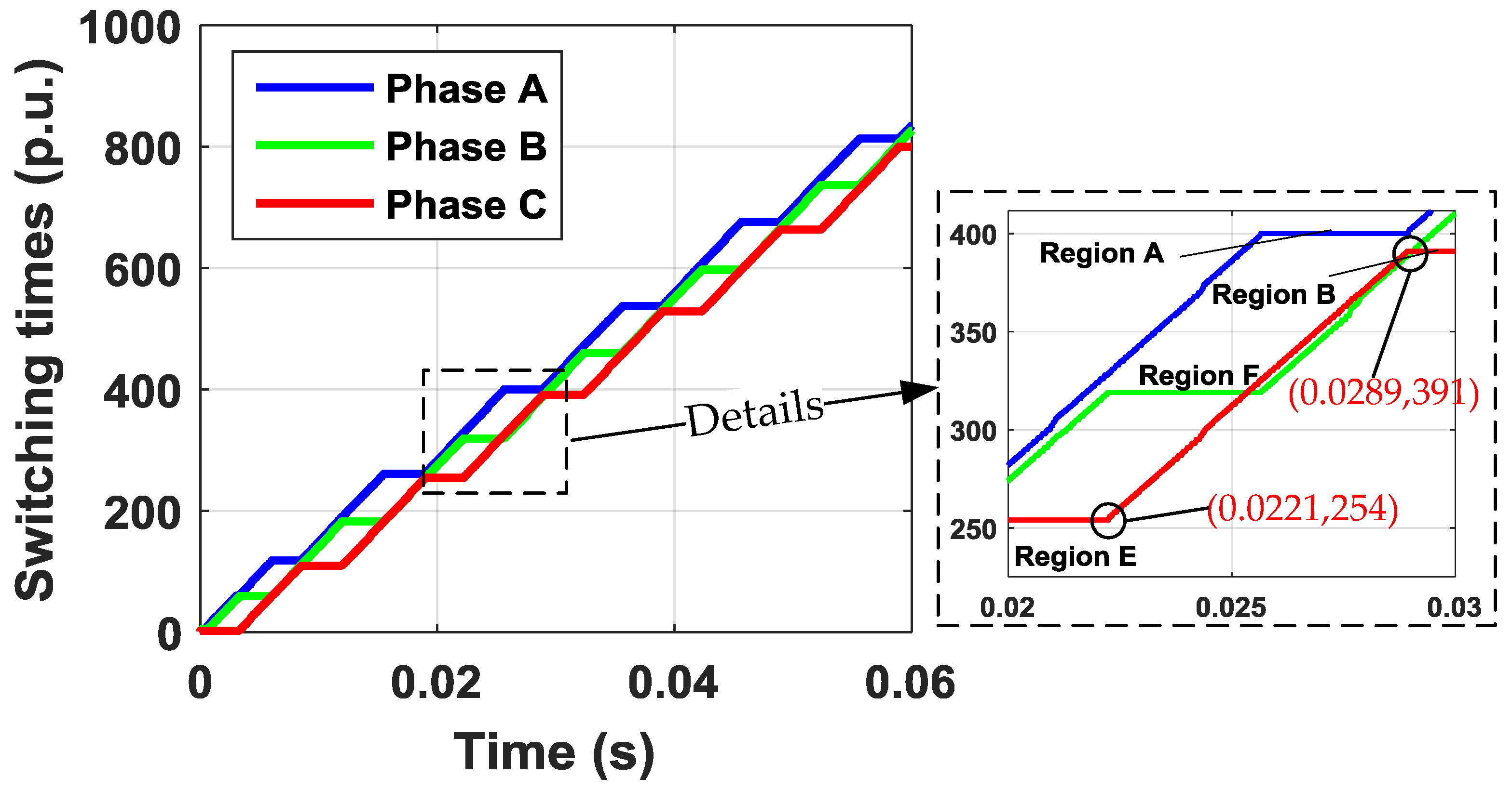
5.3. The Performance of the Current Errors in ST-FHCC

Figure 15a provides the changes of the phase-to-phase current error Δi_ab and the hysteresis bandwidth obtained during 0.02 s to 0.03 s, whose detailed variation is clearly shown by Figure 15b obtained during 0.0254 s to 0.0258 s.

From Figure 15a, one can observe that the current error Δi_ab is uncontrollable in region E (S_c = 1) and B (S_c = 0) while it becomes controllable in region F (S_b = 0) and A (S_a = 1), in which S_a controls Δi_ab in region F and S_b controls Δi_ab in region A. Meanwhile, Figure 15a shows that the hysteresis bandwidth is regulated continuously to fix the switching frequency in the region where Δi_ab is controllable.

From Figure 15b, it can be seen that the switching frequency is constant while the midpoint of two controllable switches in the state of 0 is synchronized to the clock signals, which results in an uncontrollable current error even to be smaller than that of the others. This is the reason that Δi_ca satisfies the equation: Δi_ca = −(Δi_ab + Δi_bc), and moreover, Δi_ab and Δi_bc are as close as possible in amplitude and opposite to each other in phase.

In particular, at the zero-crossing point of current errors near 0.02565 s, ST-FHCC switches from S_b = 0 (S_a controls Δi_ab and S_c controls Δi_bc) to S_a = 1 (S_b controls Δi_ab and S_c controls Δi_ca), which corresponds to the analysis of Table 2. Moreover, the current errors and operation of three-phase switches can change smoothly before and after the switching.

In addition, Figure 16 depicts the three-phase switching times by counting how three-phase switch signals rise and fall during 0 s–0.06 s. One of the three-phase switches does not operate in Region E, F, A and B, which is denoted by the horizontal straight lines. The operation times of the phase-C switch can be calculated as 20,147 times per second during 0.02 s–0.03 s. As shown by Figure 15b, the phase-C switch operates twice during a clock-pulse period due to the regulating phases of the switches. Therefore, the switching frequency is 10,073.5 Hz. Besides, the switching frequencies of the phase-A and the phase-C switches can be calculated as an approximate 10 kHz. Furthermore, the average switching frequencies of three-phase can be evaluated as an approximated 10 kHz even during 0 s–0.06 s. To summarize, the switching frequency can remain constant at 10 kHz by ST-FHCC.

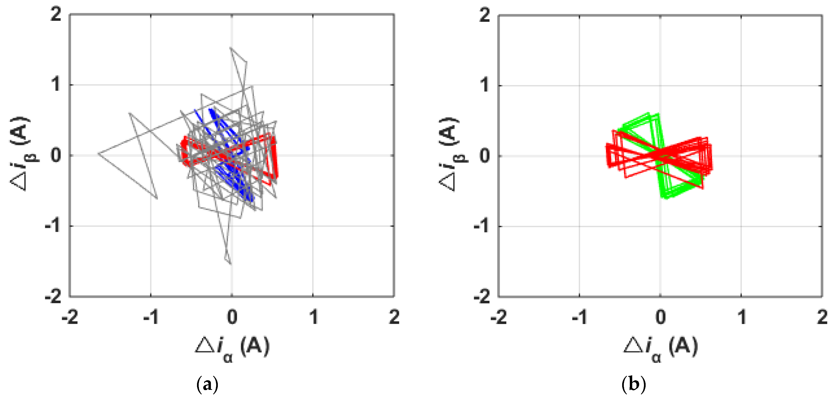
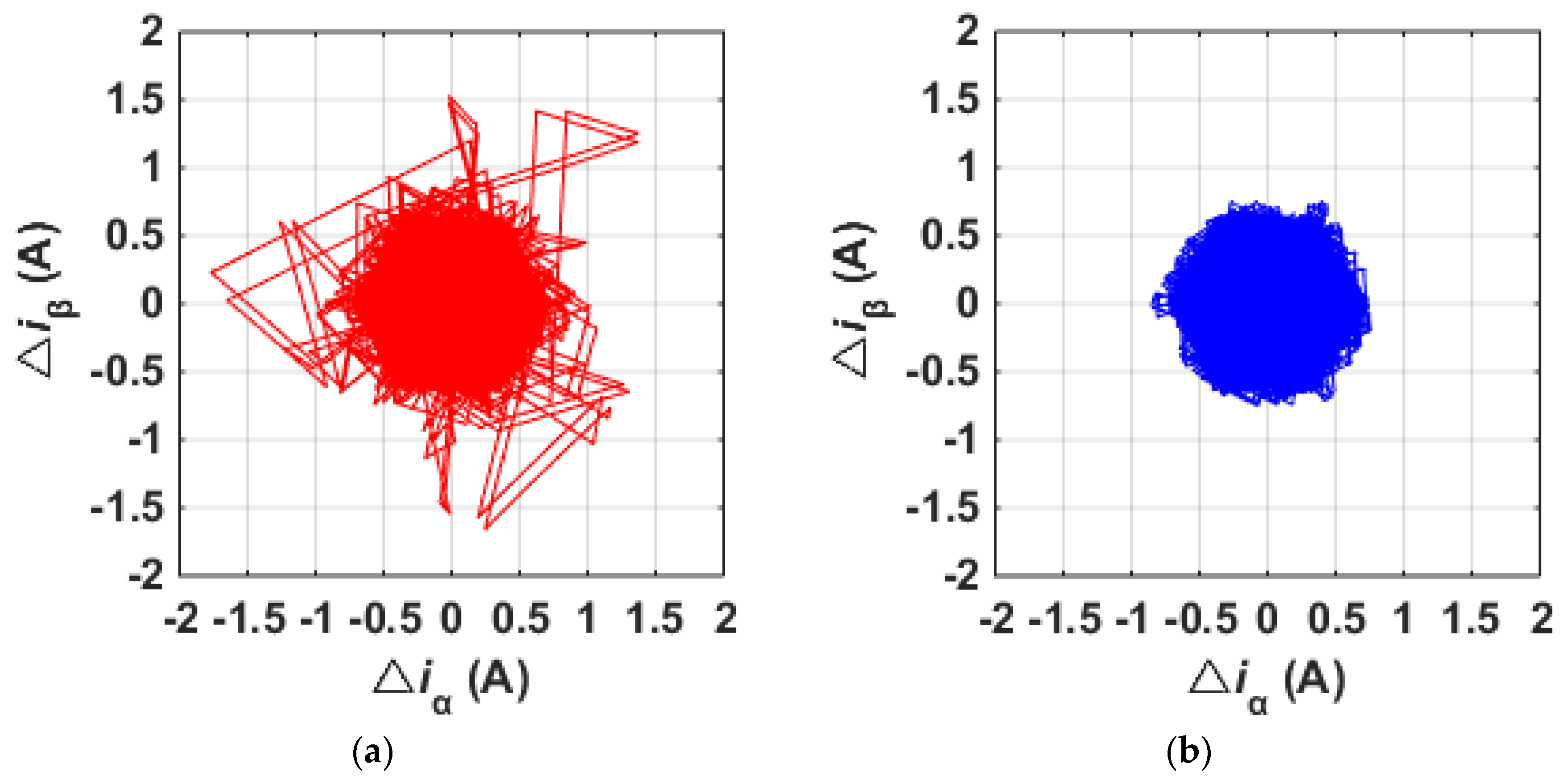
5.4. The Trajectories of Current Errors by S-FHCC and ST-FHCC

Figure 17a,b compares the switching trajectories of the current error space-vector of S-FHCC and ST-FHCC, respectively. One can see that ST-FHCC has no disorder of current error when switched at the zero-crossing point. In contrast, S-FHCC presents a significant disorder of current error when switched at the zero-crossing point.

Lastly, from Figure 18a,b, one can find that ST-FHCC can achieve a more stable and smoother current error compared to that of S-FHCC.

6. Discussions

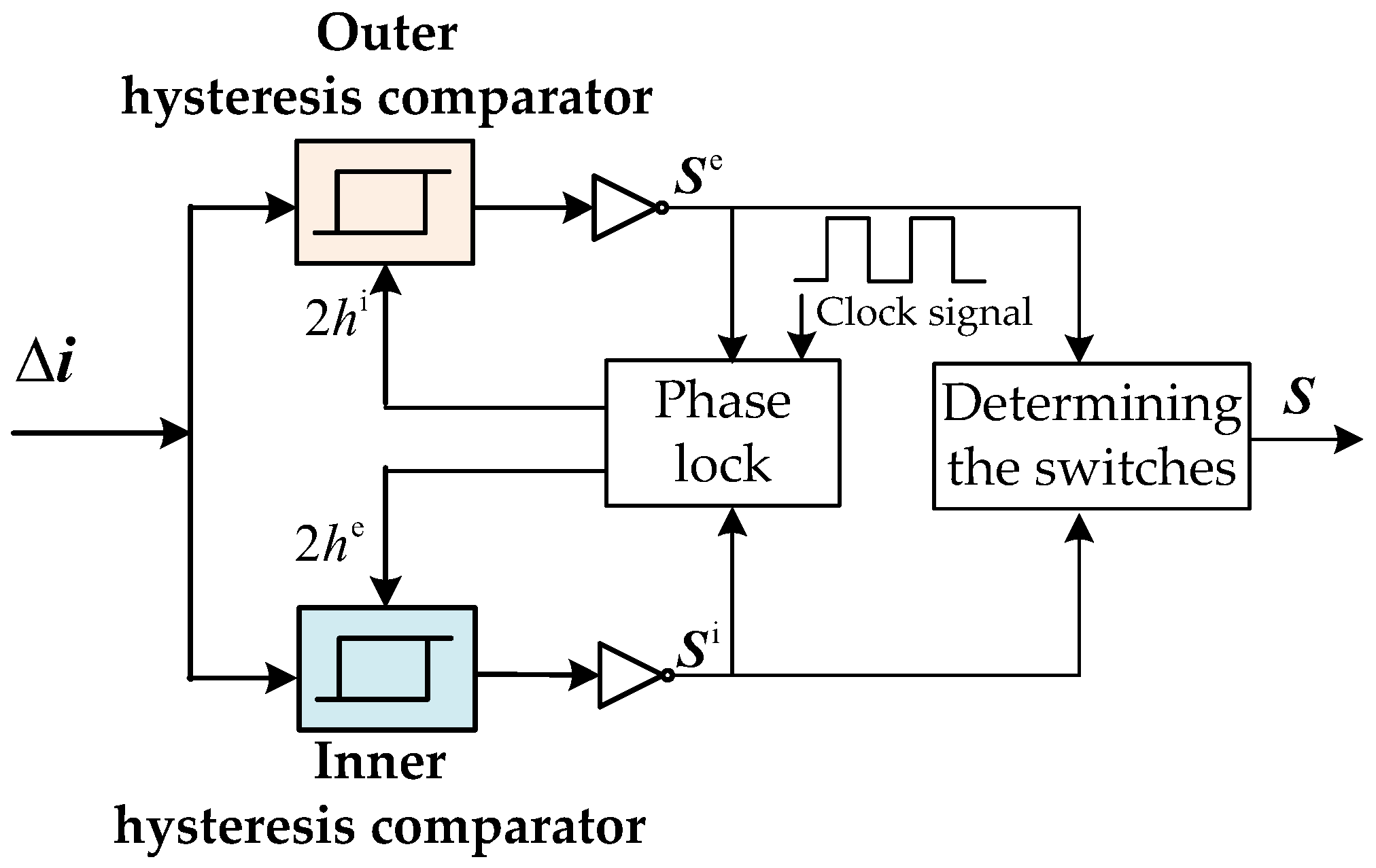
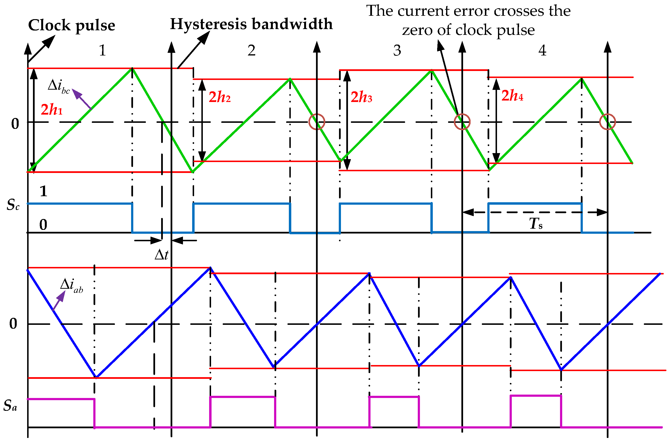
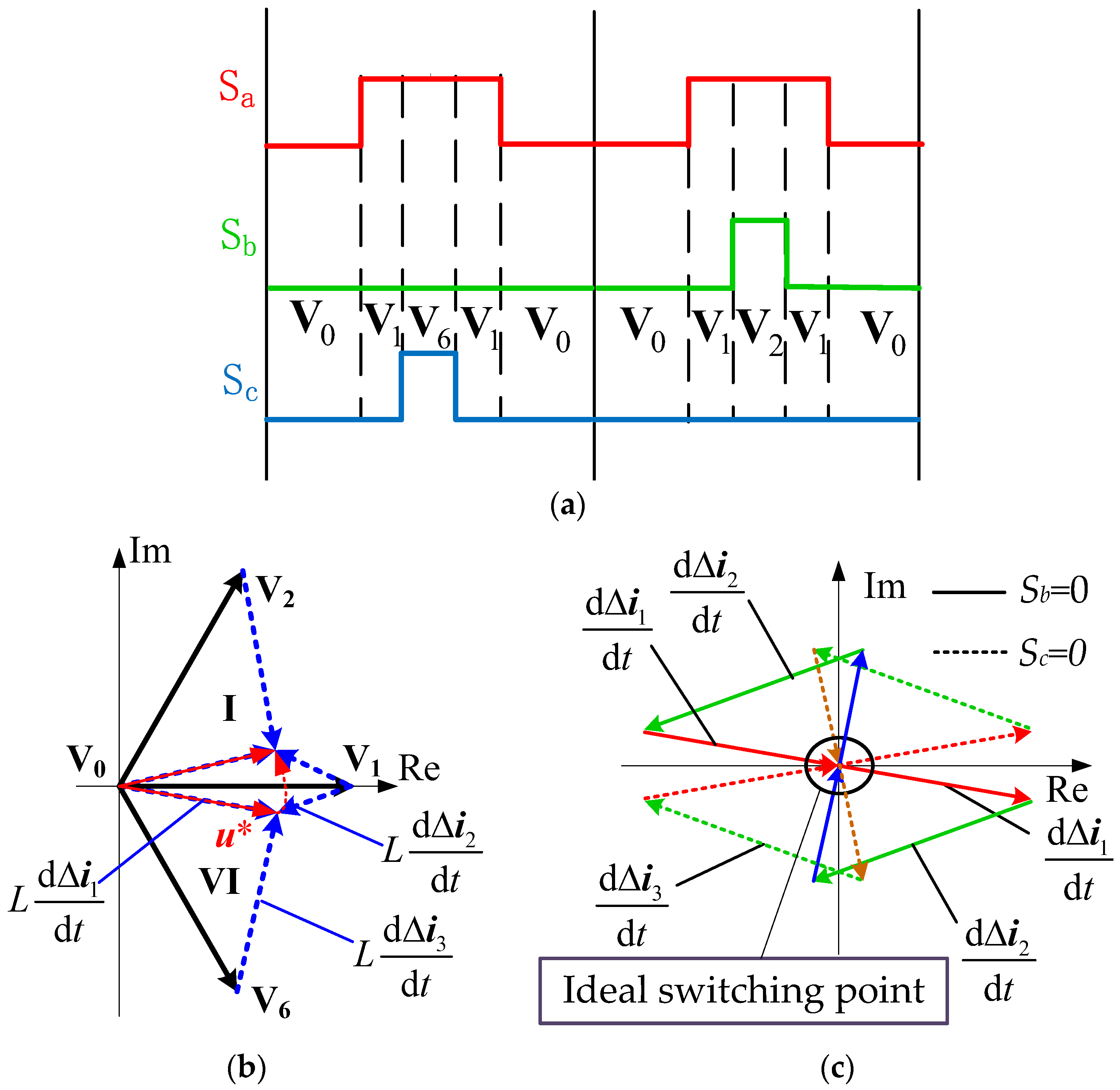
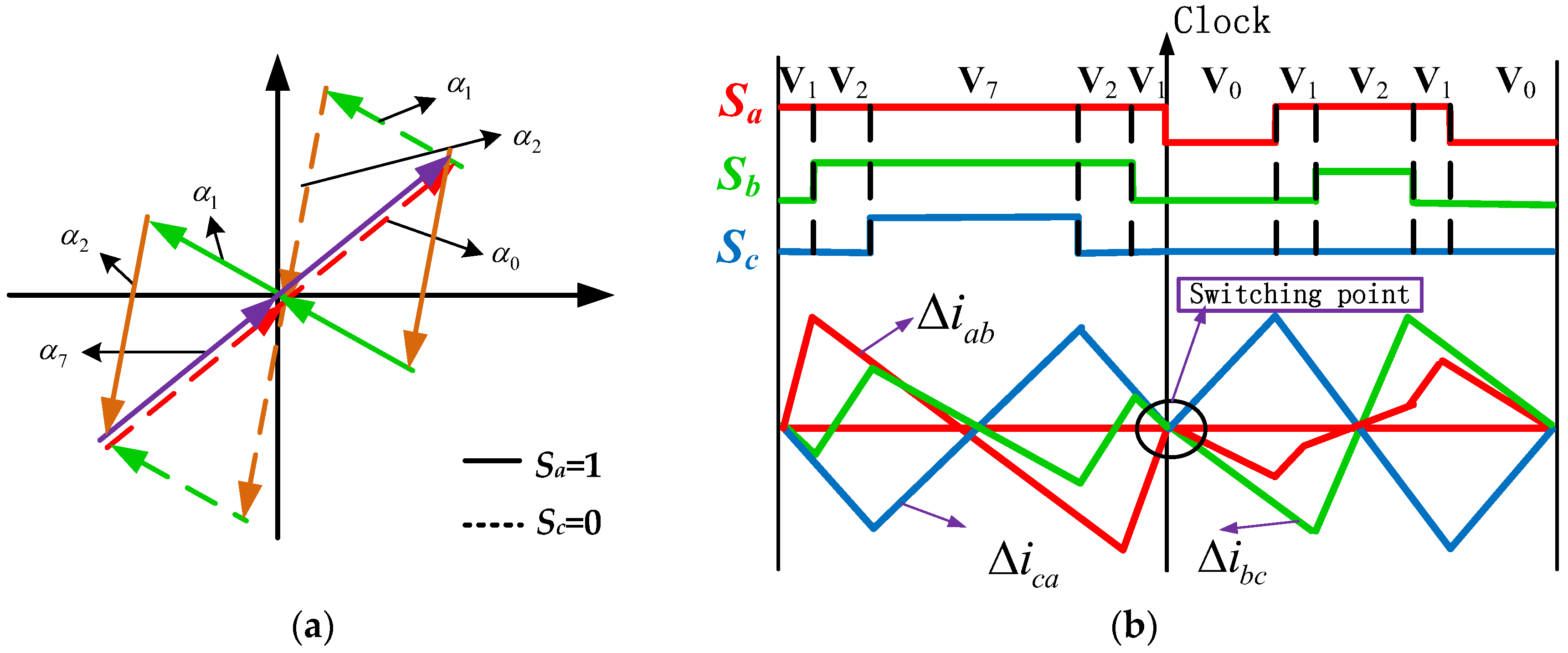
• Note that the proposed approach of variable hysteresis bandwidth is different from the conventional one, which is derived from a simplified single-phase model of a power system with APF [32,33,34]. In the ST-FHCC, the hysteresis bandwidth in the next switching period is derived from the hysteresis bandwidth in the current period according to Equation (5), which is obtained in a way that the midpoint of switch signals in the state of 0 is accurately synchronized to the clock pulse with a constant frequency, which can simultaneously realize a fixed frequency and a regulation of switch phases. In other words, two controllable current errors controlled by two switches will cross the zero point of the clock pulse accurately. As a result, the two operated switches will always operate twice during two clock pulses. Hence, the switching period will be equal to that of the clock pulse. Besides, the phases of two controllable current errors will be opposite while the two corresponding switches will be symmetrical with the switch phases regulated, as depicted in Figure 5. Since Δi_ab + Δi_bc + Δi_ca = 0, the uncontrollable current error will decrease dramatically. In addition, the operated voltage-space-vectors will all be optimal.
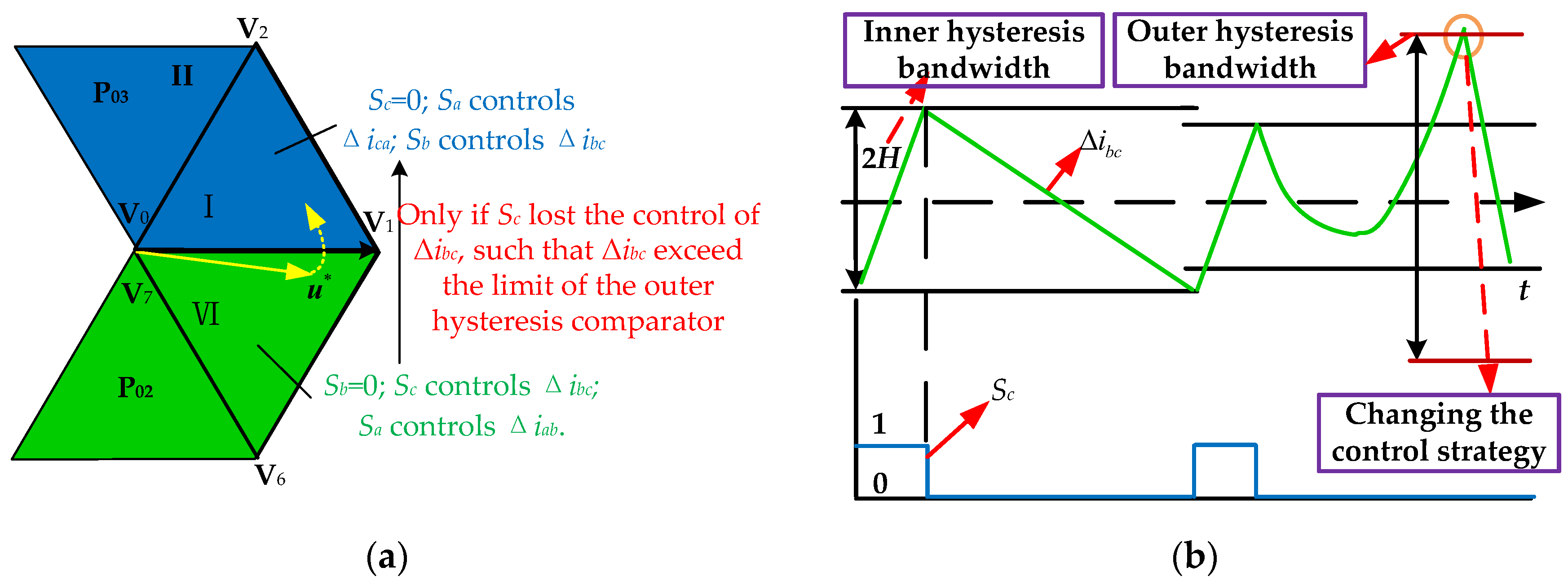
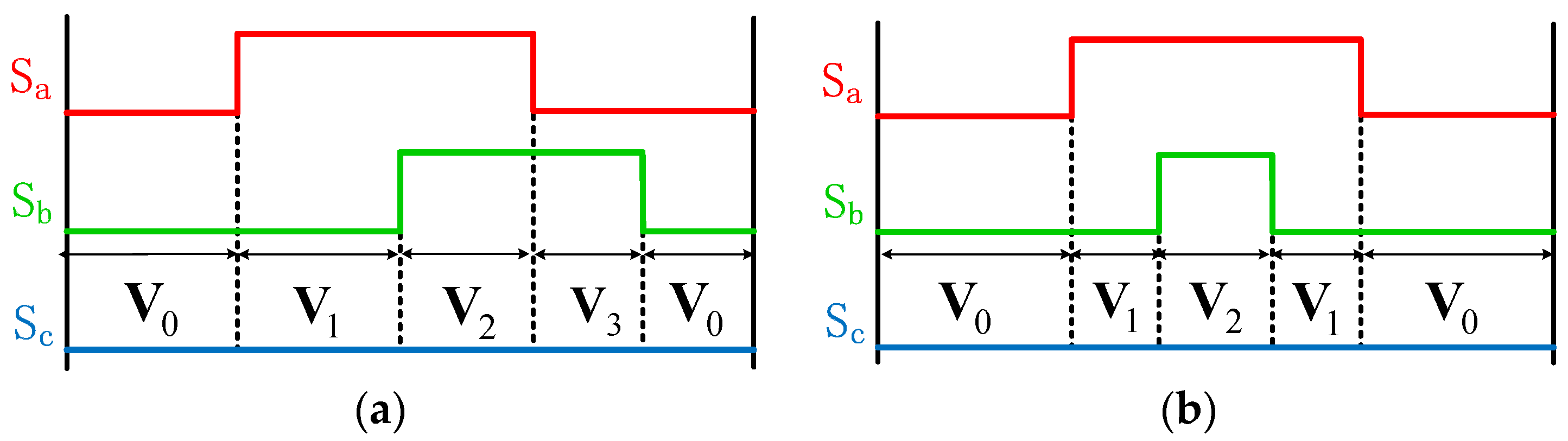
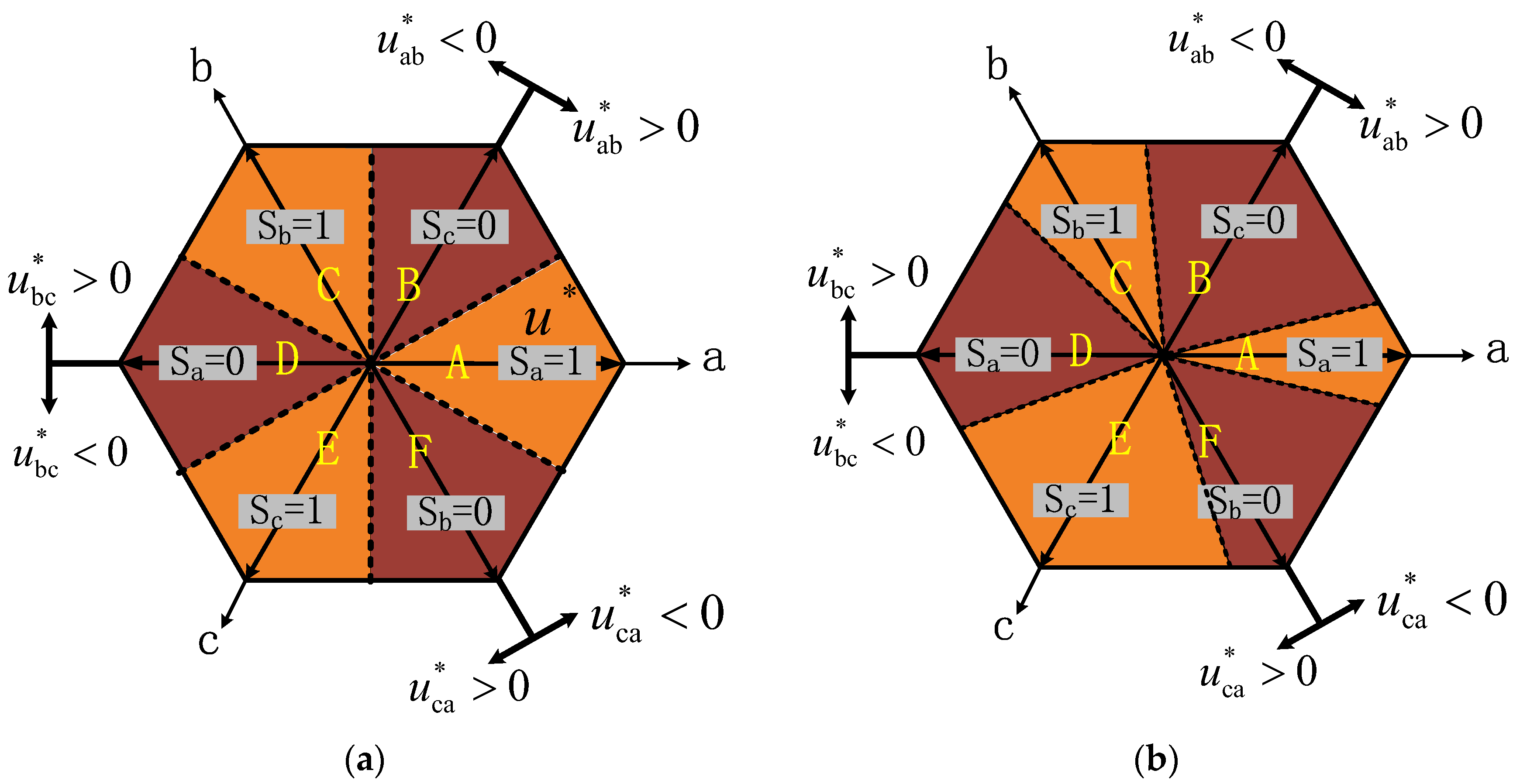
• S-FHCC is based on the division of three parallelogram regions in Figure 2, and the control strategies under mode 0 or mode 1 will be switched only if the current errors exceed the limit of the outer hysteresis bandwidth, which cannot be avoided, as illustrated in Figure 4. In contrast, ST-FHCC is based on the flexible division of six sub-regions in Figure 8, and the control strategies under mode 0 and mode 1 are switched alternatively by considering the location of u^*. The reason is that two controllable current errors are always under control by two switches no matter what control strategy under mode 0 or mode 1 is adopted in the overlapping areas produced by the parallelogram regions of mode 0 and those of mode 1. Thus, one can switch the control strategy under mode 0 (or mode 1) into that under mode 1 (or mode 0) at the zero-crossing of current errors in the overlapping areas in order to smoothly transit the boundary determined by the three parallelogram regions under mode 0 (or mode 1), as shown by Figure 7b. As a consequence, the current errors will not exceed the limit of the outer hysteresis comparator and the outer hysteresis comparator is no longer required.

7. Conclusions

In this paper, an ST-FHCC has been developed for APF. An improved approach to regulate the hysteresis bandwidth has been presented to obtain the fixed frequency and the regulation of switch phases based on OVSV. To enhance S-FHCC, a flexible division of the voltage-space-vectors diagram has been proposed and the control strategies under mode 0 and mode 1 are switched alternatively to obtain a smooth transition, which can avoid the inherent weakness of S-FHCC and improve the control accuracy of current errors. Case studies have been carried out through PSCAD/EMTDC to compare the advantages of ST-FHCC over S-FHCC. The main results and conclusions of this paper can be summarized by the following three points:

(a)

The switching frequency remains constant at 10 kHz in ST-FHCC. Moreover, the operation of voltage-space-vectors is improved via regulating the switch phases, such that the uncontrollable current error is significantly reduced and the operative voltage-space-vectors are all optimal.

(b)

A flexible division of the voltage-space-vectors diagram is proposed which divides the original diagram into six sub-regions, upon which mode 0 and mode 1 are switched alternately and smoothly. As a consequence, the inherent weakness of S-FHCC can be thoroughly overcome, e.g., the control strategies under mode 0 or mode 1 will be switched only if current errors exceed the limit of the outer hysteresis bandwidth.

(c)

Comprehensive simulation results verify that ST-FHCC can achieve a smoother, smaller, as well as more stable current error in comparison with that of S-FHCC.

A future study will apply ST-FHCC on a real APF to validate its implementation feasibility.

References

1. Yang, B.; Zhang, X.S.; Yu, T.; Shu, H.C.; Fang, Z.H. Grouped grey wolf optimizer for maximum power point tracking of doubly-fed induction generator based wind turbine. Energy Convers. Manag. 2017, 133, 427–443. [Google Scholar] [CrossRef]
2. Yang, B.; Jiang, L.; Wang, L.; Yao, W.; Wu, Q.H. Nonlinear maximum power point tracking control and modal analysis of DFIG based wind turbine. Int. J. Electr. Power Energy Syst. 2016, 74, 429–436. [Google Scholar] [CrossRef]
3. Dong, J.; Li, S.N.; Wu, S.J.; He, T.Y.; Yang, B.; Shu, H.C.; Yu, J.L. Nonlinear observer based robust passive control of DFIG for power system stability enhancement via energy reshaping. Energies 2017, 10, 1082. [Google Scholar] [CrossRef]
4. Yang, B.; Yu, T.; Shu, H.C.; Dong, J.; Jiang, L. Robust sliding-mode control of wind energy conversion systems for optimal power extraction via nonlinear perturbation observers. Appl. Energy 2018, 210, 711–723. [Google Scholar] [CrossRef]
5. Yang, B.; Yu, T.; Shu, H.C.; Zhang, X.S.; Qu, K.P.; Jiang, L. Democratic joint operations algorithm for optimal power extraction of PMSG based wind energy conversion system. Energy Convers. Manag. 2018, 159, 312–326. [Google Scholar] [CrossRef]
6. Yang, B.; Yu, T.; Shu, H.C.; Zhu, D.N.; Zeng, F.; Sang, Y.Y.; Jiang, L. Perturbation observer based fractional-order PID control of photovoltaics inverters for solar energy harvesting via Yin-Yang-Pair optimization. Energy Convers. Manag. 2018, 171, 170–187. [Google Scholar] [CrossRef]
7. Yang, B.; Yu, T.; Shu, H.C.; Zhu, D.N.; An, N.; Sang, Y.Y.; Jiang, L. Energy reshaping based passive fractional-order PID control design of a grid-connected photovoltaic inverter for optimal power extraction using grouped grey wolf optimizer. Sol. Energy 2018, 170, 31–46. [Google Scholar] [CrossRef]
8. Yang, B.; Hu, Y.L.; Huang, H.Y.; Shu, H.C.; Yu, T.; Jiang, L. Perturbation estimation based robust state feedback control for grid connected DFIG wind energy conversion system. Int. J. Hydrog. Energy 2017, 42, 20994–21005. [Google Scholar] [CrossRef]
9. Seritan, G.; Triştiu, I.; Ceaki, O.; Boboc, T. Power quality assessment for microgrid scenarios. In Proceedings of the 2016 International Conference and Exposition of Electrical and Power Engineering (EPE), Iasi, Romania, 20–22 October 2016; pp. 723–727. [Google Scholar]
10. Nieto, A.; Vita, V.; Ekonomou, L.; Mastorakis, N.E. Economic analysis of energy storage system integration with a grid connected intermittent power plant, for power quality purposes. WSEAS Trans. Power Syst. 2016, 11, 65–71. [Google Scholar]
11. Nieto, A.; Vita, V.; Maris, T.I. Power quality improvement in power grids with the integration of energy storage systems. Int. J. Eng. Res. Technol. 2016, 5, 438–443. [Google Scholar]
12. Ceaki, O.; Seritan, G.; Vatu, R.; Mancasi, M. Analysis of power quality improvement in smart grids. In Proceedings of the 10th International Symposium on Advanced Topics in Electrical Engineering (ATEE), Bucharest, Romania, 23–25 March 2017; pp. 797–801. [Google Scholar]
13. Tan, K.-H.; Lin, F.-J.; Chen, J.-H. A Three-Phase Four-Leg Inverter-Based Active Power Filter for Unbalanced Current Compensation Using a Petri Probabilistic Fuzzy Neural Network. Energies 2017, 10, 2005. [Google Scholar] [CrossRef]
14. Musa, S.; Radzi, M.A.M.; Hizam, H.; Wahab, N.I.A.; Hoon, Y.; Zainuri, M.A.A.M. Modified synchronous reference frame based shunt active power filter with fuzzy logic control pulse width modulation inverter. Energies 2017, 10, 758. [Google Scholar] [CrossRef]
15. Durna, E. Adaptive fuzzy hysteresis band current control for reducing switching losses of hybrid active power filter. IET Power Electron. 2018, 11, 937–944. [Google Scholar] [CrossRef]
16. Wu, F.; Sun, B.; Zhao, K.; Sun, L. Analysis and solution of current zero-crossing distortion with unipolar hysteresis current control in grid-connected inverter. IEEE Trans. Ind. Electron. 2013, 60, 4450–4457. [Google Scholar] [CrossRef]
17. Mao, H.; Yang, X.; Chen, Z.; Wang, Z. A hysteresis current controller for single-phase three-level voltage source inverters. IEEE Trans. Power Electron. 2012, 27, 3330–3339. [Google Scholar] [CrossRef]
18. Lam, C.S.; Wong, M.C.; Han, Y.D. Hysteresis current control of hybrid active power filters. IET Power Electron. 2012, 5, 1175–1187. [Google Scholar] [CrossRef]
19. Liu, F.; Maswood, A.I. A novel variable hysteresis band current control of three-phase three-level unity pf rectifier with constant switching frequency. IEEE Trans. Power Electron. 2006, 21, 1727–1734. [Google Scholar] [CrossRef]
20. Davoodnezhad, R.; Holmes, D.G.; McGrath, B.P. A novel three-level hysteresis current regulation strategy for three-phase three-level inverters. IEEE Trans. Power Electron. 2014, 29, 6100–6109. [Google Scholar] [CrossRef]
21. Wu, F.; Feng, F.; Luo, L.; Duan, J.; Sun, L. Sampling period online adjusting-based hysteresis current control without band with constant switching frequency. IEEE Trans. Ind. Electron. 2015, 62, 270–277. [Google Scholar] [CrossRef]
22. Ho, C.N.M.; Cheung, V.S.P.; Chung, H.S.H. Constant-frequency hysteresis current control of grid-connected VSI without bandwidth control. IEEE Trans. Power Electron. 2009, 24, 2484–2495. [Google Scholar] [CrossRef]
23. Chen, Y.; Kang, Y. The variable-bandwidth hysteresis-modulation sliding-mode control for the PWM–PFM converters. IEEE Trans. Power Electron. 2011, 26, 2727–2734. [Google Scholar] [CrossRef]
24. Suresh, Y.; Panda, A.K.; Suresh, M. Real-time implementation of adaptive fuzzy hysteresis-band current control technique for shunt active power filter. IET Power Electron. 2012, 5, 1188–1195. [Google Scholar] [CrossRef]
25. Pan, C.; Huang, Y.; Jong, T. A constant hysteresis-band current controller with fixed switching frequency. In Proceedings of the 2002 IEEE International Symposium on Industrial Electronics, L’Aquila, Italy, 8–11 July 2002; IEEE: Piscataway, NJ, USA, 2002; pp. 1021–1024. [Google Scholar]
26. Ramchand, R.; Gopakumar, K.; Patel, C.; Sivakumar, K.; Das, A.; Abu-Rub, H. Online computation of hysteresis boundary for constant switching frequency current-error space-vector-based hysteresis controller for VSI-fed IM drives. IEEE Trans. Power Electron. 2012, 27, 1521–1529. [Google Scholar] [CrossRef]
27. Holmes, D.G.; Davoodnezhad, R.; McGrath, B.P. An improved three-phase variable-band hysteresis current regulator. IEEE Trans. Power Electron. 2013, 28, 441–450. [Google Scholar] [CrossRef]
28. Kapat, S. Parameter-Insensitive Mixed-signal hysteresis-band current control for point-of-load converters with fixed frequency and robust stability. IEEE Trans. Power Electron. 2017, 32, 5760–5770. [Google Scholar] [CrossRef]
29. Fereidouni, A.; Masoum, M.A.S.; Smedley, K.M. Supervisory nearly constant frequency hysteresis current control for active power filter applications in stationary reference frame. IEEE Power Energy Technol. Syst. J. 2016, 3, 1–12. [Google Scholar] [CrossRef]
30. Zeng, J.; Yu, C.; Qi, Q. A novel hysteresis current control for active power filter with constant frequency. Electr. Power Syst. Res. 2004, 68, 75–82. [Google Scholar] [CrossRef]
31. Zeng, J.; Ni, Y.; Diao, Q.; Yuan, B.; Chen, S.; Zhang, B. Current controller for active power filter based on optimal voltage space vector. IEE Proc. Gener. Transm. Distrib. 2001, 148, 111–116. [Google Scholar] [CrossRef]
32. Vahedi, H.; Pashajavid, E.; Al-Haddad, K. Fixed-band fixed-frequency hysteresis current control used In APFs. In Proceedings of the IECON 2012—38th Annual Conference on IEEE Industrial Electronics Society, Montreal, QC, Canada, 25–28 October 2012; pp. 5944–5948. [Google Scholar]
33. Vahedi, H.; Sheikholeslami, A.; Bina, M.T. A novel hysteresis bandwidth (NHB) calculation to fix the switching frequency employed in active power filter. In Proceedings of the 2011 IEEE Applied Power Electronics Colloquium (IAPEC), Johor Bahru, Malaysia, 18–19 April 2011; pp. 155–158. [Google Scholar]
34. Vahedi, H.; Sheikholeslami, A.; Bina, M.T.; Vahedi, M. Review and simulation of fixed and adaptive hysteresis current control considering switching losses and high-frequency harmonics. Adv. Power Electron. 2011, 2011. [Google Scholar] [CrossRef]
Figure 1. Equivalent circuit of a three-phase active power filter (APF).
Energies 11 01695 g001
Figure 2. Voltage-space-vectors diagram division obtained under (a) mode 0 and (b) mode 1.
Energies 11 01695 g002
Figure 3. Switching fixed frequency hysteresis current control (S-FHCC).
Energies 11 01695 g003
Figure 4. The limit exceeding of current error resulted by the transition of u*. (a) u* moves from region VI to region I; (b) current error exceeds the limit.
Energies 11 01695 g004
Figure 5. Phase of switches is regulated.
Energies 11 01695 g005
Figure 6. Operation sequences of switches and voltage-space-vectors variation. (a) voltage-space-vectors operation without phase regulation; (b) optimal voltage space vector (OVSV) operation with phase regulation.
Energies 11 01695 g006
Figure 7. Smooth transition of voltage-space-vectors and the operation of three-phase switches. (a) u* moves from region VI to region I; (b) the operation process of the three-phase switches.
Energies 11 01695 g007
Figure 8. The flexible division of the voltage-space-vectors diagram combined with mode 0 and mode 1. (a) Symmetry division; (b) asymmetry division.
Energies 11 01695 g008
Figure 9. The ideal switching point in S-FHCC. (a) the operation sequence of voltage-space-vectors and three-phase switches; (b) the derivatives of Δi with respect to time; (c) three-phase switches operation.
Energies 11 01695 g009
Figure 10. The control mode switching in the zero-crossing point of current errors. (a) Current errors changes smoothly (S01:solid line; S11: dotted line); (b) operation of three-phase switches.
Energies 11 01695 g010
Figure 11. The overall smoothly transitive fixed frequency hysteresis current control (ST-FHCC) procedure.
Energies 11 01695 g011
Figure 12. Simulation model with APF.
Energies 11 01695 g012
Figure 13. Load current, current supplied by power system after compensation, and current error of phase a between actual current of phase a and its reference. (a) current iLa; (b) current isa; (c) current error of phase a between actual; (d) THDs of iLa and isa current of phase a and its reference.
Energies 11 01695 g013
Figure 14. The performance of the current errors obtained by S-FHCC. (a) Δiab obtained by S-FHCC; (b) detailed current errors when Δiab exceeds its limit.
Energies 11 01695 g014
Figure 15. The performance of the current errors obtained by ST-FHCC. (a) Δiab and bandwidth obtained by ST-FHCC; (b) detailed current errors at the switching point.
Energies 11 01695 g015
Figure 16. ST-FHCC performance.
Energies 11 01695 g016
Figure 17. The trajectory of the current error space-vector in the switching point. (a) S-FHCC; (b) ST-FHCC.
Energies 11 01695 g017
Figure 18. The vectorgraph of the current error. (a) S-FHCC; (b) ST-FHCC.
Energies 11 01695 g018