Forecasting the Long-Term Wind Data via Measure-Correlate-Predict (MCP) Methods

Abstract

The current study aims to forecast and analyze wind data such as wind speed at a test site called “Urumsill” on Deokjeok Island, South Korea. The measured wind data available at the aforementioned test site are only for two years (2015 and 2016), making it impossible to analyze the long-term wind characteristics. In order to overcome this problem, two measure-correlate-predict (MCP) techniques were adopted using long-term wind data (2000–2016), measured by a meteorological mast (met-mast) installed at a distance of 3 km from the test site. The wind data measured at the test site in 2016 were selected as training data to build the MCP models, whereas wind data of 2015 were used to test the accuracy of MCP models (test data). The wind data at both sites were measured at a height of 10 m and showed a good agreement for the year 2016 (training period). Using the comparison results of the year 2016, wind speed predictions were made for the rest of the years (2000–2016) at the test site. The forecasted values of wind speed had maximum relative error in the range of ±0.8 m/s for the test year of 2105. The predicted wind data values were further analyzed by estimating the mean wind speed, the Weibull shape, and the scale parameters, on a seasonal and an annual basis, in order to understand the wind behavior in the region. The accuracy and presence of possible errors in the forecasted wind data are discussed and presented.

1. Introduction

Wind energy is one of the cleanest sources for electricity production in terms of greenhouse gas (GHG) emissions. The development of new wind farms, both on-shore and off-shore, has increased rapidly over the last two decades [1]. Wind farm development is a complex process that requires a great deal of experience, analysis, and pre-feasibility studies of the selected site. Wind farm developers usually require long-term measured wind data in order to design and plan wind farms at a particular site. However, the non-availability of long-term “good quality” measured wind data hinders this process [2]. It is both impractical and nearly impossible to obtain measured long-term wind data at every planned wind farm site [3]. Many researchers have pointed out that short-term wind data sets are insufficient to predict the behavior of wind over the entire life span of a wind farm (usually 20 years) [4,5,6]. One way to address this challenge is to use computer-simulated wind data for the planned wind farm sites [5]. However, there are major issues with the availability and accuracy of such wind data. So, in this scenario, measure-correlate-predict (MCP) methods could be an alternative technique to predict long-term wind data at a planned wind farm site, where measured wind data sets are available only for a year or so [6].

In the past, it has always been a great debate to determine better techniques for wind resource forecasting. There were two popular approaches, the statistical (MCP) and the physical such as wind atlas analysis and application program (WAsP). Addison et al. [7] stated that the MCP techniques are usually more accurate and robust than the other physical modeling algorithms (WAsP [8,9]), especially in complicated terrain. Physical techniques induce uncertainties in the forecasted wind data during the prediction process. For these reasons, MCP models have been extensively applied in software applications to predict long-term wind data, and have become a standard tool for wind farm site selection. Derrick et al. [10] reported that most of the wind farm developers in 1996 used some sort of MCP method to forecast long-term wind data at test sites. The aim of the study conducted by Landberg and Mortensen [11] was to shed some light on the debate of which technique is better for predicting long-term wind data—the physical approach (e.g., WAsP) or the statistical approach (e.g., MCP). The authors stated that both techniques can predict the wind resources up to a certain degree of accuracy, but MCP is more robust, as physical methods violate flow model assumptions. Bowen and Mortensen [12] conducted a study to estimate the errors induced in the predicted wind data by WAsP due to site orography, and concluded that such errors can be significantly large. Brower [13] stated that WAsP was unable to accurately predict the long-term wind resources in hilly areas in the US due to the complex topographical nature of the test sites. However, he also mentioned that WAsP can be used in relatively flatter and less-complex terrain areas. Similarly, Prasad and Bansal [14] also stated that wind data predicted by WAsP in complex terrain can have a high amount of uncertainty. So, they concluded that it would be more feasible to utilize MCP methods while predicting wind data in complex terrains. They also concluded that uncertainty in the forecasted wind data by MCP methods could be considerably small, as the length of the time period for which measured wind data has been recorded at the test site increases. Due to the multiple advantages of MCP methods over physical methods, the current study utilized MCP algorithms.

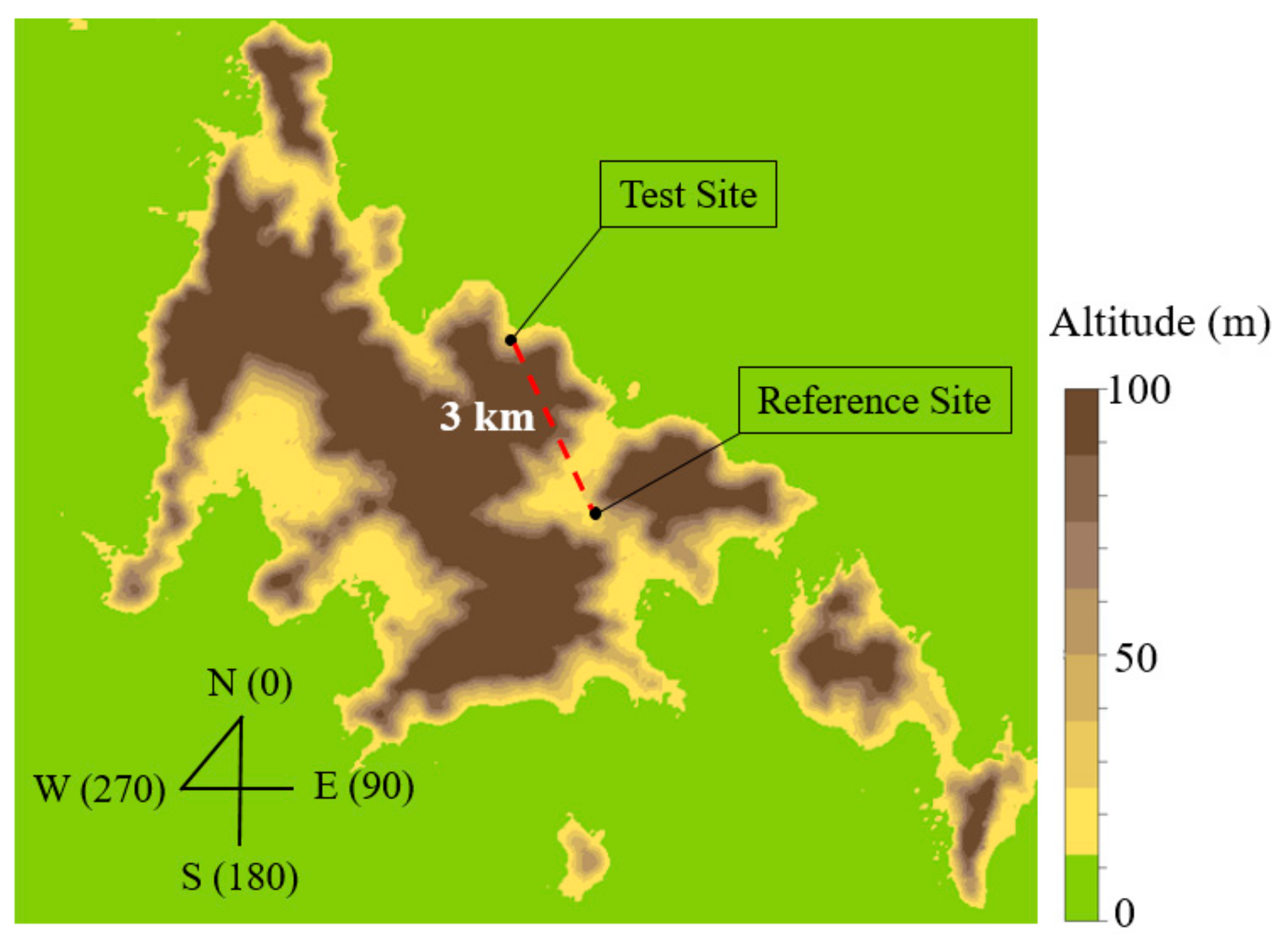
This paper investigates the forecasting of long-term wind data at a test site (Urumsill on Deokjeok Island) in South Korea, where only two years (2015 and 2016) of measured wind data is available. The Korean Meteorological Administration (KMA) has constructed and installed a meteorological mast (met-mast) near Urumsill (approximate distance is 3 km), which has been recording weather data (including wind data) continuously since 2000. The wind data recorded by the KMA was used as reference data, and the total of the seventeen years (2000–2016) of data was selected for this purpose. Recently, S. Ali et al. [15] presented a detailed statistical analysis of the wind data recorded by the KMA on Deokjeok Island.

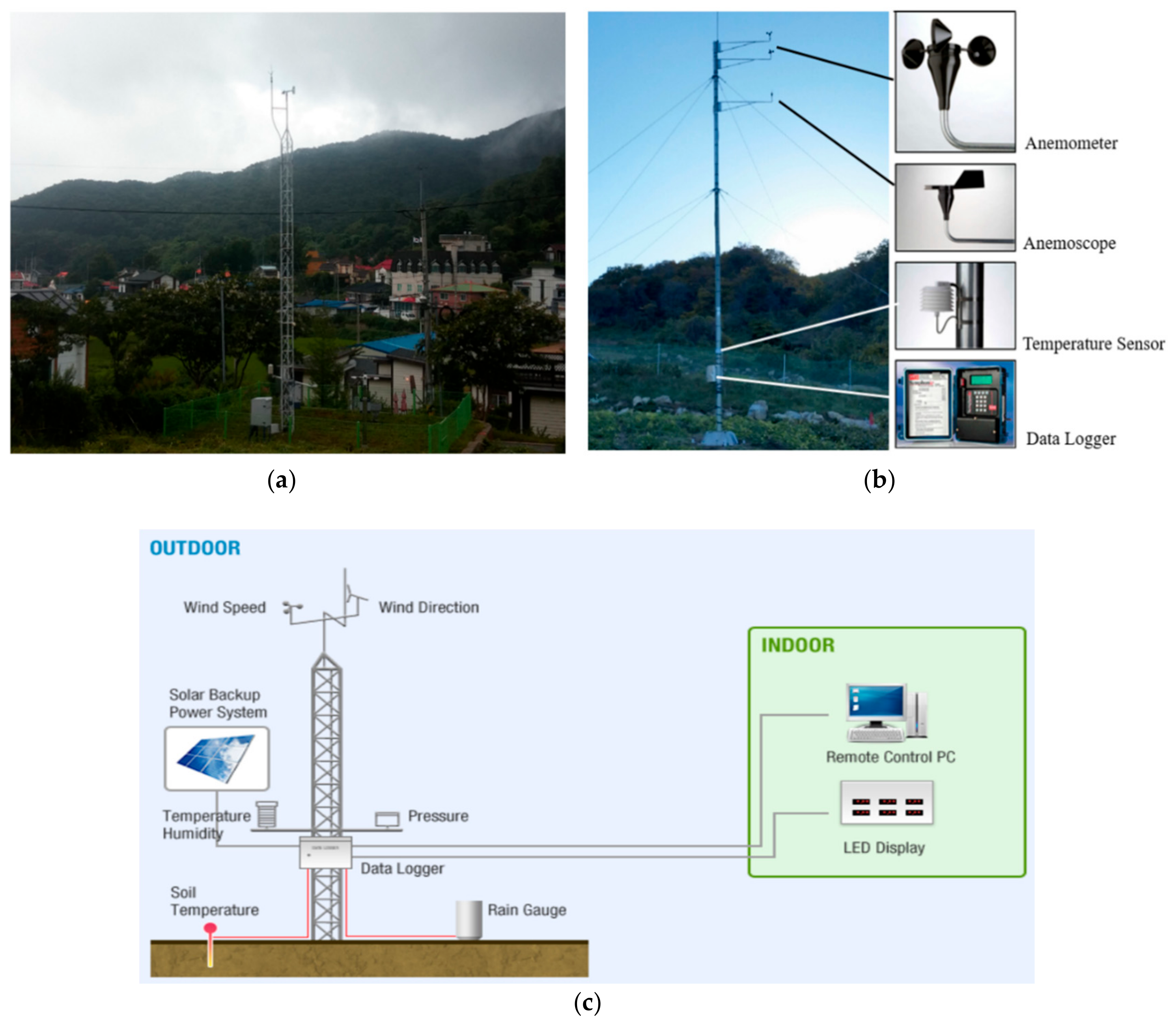
It is very important to mention that the wind data measured at the test site in year 2016 was used as training wind data to develop MCP models. Similarly, measured wind data of year 2015 was used to estimate the accuracy in the predicted values using MCP algorithms (such data are referred to as test wind data). The wind data recorded at Urumsill and the met-mast were both measured at the height of 10 m with the same time interval (10 min). So, the met-mast data could be compared against the Urumsill wind data for the training year of 2016, and in this way, long-term wind data could be determined at Urumsill via MCP methods. The height of the anemometers at both sites is also very crucial in the MCP forecasting process, as Probst and Cárdenas [16] concluded that the value of the correlation coefficient was higher between data sets when winds were measured at the same height, and vice versa for data sets collected at different heights. To the best of our knowledge, such studies had not been performed yet for this site or nearby areas. This paper not only forecasts the long-term wind data, but an estimation of wind potential will also be made at the test site. The authors believe that results presented here can be very useful for planning a wind farm development in the region.

2. Materials and Methods

2.1. Wind Data Collection at Two Sites

Prior to applying MCP methods to the data sets, it should be made sure that both sites are not too far/near to each other. Figure 1 was prepared to provide an understanding of the exact position and other geographical characteristics of the two sites. As it can be seen, the Urumsill (test site) is at least 3 km from the met-mast position (reference site) on Deokjeok Island. The height difference between both sites is approximately 60 m (test site: 80 m above sea level (ASL); reference site: 20 m ASL), and there are mountains between both sites having heights more than 100 m above sea level (ASL). The test site is situated at a higher altitude and in a more steep area as compared to the reference site. In fact, the met-mast at reference site is installed on a very flat surface, whereas the “wind master” tower at the test site is surrounded by steep mountains (see Figure 2a,b). The green color in Figure 1 represents the sea surface, whereas north is considered as the zero degree of the wind angle. This analogy will be frequently used in subsequent sections.

Table 1. (a) Wind data acquisition specifications at test site; (b) Wind data acquisition specifications at reference site [17].

(a)
Device	Parameter Recorded	Sensor Range	Accuracy (Max. Error)	Operating Temperature Range (°C)	Data Collection Period (years)	Installation Height (m)	Data Recovery Rate (%)	Original Time Interval	Averaged Time Interval	Standard Deviation (-)
NRG #40C	Wind Speed (m/s)	[1–96]	$\pm$0.1 m/s	[−55 to 60]	2015–2016	10	97	1 s	10 min	3.23
NRG #200P	Wind Angle (°)	[0–360]	$\pm$1°	[−55 to 60]	2015–2016	10	94	1 s	10 min	4.65
NRG #110S	Temperature (°C)	[−40 to 52.5]	$\pm$1.1 °C	[−40 to 52.5]	2015–2016	2	93	1 s	10 min	2.54
(b)
Device	Parameter Recorded	Sensor Range	Accuracy (Max. Error)	Operating Temperature Range (°C)	Data Collection Period (years)	Installation Height (m)	Data Recovery Rate (%)	Original Time Interval	Averaged Time Interval	Standard Deviation (-)
JY WS161C	Wind Speed (m/s)	[0–75]	$\pm$0.15 m/s	[−40 to 80]	2000–2016	10	91	1 s	10 min	4.2
JY WD160C	Wind Angle (°)	[0–360]	$\pm$3°	[−40 to 80]	2000–2016	10	98	1 s	10 min	2.9
JY100829	Temperature (°C)	[−40 to 60]	$\pm$0.1 °C	[−40 to 60]	2000–2016	2.05	97	1 s	10 min	3.1

presents the important information about the collected wind data sets at the two sites.

Originally, the wind data were recorded in one-second time intervals at both sites. However, due to the large amount of data, the original data were averaged out using a 10 min time interval and the standard deviation from the mean value of each parameter is also stated in Table 1.

Figure 2a shows the met-mast installed by the KMA in order to capture the weather data at the reference site, and Figure 2b shows a vertical tower called the “wind master”, used to record wind data at the test site. Anemometers were installed on both towers at the same height of 10 m, and the data averaging time interval was 10 min in both cases. The wind data used in the current study was recorded for seventeen years (2000–2016) by the met-mast, whereas only two years (2105 and 2016) of wind data were available at the test site.

Automatic weather systems (AWS) were designed and installed at both sites in accordance with the regulations of the WMO (World Meteorology Organization). Different sensors were attached with AWS tower to measure wind direction, wind speed, and temperature (see Table 1). All the data collected were transferred to a data logger connected with the main computer which stored the data and distributed it automatically when instructed. Figure 2c explains the overall process of wind data collection and storage in the computer.

2.2. MCP Methods

MCP algorithms compare the measured wind data sets of two sites (test and reference) over a concurrent time period (usually known as training time), in order to establish a relationship between the two data sets. Such comparisons can lead towards building a mathematical model which links wind speed at both sites in a particular fashion. Finally, these equations are utilized to predict the wind data at the test site. There are many types of MCP models (i.e., linear regression, matrix method, Weibull scale, wind index, etc.) [18]. All of these models have been extensively used by researchers globally in order to forecast long-term wind data. For instance, Ko and Huh [19] used an MCP method in order to predict the long-term wind data at a site called “Seongsan” on Jeju Island, South Korea. They discussed two MCP methods, linear and matrix, but used only the matrix method for analysis due to its robustness [20]. Sreevalsan et al. [21] adopted the linear MCP methodology in order to estimate the long-term wind data at a test site named as Majlahati. They also applied fast-Fourier transform (FFT) analysis in their study to obtain the results. The linear regression model is the more flexible and robust, and thus was deployed in the current study.

2.2.1. Method 1: The Linear Regression Model

The classical regression type of the MCP techniques was adopted in the current study in order to forecast wind speed data at a test site. Such methods compare the wind data of two sites (i.e., the test site and reference site) over a concurrent period of time. A best-fit polynomial curve of degree “n” is drawn between the two data sets. In the current case, the linear regression model was considered as it gives reasonable fits for wind energy estimations. The mathematical form of such a regression model is as follows:

$$v_{TS}=m\times v_{RS}+a,$$

(1)

where V_TS and V_RS are the wind speeds at the test site (Urumsill) and reference site (met-mast site), respectively, and, m and a are the slope and y-intercept of the best-fitting straight line. The values of the slope and the y-intercept were determined using the results of Figure 4.

2.2.2. Method 2: The Variance Ratio Model

The linear regression MCP model works on the basis of mean wind speeds. That is, it can predict the mean wind speed nearly equal to the measured mean wind speed at test site over a concurrent time period. However, if such a technique is adopted, the predicted variance is usually less than the measured variance. This creates uncertainties, biases, and errors in the predicted wind data. In order to tackle these issues, the variance ratio method was introduced [22], and it can be defined mathematically as follows:

$$v_{TS}={\overline{v}}_{TS}-\frac{({\sigma }_{TS})\left({\overline{v}}_{RS}\right)}{{\sigma }_{RS}}+\frac{({\sigma }_{TS})\left(v_{RS}\right)}{{\sigma }_{RS}},$$

(2)

where $\overline{v}$ and $\sigma$ are the mean wind speed and the standard deviation in wind speed, respectively.

2.2.3. Estimation of Errors in the Predicted Wind Data

In order to measure the variability in the estimated wind speed, two statistical parameters were introduced (i.e., the coefficient of variation, CV, and the range of variation, RV). CV determines the fluctuations in the estimated wind data around a mean value, whereas RV indicates the extremes of the wind data time series. They are calculated as follows.

$$CV(\%)=\frac{\sigma }{\overline{v}}\times 100,$$

(3)

$$RV=\frac{{\overline{v}}_{max}or{\overline{v}}_{min}-\overline{v}}{\overline{v}}.$$

(4)

In order to measure the accuracy in the predicted wind data, three statistical parameters were introduced: the ratio of mean wind speeds ($R_{\overline{v}}$), the ratio of wind speeds variance ($R_{{\sigma }^2}$), and the maximum absolute error (MAE) [22], calculated as follows:

$$R_{\overline{v}}=\frac{{{\displaystyle \sum }}_{i=1}^n{v}_{est}}{{{\displaystyle \sum }}_{i=1}^n{v}_{mes}},$$

(5)

$$R_{{\sigma }^2}=\frac{{{\displaystyle \sum }}_{i=1}^n{\left(v_{est}-{\overline{v}}_{est}\right)}^2}{{{\displaystyle \sum }}_{i=1}^n{\left(v_{mes}-{\overline{v}}_{mes}\right)}^2},$$

(6)

$$MAE=max\left|v_{est}-v_{mes}\right|,$$

(7)

where $v_{est}$ and $v_{mes}$ are the estimated and measured wind speeds, respectively. Apart from the above-mentioned error-predicting parameters, the following set of equations can also estimate the accuracy in the forecasted wind data.

$$RelativeError=ϵ=v_{est}-v_{mes},$$

(8)

$$biaserror=\overline{ϵ},$$

(9)

$$MeanSquareError=MSE=\overline{{ϵ}^2,}$$

(10)

$$RootMeanSquareError=RMSE=\sqrt{MSE},$$

(11)

$$sde=\sigma \left(ϵ\right),$$

(12)

$$sdbias=\sigma \left(v_{est}\right)-\sigma \left(v_{mes}\right).$$

(13)

The values of all of these parameters were estimated for the forecasted wind data of year 2015 and the measured test wind data of year 2015.

2.3. Estimation of Weibull Parametres

Once the wind data time series is forecasted, it can be very useful to analyze the wind data so that an estimation of wind potential can be made at the test site. Probability density functions (PDFs) are frequently used by researchers and scientists to estimate the wind potential. Over the past few years, many researchers have tried different techniques. However, from the results of previous studies it has become clear that Weibull distribution models are the most suitable for the estimation of wind potential [23,24,25]. Out of 12 probability density models, Carta et al. [26] concluded that the Weibull model has several advantages over other wind speed distribution models. Corotis et al. [27] compared the performance of Chi-squared and Weibull distributions in fitting the observed wind speed and power histograms. They came to the conclusion that both distributions can accurately predict the wind potential, but Weibull stands out for its better performance. Hennessey [28] stated that along with providing an accurate representation of wind speed distribution, Weibull can also easily estimate wind potential. Deaves and Lines [29] used a Weibull density function to fit low wind speed data, and they concluded that the Weibull model was applicable over the complete range of wind speed. The Weibull model has been applied unanimously by almost all researchers involved in wind speed data analysis. Therefore, a Weibull PDF will be used in this study to estimate the wind potential and to analyze wind characteristics. For this purpose, the Weibull probability density function (PDF) and the cumulative distribution function (CDF) were defined as follows, respectively [30].

$$WeibullPDF=f\left(v\right)=\left(\frac{k}{c}\right){\left(\frac{v}{c}\right)}^{k-1}exp\left[-{\left(\frac{v}{c}\right)}^k\right]\left(v>0;k,c>0\right),$$

(14)

$$WeibullCDF=F\left(v\right)=1-exp\left[-{\left(\frac{v}{c}\right)}^k\right].$$

(15)

$k\mathrm{and}c$ are called the Weibull shape and scale parameters, respectively. The accurate estimation of these two important parameters is of immense importance in wind energy analysis. There are numerous methods to calculate $k\mathrm{and}c$, but the current study will adopt the following five methodologies to estimate these parameters [31]:

● empirical method

$$k={\left(\frac{\sigma }{\overline{v}}\right)}^{-1.086}\left(1\le k\le 10\right),$$

(16)

$$c=\frac{\overline{v}}{\Gamma \left(1+\frac{1}{k}\right)};$$

(17)

● graphical method

$$\ln \left[-ln\left(1-F\left(v\right)\right)\right]=k\times \ln \left(v\right)-k\times \ln \left(c\right);$$

(18)

● maximum likelihood method (MLM)

$$k={\left[\frac{{{\displaystyle \sum }}_{i=1}^n{v_i}^k\ln \left(v_i\right)}{{{\displaystyle \sum }}_{i=1}^n{v_i}^k}-\frac{{{\displaystyle \sum }}_{i=1}^n\ln \left(v_i\right)}{n}\right]}^{-1},$$

(19)

$$c={\left[\frac{1}{n}{\displaystyle \sum }_{i=1}^n{v_i}^k\right]}^{1/k};$$

(20)

● power density (PD) method

$$E_{pf}=\frac{\overline{v^3}}{{\overline{v}}^3}=\frac{\Gamma (1+\frac{3}{k})}{\Gamma {(1+\frac{3}{k})}^3},$$

(21)

$$k=1+\frac{3.69}{{E_{pf}}^2},$$

(22)

where $\overline{v^3}$ is the mean of the cube of the wind speed, ${\overline{v}}^3$ is the cube of the mean wind speed, and E_pf is called the energy pattern factor, whereas c can be determined from Equation (17).

● moment method

$$\overline{v}=c\Gamma \left[1+\frac{1}{k}\right],$$

(23)

$$\sigma =c{\left[\Gamma \left(1+\frac{2}{k}\right)-{\Gamma }^2\left(1+\frac{1}{k}\right)\right]}^{1/2}.$$

(24)

In order to evaluate the performance of each of the five methods listed above, a root mean square error (RMSE) analysis was conducted. RMSE can be defined as below:

$$RMSE=\sqrt{\frac{{{\displaystyle \sum }}_{i=1}^n{\left(y_i-x_i\right)}^2}{n}},$$

(25)

where y_i is the actual value of the ith bin of wind speed, x_i is the value forecasted by the Weibull method, and n is the total number of wind speed data points in a particular wind data time series.

3. Results and Discussion

3.1. Wind Data Predictions at Test Site

Prior to applying any MCP model on the met-mast data, it is highly recommended to first compare the time series wind data of both locations over a concurrent time period. The aim of carrying out this preliminary process was to determine whether both wind data sets had similar patterns with respect to time. Figure 3 shows the season-wise results of such comparisons over a concurrent time period of five days. As can be seen in the figures, both data sets had similar patterns with respect to time, although wind data at the reference site had slightly higher magnitude. Therefore, generalizing the results of Figure 3, it can be concluded that MCP methods can be applied to the remainder of the wind data sets as well.

Figure 4 shows the wind speed data comparison for both sites measured during training year 2016. All the wind data presented in this figure are 10 min averages and measured at a height of 10 m. A straight best-fit line was passed through the data in order to obtain the slope and the y-intercept of Equation (1). The value for the square of the correlation coefficient (R²) was 86%, which is considered to be a reliable fit for the wind data. Wind speed data at the test site seemed to have a slightly higher magnitude than that of the reference site.

After obtaining the values of the slope and the y-intercept from Figure 4, the following equation of a straight line can be obtained.

$$v_{TS}=0.516\times v_{RS}+0.231.$$

(26)

Using the results of Figure 4 and Equation (26), a wind data time series was forecasted at the test site for all the considered years (2000–2016) according to method 1.

Similarly, in order to forecast wind data using method 2,

Table 2. Characteristics of the measured wind speed for the training year 2016.

Site	Mean Wind Speed (m/s)	SD in Wind Speed
Test site	2.86	1.45
Reference site	3.11	1.75

was prepared, which contains the values of the mean wind speeds and the standard deviations at both sites.

Inserting the values of Table 2 in Equation (2), the following wind data forecasting equation was obtained for method 2.

$$v_{TS}=0.828\times v_{RS}+0.283.$$

(27)

After forecasting the seventeen years (2000–2016) of wind data at the test site using both methods, it was decided to assess the accuracy of both methods. For this purpose, measured wind data of 2015 at the test site were used as test data to compare with forecasted data of the same year.

Table 3. Month-wise values of the coefficient of variation (CV) and range of variation (RV) for the test year 2015.

Test year	Method 1 (Linear Regression)			Method 2 (Variance Ratio)			Measured Wind Data (2015)
Month	CV	RVmin	RVmax	CV	RVmin	RVmax	CV	RVmin	RVmax
January	0.712	−0.940	1.618	0.565	−0.904	1.813	0.625	−1	2.005
February	0.562	−0.899	2.132	0.552	−0.892	1.778	0.619	−1	1.992
March	0.660	−0.933	2.610	0.594	−0.890	2.490	0.667	−1	2.798
April	0.482	−0.723	4.676	0.468	−0.714	2.240	0.656	−1	3.139
May	0.662	−0.736	1.787	0.402	−0.693	1.317	0.580	−1	1.899
June	0.669	−0.702	1.580	0.416	−0.676	1.489	0.615	−1	2.203
July	0.671	−0.685	2.688	0.558	−0.756	2.635	0.738	−1	3.486
August	0.483	−0.766	2.176	0.489	−0.727	2.112	0.673	−1	2.903
September	0.499	−0.765	2.133	0.403	−0.757	1.348	0.532	−1	1.780
October	0.587	−0.913	3.162	0.560	−0.924	3.896	0.606	−1	4.217
November	0.668	−0.949	2.989	0.557	−0.931	2.175	0.598	−1	2.336
December	0.678	−0.901	2.534	0.550	−0.940	1.776	0.585	−1	1.890

presents the month-wise values of CV and RV in the predicted wind data at the test site for the test year 2015. Experimental values of these variables are also presented so that a comparison can be made among the forecasted and measured data.

From the results of Table 3, it is clear that method 2 (variance ratio) was more accurate than method 1 (linear regression). Therefore, the following sections contain results which were obtained by adopting method 2 only.

3.2. Forecasted vs. Measured Wind Data at Test Site (Test Year 2015 Only)

Before analyzing the forecasted wind data, it was useful to first compare it with the measured wind data at the test site. Doing so increased the confidence in the results obtained from the analysis of the forecasted wind data. Figure 5 shows the season-wise comparison results of the predicted and the measured wind speed data at the test site. Because the measured data at the test site was available only for the years 2015 and 2016, Figure 5 was prepared using wind data of only the year 2015 (test data), for both the measured and the predicted case. As it is clear from Figure 5 that the wind data predictions showed good agreement with the measured data, the forecasted wind data could be used for further analysis. Although the predicted wind data was slightly over-estimated, the minimum r-squared (R²) value was 79%, which is acceptable.

Similarly,

Table 4. Month-wise error estimation in the predicted wind speed of test year 2015.

Month	${\mathit{v}}_{\mathit{m}\mathit{e}\mathit{s}}$ (m/s)	${\mathit{v}}_{\mathit{e}\mathit{s}\mathit{t}}$ (m/s)	${\mathit{R}}_{\overline{\mathit{v}}}$ (-)	${\mathit{R}}_{{\mathit{\sigma }}^2}$ (-)	MAE (m/s)	bias (m/s)	MSE (m2/s2)	RMSE (m/s)	sde (m/s)	sdbias (m/s)
January	2.396	2.432	1.015	0.918	0.357	0.037	0.016	0.128	0.123	−0.123
February	2.106	2.166	1.029	0.918	0.284	0.060	0.015	0.123	0.107	−0.107
March	2.054	2.118	1.031	0.918	0.407	0.065	0.017	0.130	0.112	−0.112
April	2.054	2.558	1.245	0.889	0.212	0.504	0.276	0.526	0.150	−0.150
May	1.863	2.388	1.282	0.889	0.133	0.525	0.290	0.539	0.120	−0.120
June	1.717	2.259	1.315	0.889	0.122	0.541	0.307	0.554	0.117	−0.117
July	1.605	1.905	1.187	0.897	0.277	0.300	0.105	0.324	0.122	−0.122
August	1.383	1.706	1.233	0.897	0.091	0.323	0.113	0.336	0.096	−0.096
September	1.619	1.917	1.184	0.897	0.002	0.298	0.097	0.311	0.089	−0.089
October	1.725	1.880	1.090	1.007	0.206	0.155	0.024	0.155	0.007	0.007
November	1.918	2.075	1.082	1.007	0.188	0.156	0.025	0.157	0.008	0.008
December	2.214	2.373	1.072	1.007	0.188	0.159	0.025	0.159	0.009	0.009

displays the monthly values of the mean wind speeds, estimated using the measured and forecasted wind data for the year 2015 at the test site. Along with mean wind speed, other statistical parameters ($R_{\overline{v}}$, $R_{{\sigma }^2}$, MAE, etc.) are also listed in Table 4, so that the accuracy of the forecasted wind data can be assessed.

Furthermore, Figure 6 shows the season-wise plots of relative error $\left(ϵ\right)$ estimated in the forecasted wind data for the test year 2015 on an hourly basis. It is clear from Figure 6 that the forecasted values of wind speed had maximum relative error in the range of $\pm$0.8 m/s for the test year of 2015, which can be considered as acceptable. Therefore, results of Figure 5 and Figure 6 and Table 4 suggest that wind data forecasting was completed successfully and the small amount of error can be neglected.

3.3. Analysis of Predicted Wind Data

After forecasting the wind data and measuring its accuracy, this section presents some useful analysis and results, which were prepared using the forecasted wind data. Figure 7 shows the annual variation in the Weibull shape and scale parameters, estimated by all the methods adopted in the current study. The shape parameter shows relatively smaller fluctuations as compared to the scale factor, and had an overall mean value of approximately 1.8. On the other hand, the scale parameter suddenly dropped to a value of 1 m/s from year 2009 and continued onward.

Table 5. Annual values of root mean square error (RMSE) for the forecasted wind data at the test site.

Year	Empirical	Graphical	MLM	PD	Moment
2000	0.0544	0.0945	0.0789	0.0857	0.0673
2001	0.0654	0.0912	0.0742	0.0757	0.0612
2002	0.0523	0.0892	0.0798	0.0754	0.0844
2003	0.0623	0.0932	0.0843	0.0986	0.0566
2004	0.0784	0.0746	0.0678	0.0785	0.0765
2005	0.0456	0.0845	0.0760	0.0886	0.0712
2006	0.0543	0.0759	0.0557	0.0675	0.0435
2007	0.0499	0.0893	0.0877	0.0576	0.0976
2008	0.0433	0.0783	0.0674	0.0765	0.0679
2009	0.0353	0.0865	0.0765	0.0876	0.0612
2010	0.0435	0.0678	0.0754	0.0567	0.0745
2011	0.0543	0.0674	0.0712	0.0966	0.0563
2012	0.0564	0.0874	0.0675	0.0523	0.0744
2013	0.0342	0.0923	0.0654	0.0756	0.0598
2014	0.0756	0.0765	0.0782	0.0674	0.0855
2015	0.0455	0.0876	0.0853	0.0546	0.0435
2016	0.0875	0.0956	0.0456	0.0356	0.0635
Overall	0.0552	0.0842	0.0728	0.0724	0.0673

contains the annual RMSE values estimated by all methods. In an ideal case, the RMSE value should be zero, but this is practically not possible. So, the lowest RMSE value indicates the most accurate method used to estimate the Weibull parameters. From Table 5, it is clear that the empirical method produced the overall lowest values of RMSE. Therefore, all of the following results are presented using the Weibull values estimated by the empirical method.

Figure 8 shows the season-wise plots of Weibull PDF and CDF, prepared by using all the forecasted wind data.

It can be noted that most of the wind speeds were in the range of 1–4 m/s, and 95% of the total winds were below 6 m/s, regardless of the season. Relatively lower magnitudes of wind speeds were observed during the winter and the summer as compared to other seasons. The most frequently occurring wind speeds were 2 m/s in the winter and the summer and 3 m/s in the spring and the autumn.

Similarly, Figure 9 shows the typical wind rose diagrams prepared by using all the forecasted wind data on a seasonal basis. The wind rose diagrams summarize the wind characteristics for a specific time period. It is very important to assess the prevailing wind directions to determine the layout of the wind turbines to minimize the wake loss. From the wind rose diagrams, it is clear that during all the seasons most winds came from either the north-east (NE) (45 °) or the south-west (SW) (180° to 225°), with a maximum magnitude below 4 m/s, and mostly between 1 m/s and 3 m/s.

4. Conclusions

The current study aimed to forecast and analyze the long-term wind data at a test site called “Urumsill” on Deokjeok Island, South Korea, at which only two years (2015 and 2016) of measured wind data were originally available. The reference wind data were recorded by a met-mast continuously since the year 2000, and that met-mast was located at a distance of 3 km from Urumsill. At the test site, measured wind data of 2016 were used as training data to build MCP models, whereas wind data of 2015 were used to measure the accuracy in the forecasted data (test data).

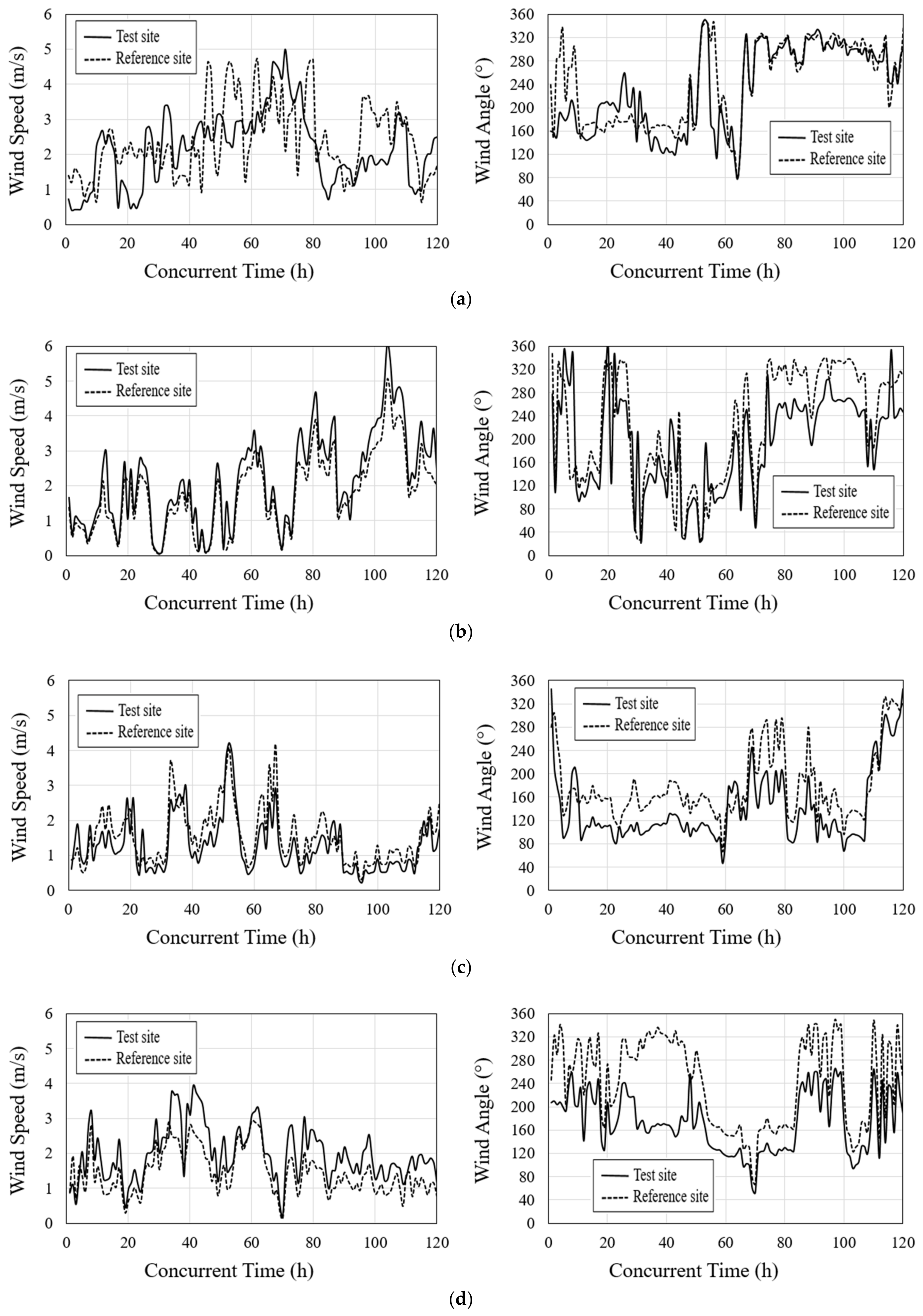
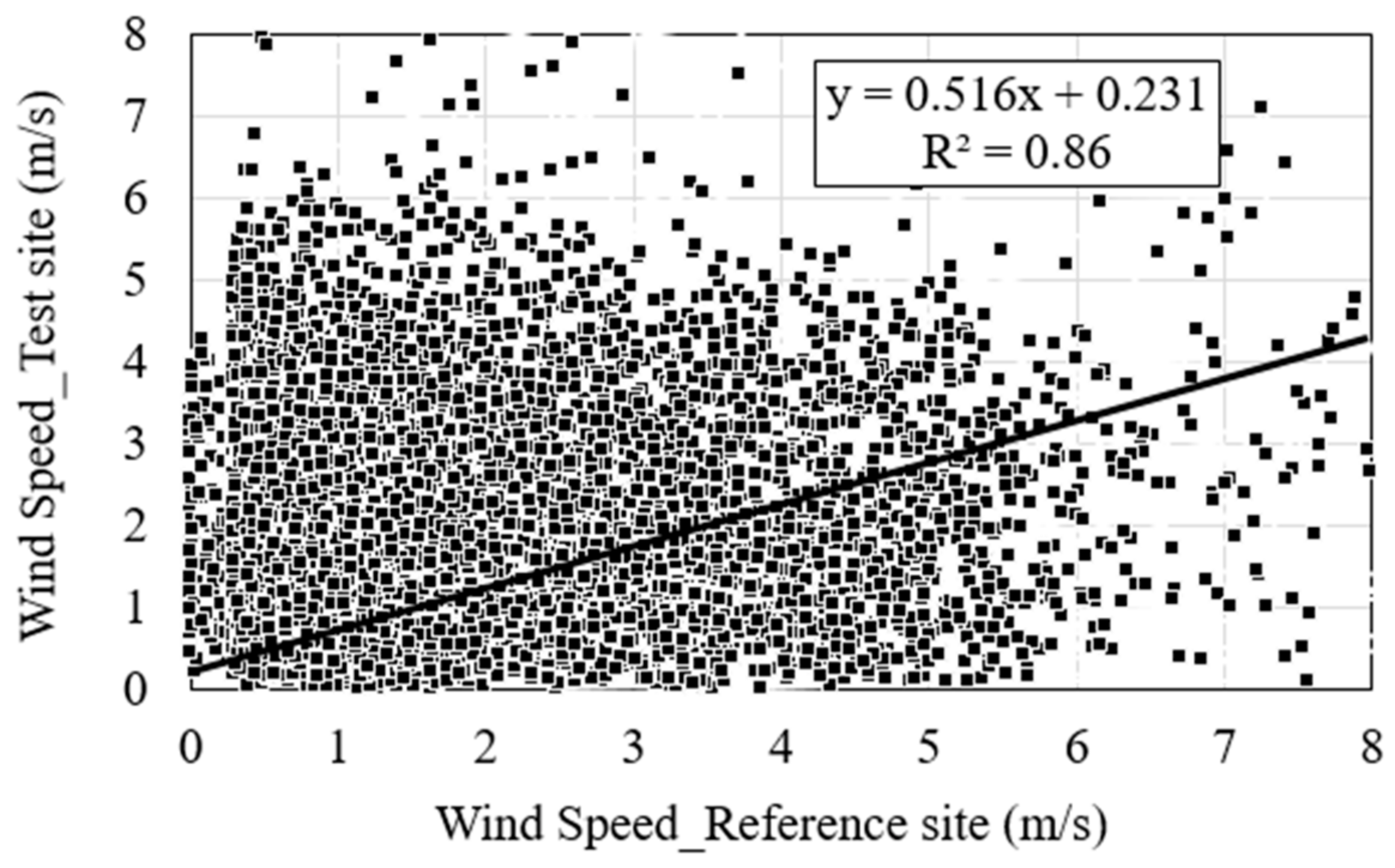
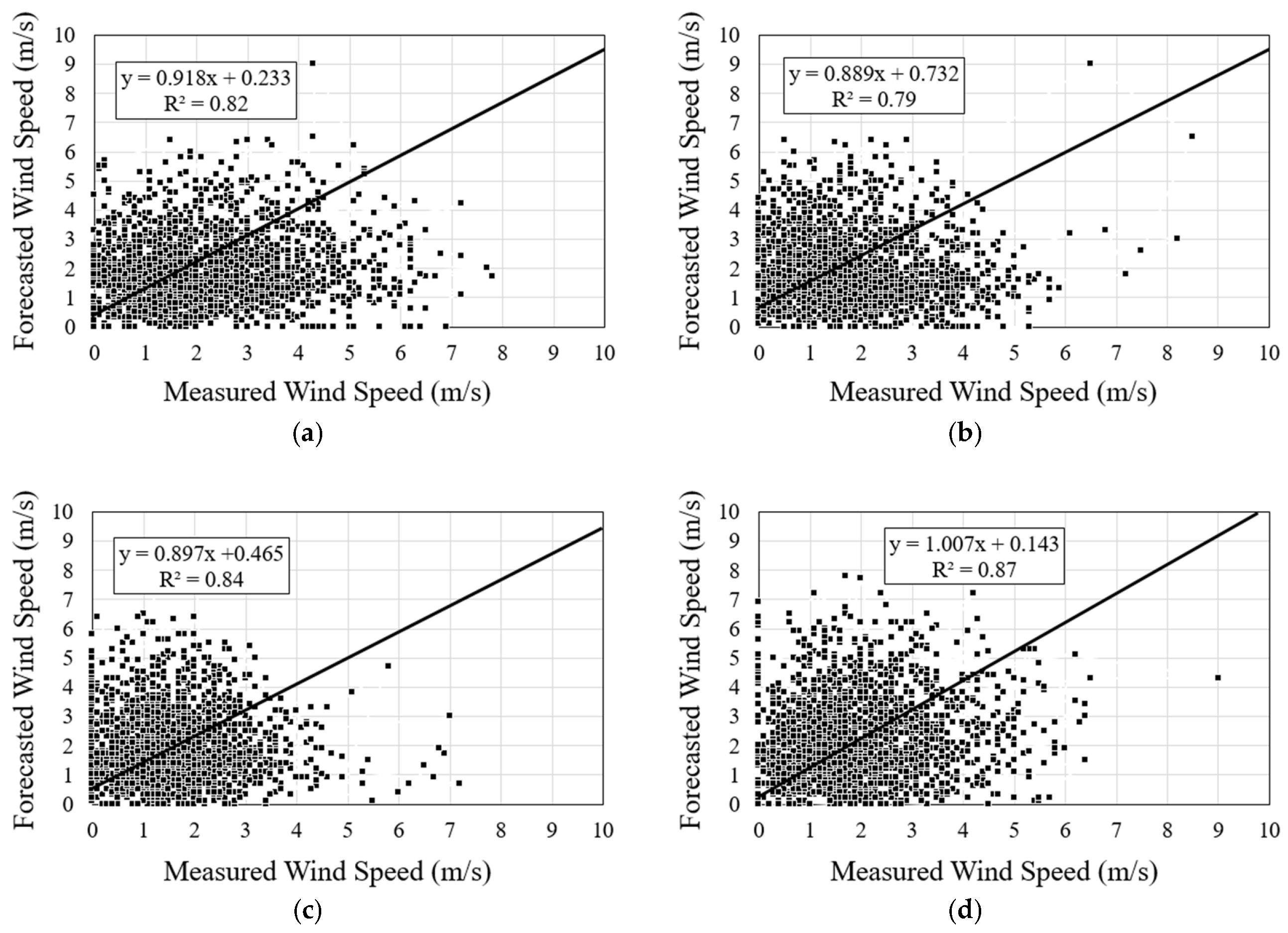
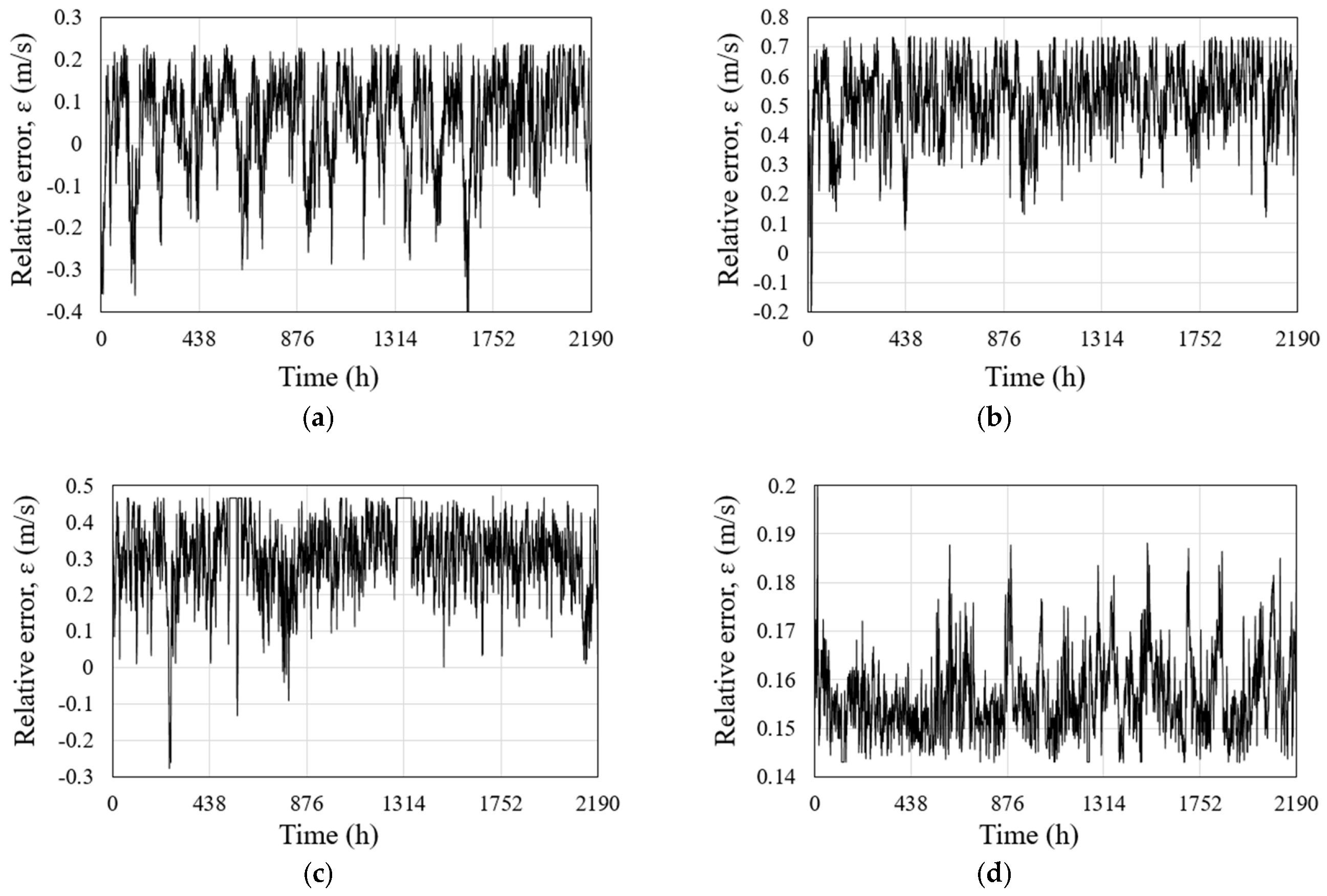
The measured wind data of both sites showed a similar pattern in wind speed and angle, over a concurrent time period of five days during all four seasons of the year 2016. When the measured wind data of both sites were compared against each other for the year 2016, the r-squared (R²) value was found to be 0.86. Similarly, on a monthly basis, the maximum value of CV was less than 0.712 and RV was found to be within [−1 to +4.676] range in the predicted wind data of the test year 2015. Measured and forecasted wind data at the test site were also compared against each other on a seasonal basis for the year 2015, and minimum R² value was found to be 0.79 (spring) in this case, which can be considered as acceptable. Furthermore, the magnitude of maximum difference between the monthly mean wind speeds of both types of data (measured vs. forecasted) corresponded to a value of 0.541 m/s, and similarly, the values of some statistical error-indicating parameters ($R_{\overline{v}}$, $R_{{\sigma }^2}$, and MAE, bias error, etc.) were also within an admissible range (over 90% accuracy). Finally, it was found that the forecasted values of wind speed had maximum relative error $\left(ϵ\right)$ in the range of $\pm$0.8 m/s for test year of 2015.

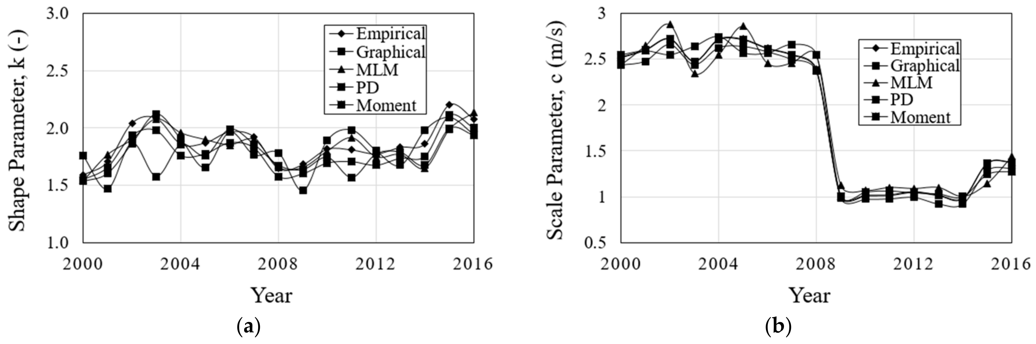
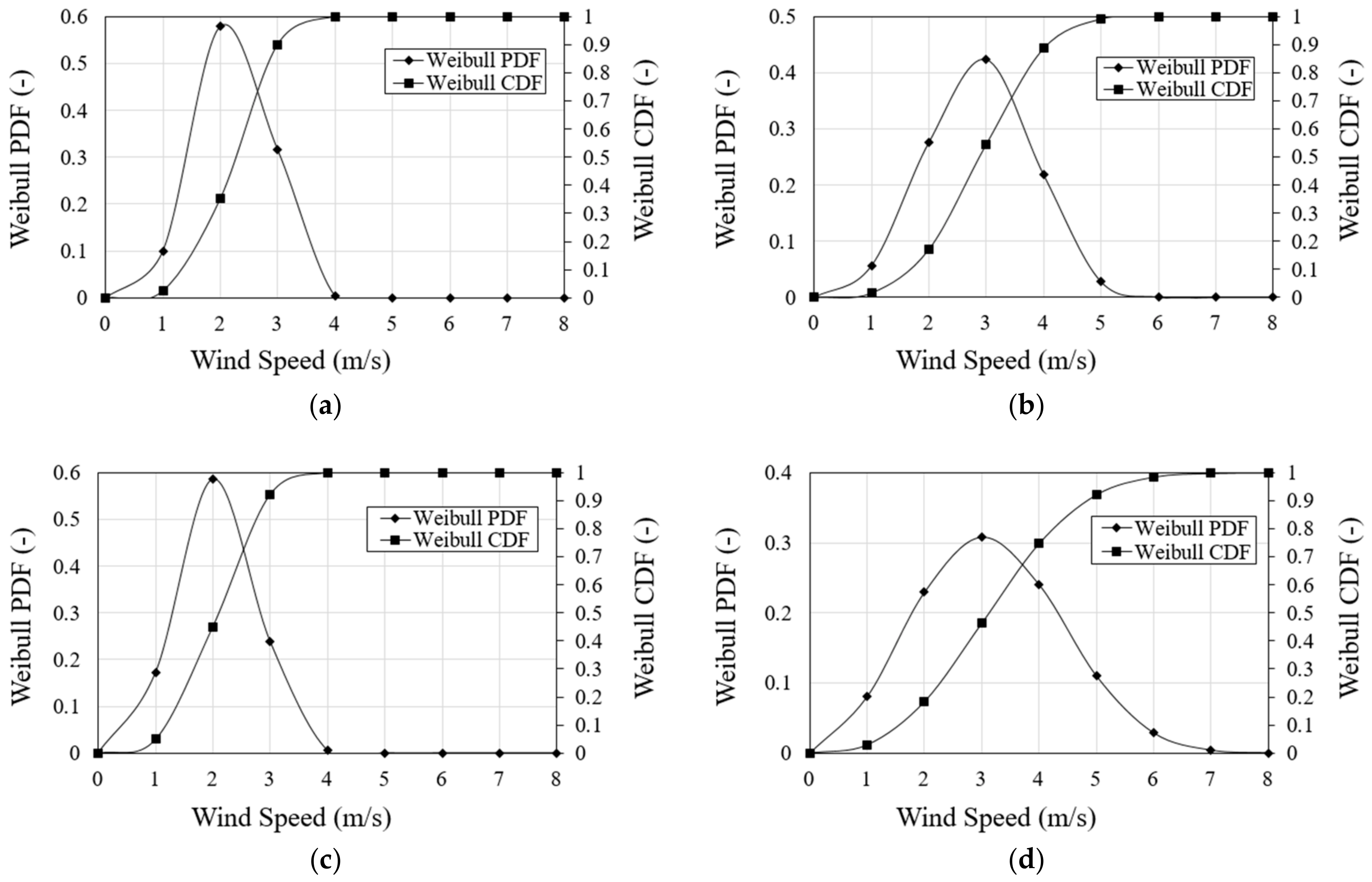
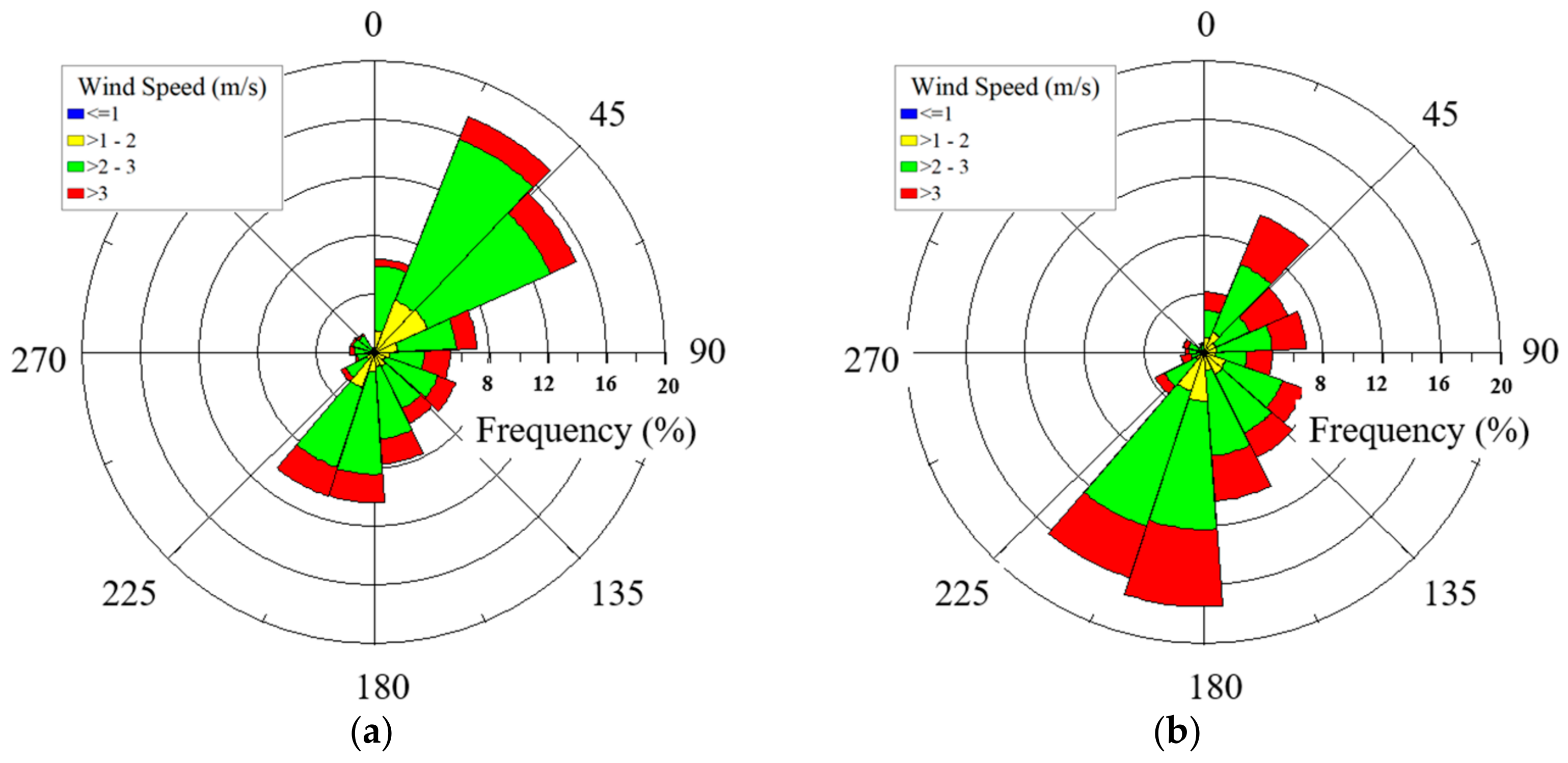
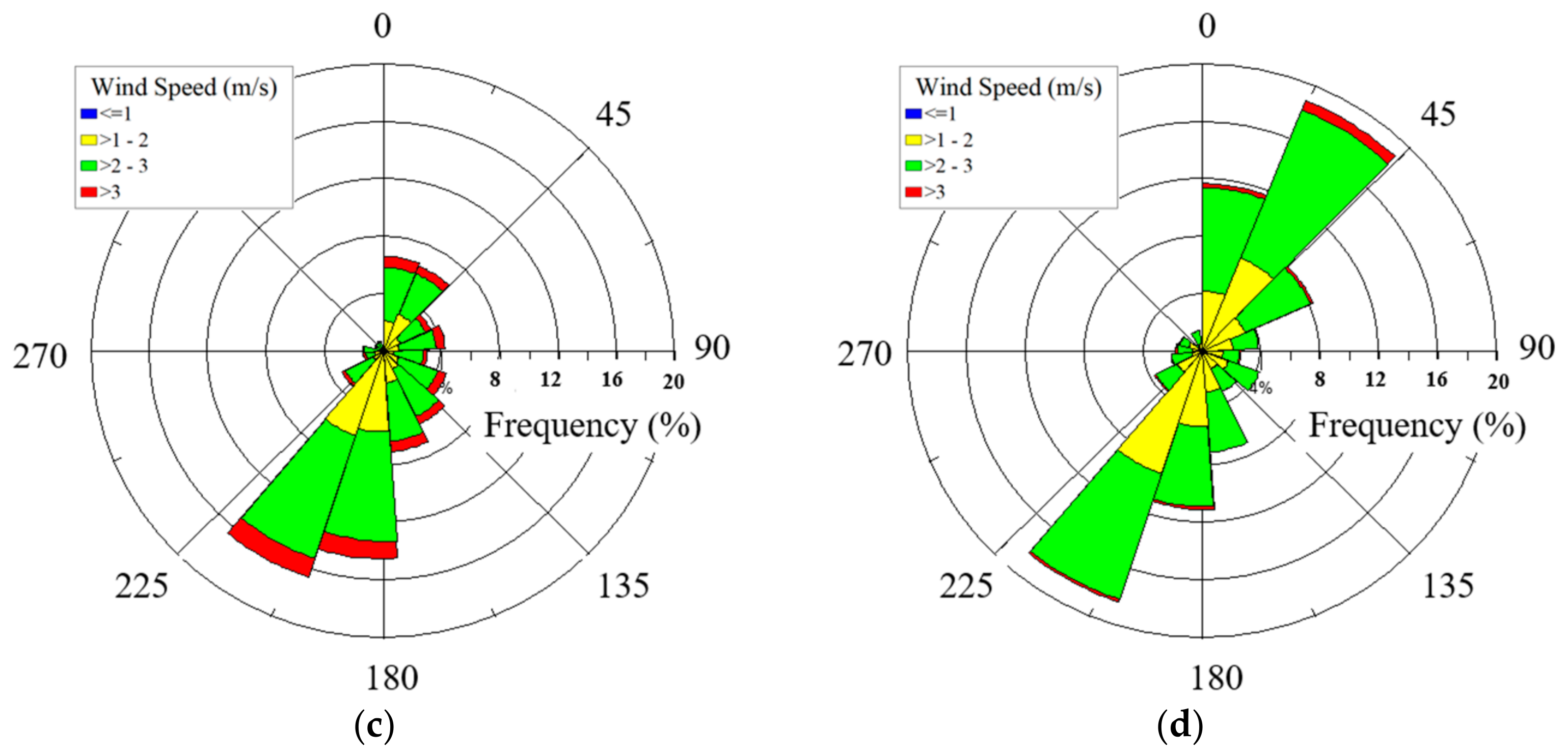
The Weibull shape (k) and scale (c) parameters were estimated for all the years (2000–2016) using five different methods according to the forecasted wind data. The empirical method was found to be the most suitable in this case, as it produced the lowest value of RMSE. Overall, the mean values of k and c were found to be 1.81 and 1.75 m/s, respectively. Most of the winds seemed to be in the range of 1 m/s to 3 m/s, and blew from either the north-east direction or the south-west direction.

References

1. Letcher, T.M. Why Wind Energy. In Wind Energy Engineering; Elsevier: New York, NY, USA, 2017; pp. 3–14. [Google Scholar]
2. Jain, P. Wind Energy Engineering; McGraw-Hill: New York, NY, USA, 2011. [Google Scholar]
3. Association, E.W.E. Wind Energy-the Facts: A Guide to the Technology, Economics and Future of Wind Power; Routledge: Abingdon, UK, 2012. [Google Scholar]
4. Hiester, T.; Pennell, W. The Siting Handbook for Large Wind Energy Systems; Wind books: Michigan, MI, USA, 1983. [Google Scholar]
5. Brower, M.; Bailey, B.H. Wind Resource Assessment; John Wiley & Sons, Inc.: Hoboken, NJ, USA, 2012. [Google Scholar]
6. Justus, C.; Mani, K.; Mikhail, A. Interannual and month-to-month variations of wind speed. J. Appl. Meteorol. 1979, 18, 913–920. [Google Scholar] [CrossRef]
7. Addison, J.D.; Hunter, A.; Bass, J.; Rebbeck, M. A neural network version of the measure correlate predict algorithm for estimating wind energy yield. In Proceedings of the 13th International Congress on Condition Monitoring and Diagnostic Engineering Management, Houston, TX, USA, 3–8 December 2000. [Google Scholar]
8. Angelis-Dimakis, A.; Biberacher, M.; Dominguez, J.; Fiorese, G.; Gadocha, S.; Gnansounou, E.; Pinedo, I. Methods and tools to evaluate the availability of renewable energy sources. Renew. Sustain. Energy Rev. 2011, 15, 1182–1200. [Google Scholar] [CrossRef] [Green Version]
9. Bowen, A.J.; Mortensen, N.G. Exploring the limits of WAsP: The wind atlas analysis and application program. In Proceedings of the 1996 European Union Wind Energy Conference, Göteborg, Sweden, 20–24 May 1996. [Google Scholar]
10. Derrick, A.; Ravey, I.; Marti, I.; Glinou, G.; Pahlke, T.; Schwenk, B.; Frandsen, S. A unified approach to the evaluation of site specific wind characteristics for use in both energy and load modelling of a potential wind turbine development site. In Proceedings of the 1997 European Wind Energy Conference, Dublin, Ireland, 6–9 October 1998. [Google Scholar]
11. Landberg, L.; Mortensen, N. A comparison of physical and statistical methods for estimating the wind resource at a site. In Proceedings of the 15th British Wind Energy Association Conference, York, UK, 5–7 October 1994. [Google Scholar]
12. Bowen, A.J.; Mortensen, N.G. WAsP Prediction Errors Due to Site Orography; Riso National Laboratory: Roskilde, Denmark, 2004; pp. 28–29. [Google Scholar]
13. Brower, M.C. Wind Resource Assessment, 1st ed.; Wiley: Hoboken, NJ, USA, 2012. [Google Scholar]
14. Prasad, R.D.; Bansal, R.C. Technologies and Methods Used in Wind Resource Assessment. In Handbook of Renewable Energy Technology; World Scientific: Singapore, 2011; pp. 69–97. [Google Scholar]
15. Ali, S.; Lee, S.-M.; Jang, C.-M. Statistical analysis of wind characteristics using WEIBULL and Rayleigh distributions in Deokjeok-do Island–Incheon, South Korea. Renew. Energy 2018, 123, 652–663. [Google Scholar] [CrossRef]
16. Probst, O.; Cárdenas, D. State of the art and trends in wind resource assessment. Energies 2010, 3, 1087–1141. [Google Scholar] [CrossRef]
17. Weather Data Release Portal. Available online: https://data.kma.go.kr/ (accessed on 23 March 2018).
18. Thøgersen, M.L.; Motta, M.; Sørensen, T.; Nielsen, P. Measure-correlate-predict methods: Case studies and software implementation. In Proceedings of the European Wind Energy Conference & Exhibition, Amsterdam, The Netherlands, 28–30 November 2007. [Google Scholar]
19. Ko, K.-N.; Huh, J.-C. Prediction of long-term wind speed and capacity factor using Measure-Correlate-Predict method. J. Korean Solar Energy Soc. 2012, 32, 37–43. [Google Scholar] [CrossRef]
20. Woods, J.; Watson, S. A new matrix method of predicting long-term wind roses with MCP. J. Wind Eng. Ind. Aerodyn. 1997, 66, 85–94. [Google Scholar] [CrossRef]
21. Sreevalsan, E.; Das, S.S.; Sasikumar, R.; Ramesh, M. Wind Farm Site Assessment Using Measure—Correlate-Predict (MCP) Analysis. Wind Eng. 2007, 31, 111–116. [Google Scholar] [CrossRef]
22. Zhang, J.; Chowdhury, S.; Messac, A.; Hodge, B.-M. Assessing long-term wind conditions by combining different measure-correlate-predict algorithms. In Proceedings of the ASME 2013 International Design Engineering Technical Conferences and Computers and Information in Engineering Conference, Portland, OR, USA, 4–7 August 2013. [Google Scholar]
23. Mohammadi, K.; Alavi, O.; Mostafaeipour, A.; Goudarzi, N.; Jalilvand, M. Assessing different parameters estimation methods of Weibull distribution to compute wind power density. Energy Convers. Manag. 2016, 108, 322–335. [Google Scholar] [CrossRef]
24. Akgül, F.G.; Şenoğlu, B.; Arslan, T. An alternative distribution to Weibull for modeling the wind speed data: Inverse Weibull distribution. Energy Convers. Manag. 2016, 114, 234–240. [Google Scholar] [CrossRef]
25. Islam, M.; Saidur, R.; Rahim, N. Assessment of wind energy potentiality at Kudat and Labuan, Malaysia using Weibull distribution function. Energy 2011, 36, 985–992. [Google Scholar] [CrossRef]
26. Carta, J.A.; Ramirez, P.; Velazquez, S. A review of wind speed probability distributions used in wind energy analysis: Case studies in the Canary Islands. Renew. Sustain. Energy Rev. 2009, 13, 933–955. [Google Scholar] [CrossRef]
27. Corotis, R.B.; Sigl, A.B.; Klein, J. Probability models of wind velocity magnitude and persistence. Solar Energy 1978, 20, 483–493. [Google Scholar] [CrossRef]
28. Hennessey, J.P., Jr. Some aspects of wind power statistics. J. Appl. Meteorol. 1977, 16, 119–128. [Google Scholar] [CrossRef]
29. Deaves, D.; Lines, I. On the fitting of low mean wind speed data to the Weibull distribution. J. Wind Eng. Ind. Aerodyn. 1997, 66, 169–178. [Google Scholar] [CrossRef]
30. Ali, S.; Lee, S.-M.; Jang, C.-M. Techno-Economic Assessment of Wind Energy Potential at Three Locations in South Korea Using Long-Term Measured Wind Data. Energies 2017, 10, 1442. [Google Scholar] [CrossRef]
31. Bilir, L.; Imir, M.; Devrim, Y.; Albostan, A. An investigation on wind energy potential and small scale wind turbine performance at İncek region–Ankara, Turkey. Energy Convers. Manag. 2015, 103, 910–923. [Google Scholar] [CrossRef]
Figure 1. Geographical locations of the two sites.
Energies 11 01541 g001
Figure 2. Wind data measuring apparatuses at both sites (a) Reference site; (b) Test site; (c) Automatic weather systems (AWS) data collection process (http://www.jinyangind.com/system_aws.html).
Energies 11 01541 g002
Figure 3. Wind data comparison at both sites over concurrent time period of five days for training year 2016. (a) Winter (1 January–5 January); (b) Spring (1 April–5 April); (c) Summer (1 July–5 July); (d) Autumn (1 October–5 October).
Energies 11 01541 g003
Figure 4. Measured wind speed comparison at both sites for training year 2016.
Energies 11 01541 g004
Figure 5. Season-wise comparison of the predicted and measured wind speed at the test site for the year 2015: (a) Winter; (b) Spring; (c) Summer; (d) Autumn.
Energies 11 01541 g005
Figure 6. Season-wise estimation of relative error in the predicted wind speed at the test site for the year 2015: (a) Winter; (b) Spring; (c) Summer; (d) Autumn.
Energies 11 01541 g006
Figure 7. Estimations of the Weibull parameters at the test site using predicted data: (a) Shape parameter; (b) Scale parameter. MLM: maximum likelihood method; PD: power density.
Energies 11 01541 g007
Figure 8. Season-wise plots of Weibull probability density function (PDF) and cumulative distribution function (CDF) at the test site using all predicted wind data: (a) Winter; (b) Spring; (c) Summer; (d) Autumn.
Energies 11 01541 g008
Figure 9. Seasonal wind rose plots at the test site using all predicted wind data: (a) Winter; (b) Spring; (c) Summer; (d) Autumn.
Energies 11 01541 g009aEnergies 11 01541 g009b