The Effect of Control Strategy on Tidal Stream Turbine Performance in Laboratory and Field Experiments

Abstract

The first aim of the research presented here is to examine the effect of turbine control by comparing a passive open-loop control strategy with a constant rotational speed proportional–integral–derivative (PID) feedback loop control applied to the same experimental turbine. The second aim is to evaluate the effect of unsteady inflow on turbine performance by comparing results from a towing-tank, in the absence of turbulence, with results from the identical machine in a tidal test site. The results will also inform the reader of: (i) the challenges of testing tidal turbines in unsteady tidal flow conditions in comparison to the controlled laboratory environment; (ii) calibration of acoustic Doppler flow measurement instruments; (iii) characterising the inflow to a turbine and identifying the uncertainties from unsteady inflow conditions by adaptation of the International Electrotechnical Commission technical specification (IEC TS): 62600-200. The research shows that maintaining a constant rotational speed with a control strategy yields a 13.7% higher peak power performance curve in the unsteady flow environment, in comparison to an open-loop control strategy. The research also shows an 8.0% higher peak power performance in the lab compared to the field, demonstrating the effect of unsteady flow conditions on power performance. The research highlights the importance of a tidal turbines control strategy when designing experiments.

1. Introduction

The economic feasibility of offshore wind energy has reached unprecedentedly low strike prices in the recent Contracts for Difference (CfD) auction in the UK at £57.50/MWh in 2022/23, dropping 43% since 2012 [1]. The offshore renewable energy sector must drive to deliver other significant technologies that can achieve competitive levelised cost of electricity (LCOE). To deliver further cost reductions in an economically sustainable manner, developers must improve their technical understanding of a technology and gain experience of its performance in the real marine environment.

Even though numerical models and various design codes and methods for rotational power generators such as wind turbines and hydropower turbines are well established and in general yield excellent results, these models still require validation through experimental testing [2,3]. It is noted from this model scale testing that Reynolds independence is a key consideration for non-dimensional comparison.

To date there is limited published research on the experimental testing of prototype devices in the marine environment. However, Gaurier et al. [4] published a study comparing the test results from the same turbine undertaken in different lab facilities. They conclude that turbulence characteristics in lab facilities need to be described more adequately to better assess performance results. Furthermore, Mycek et al. studied the effect of turbulence intensity on a model turbine in a circulating flume. The range of turbulence intensities used (3% and 15%) may be typical of what is found at a tidal test site and the results show that this change in intensity has a near negligible effect on the time averaged performance of the turbine [5].

To support the industry in understanding the challenges of tidal turbine performance assessment a series of studies have been undertaken by Queen’s University Belfast at a significant scale in tank, lake and tidal environments. The experimental campaigns are described in

Table 1. Tidal Turbine Testing (TTT) project history.

Project	Date	Experiment Description	Publications
TTT	2013–2014	◦ Tandem pushing tests in Montgomery Lake ◦ Moored tandem tests in Strangford Narrows	[6,7,8]
TTT 2	2014–2015	◦ MaRINET (Marine Renewables Infrastructure Network) transnational access to Consiglio Nazionale delle Ricerche-Istituto nazionale per studi ed esperienze di architettura navale (CNR-INSEAN) for turbine tests ◦ MaRINET transnational access to Strangford Narrows for SCHOTTEL Hydro STG 50 turbine (SCHOTTEL, Spay, Germany) tests	[9,10,11,12]
TTT 3	2015–2017	◦ Moored single turbine testing in Strangford Narrows ◦ Towing tank testing in CNR-INSEAN with Wave and Yaw Angles	[13]

and related publications are cited.

From this previous research and literature review it has been reported that experimental testing in an unsteady marine environment results in power performance disparities when compared with steady flow testing. Jeffcoate et al. [7] reports a 24% reduction in C_P between steady and unsteady flows. Meanwhile, Starzmann et al. [11] report comparable power performance between steady and unsteady flows (only a 5% change in C_P); however, the thrust performance was higher in the unsteady conditions relative to the steady conditions. In addition to this previous work, applicable studies have been conducted by other groups at a similar scale. The work of Forbush et al. [14] reports an 8% increase in performance with turbulent flow; however, the cross-flow tidal turbine used in this research sets it apart as a unique result, which may be specific to the rotor type. Blackmore et al. [15] performed repeat experiments in a circulating flume, the inflow characteristics were varied using a grid. The inflow velocity was maintained, while the Turbulence Intensity (TI) and length scale varied. The findings showed a 10% reduction in C_P with an increase in TI, conversely an increase in length scale resulted in an increase in C_P.

In all field experiment cases, the cause of power disparity between lab and field is partly attributed to uncertainty in the experiments. Further consideration of the source of uncertainty has identified two critical contributing factors:

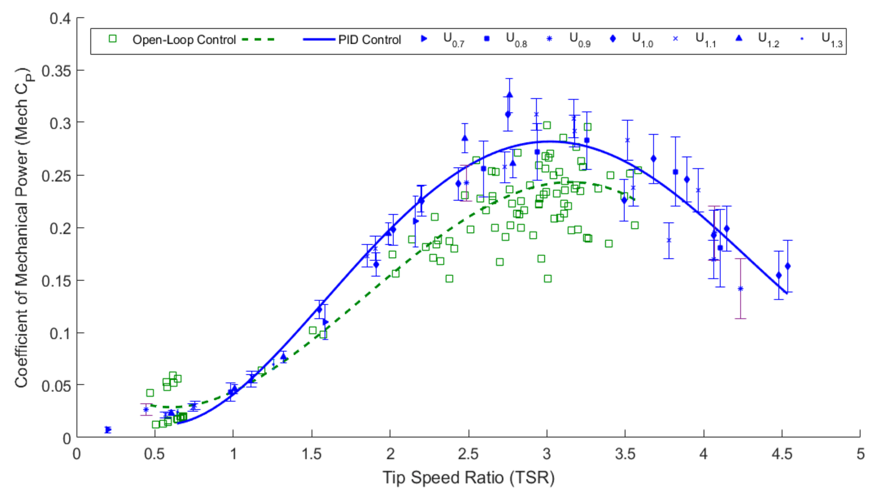
• A crucial factor in the accuracy of performance measurements arises from the control strategy imposed on the tidal turbine. The capability of the control system to keep the rotor operating near its optimum Tip Speed Ratio (TSR), when driven by an unsteady and non-uniform inflow velocity, and avoiding ‘stall’, is a key element in a successful commercial turbine. Similarly, the control strategy adopted during an experiment can increase the error bounds in derived performance indicators, such as C_P. Control strategies used in previous tidal turbine performance testing vary. For devices at low Technology Readiness Level (TRL) scales [16], such as those used in laboratory scale experiments, an open-loop control may suffice [9]. However, more commonly, a closed-loop, proportional–integral–derivative (PID) feedback control strategy is found [17,18] in higher TRL devices.
  It is recognised that in order to develop the industry, advanced control strategies require development and testing in highly parameterised conditions. Efforts are being made in this field in both research and industry. The use of overspeed, pitch or stall control strategies with peak power tracking, or surface mapping algorithms for condition monitoring purposes are under development [19,20]. Furthermore, future options may include the possibility of feed-forward algorithms such as those being trialled in the wind sector [21].
• The second source of increased uncertainty comes from the increased variability of the inflow velocity. This is of particularly significance since the power density scales with the cube of the inflow velocity. Furthermore, both genuine variability and sampling errors are compounded in real velocimetry data. Separating and quantifying their effects requires care in calibration of instruments and data analysis. In order to promote consistent best practice in the power performance testing of Tidal Energy Converters (TECs), Johnstone et al. published best practices for the wave and tidal sector [22] which specifies the requirements for clear uncertainty analysis. Further to this the IEC (Geneva, Switzerland) published a Technical Specification IEC/TS 62600-200 [23]. The specification provides the methodology for determining an average value for velocity at a site, enabling the time average performance of a turbine to be captured and reported to a common standard. The IEC specification has been used in other research projects and across the industry [10,13,24] and will be used to guide the data analysis in this paper.

In summary, the literature review has highlighted experiments where turbine testing in the lab has been compared to the field. The control strategy and inflow measurements are significant parameters that must reflect the device TRL and testing environment. In order to inform the sector of the significance of these parameters, the TTT turbine will be deployed in the lab and field, the derived performance results will be compared for two control strategies, and in a steady and unsteady inflow environment. The lab experiments will be used as an opportunity to calibrate and derive uncertainty metrics for the inflow, this will then be applied to the field experiments and performances compared.

2. Experimental Setup

Under the TTT 3 project, both the laboratory and field tests were conducted using the same instrument, maintaining continuity between experiments. This was achieved by using the same turbine, velocity instruments and data acquisition system. The laboratory experiments were undertaken in the controlled steady environment of the towing tank facility CNR-INSEAN, Italy. The field test experiments were performed in the uncontrolled, unsteady environment of the tidal test site in Strangford Narrows, Northern Ireland (Lat.: 54.381801°, Long.: −5.556743°).

The 1.5 m diameter turbine is pictured during operations in Strangford Lough in 2016 (Figure 1); the device dimensions can be found in the supplementary appendix of previous work [6] and remain consistent in this work. The rotor blades are an Eppler E387 airfoil geometry, each blade is 0.575 m long and features a pitch distribution similar to industrial wind turbine blades, with a root pitch angle of 32° which recedes to 13° at the tip of the blade. As this is not a commercial blade and is not designed to be scaled the significance of Reynolds independency is limited.

2.1. Flow Instrumentation

Acoustic Doppler profilers (ADPs) are often used for tidal flow resource assessment, and are the given method for characterising inflow conditions by the IEC [23]. The Nortek 2 MHz ‘Aquadopp’ used in the experiments was the primary instrument for determining inflow velocity in these experiments.

The experimental setup shown in this section relates to all work as part of the TTT 3 project. Please refer to referenced papers for further details on previous experimental setups [6,9]. The supporting gantry also hosts a Nortek ‘Vector’ Acoustic Doppler Velocimetry (ADV) with the sample volume located at the apex of swept area at 16 Hz, this provided insight into the inflow turbulence. The deployment parameters for both instruments are given below. In accordance with the IEC standards for power performance assessment, the inflow measurements were taken at an upstream distance of between 2–5 equivalent diameters from the plane of rotation [23].

The geometrical setup can be seen in Figure 2 and is detailed in

Table 2. Turbine, Acoustic Doppler profiler (ADP) and Acoustic Doppler Velocimetry (ADV) deployment parameters.

Parameter	ADP		ADV
	Strangford	CNR-INSEAN	Strangford	CNR-INSEAN
Distance D1 (m)	0.30 m	0.30 m	0.86 m	0.86 m
Distance D2 (m)	2.99 m	3.80 m	3.10 m	3.7 m
Distance D3 (m)	1.75 m	1.75 m	1.75 m	1.75 m
Power	high	high	high	high
Transmit length	N/A	N/A	8 mm	8 mm
Number of cells	20	20	N/A	N/A
Cell Size (m)	0.25 m	0.25 m	N/A	N/A
Blanking Distance (m)	0.25 m	0.25 m	N/A	N/A
Co-ordinate System	Beam	Beam	Beam	Beam
Sample Frequency (Hz)	1 Hz	1 Hz	16 Hz	16 Hz
Sample Period (s)	120–600 s	90–140 s	120–600 s	90–140 s

, where the parameter D2 has two values: one for the towing tank and one for Strangford Lough tests, respectively. This difference was due to the location of suitable mounting points in the towing carriage.

2.2. Flow Instrumentation Validation

Many ADP instruments have previously been independently calibrated and validated to verify the quality of factory settings. Shih et al. [25] demonstrated the close agreement between calibrations for two different ADP suppliers, RDI (Poway, CA, USA) & SonTek (San Diego, CA, USA) in a towing tank facility in 2000. More recently, Oberg et al. [26] performed similar experiments with the most recent instrument firmware, again using RDI and SonTek instruments. Little work has been found which independently calibrates the Nortek Aquadopp ADP used in this experiment; however, Elsäβer et al. showed discrepancies in time averaged velocities of up to 0.19 ms⁻¹ between two instruments collocated in the field [27]. In order to ensure instrument accuracy, the ADP (2 MHz Aquadopp) was calibrated during the towing tests under conditions as close as were possible to the field. Seeding of the towing tank was required to improve the Signal to Noise Ratio (SNR).

To validate this ADP calibration against another independent instrument while working in the field, the Nortek Vector ADV was likewise calibrated during the tank work. 16 Hz Vector data was averaged over 1-s bins to match the ADP (2 MHz Aquadopp) data bins. All the calibration results are given in

Table 3. Deviation of Nortek instruments from factory calibration.

Nortek Transform Matrix Output	ADP—Aquadopp	ADV—Vector
x	U = −1.0124x + 4.97	U = −1.0042x + 6.4
y	V = −1.0124y + 0	V = +1.0042y + 0
z	W = −1.0124z + 0	W = −1.0042z + 0
Bias in U (1 σ)	−0.03%	+0.05%
Precision in U (1 σ)	±0.6%	±0.9%

and show the deviation of the instruments from their factory calibration. Each calibration equations were derived for U, V and W from the towing tests for the Aquadopp (ADP) and Vector (ADV) instruments. The linear equations demonstrate the precision and bias drift since the previous calibration (in mm/s) as yielded by the Nortek transform matrices for each instrument. Note the signs are chosen to make the output components have the same axis convention for both instruments. U is the main direction of inflow, along the turbine axis.

In summary, the calibration performed in the towing tank agrees closely with the factory calibration, showing less than a percentage difference in bias and precision. The same individual instruments, deployment parameters and locations were used during both the laboratory and fieldwork testing. Further validation of the results has been undertaken using the fieldwork data, further detail can be found in Appendix A. This provides confidence in instrument accuracy and draws attention to the high spatial variability in tidal flows, as discussed by Elsäβer et al. [27].

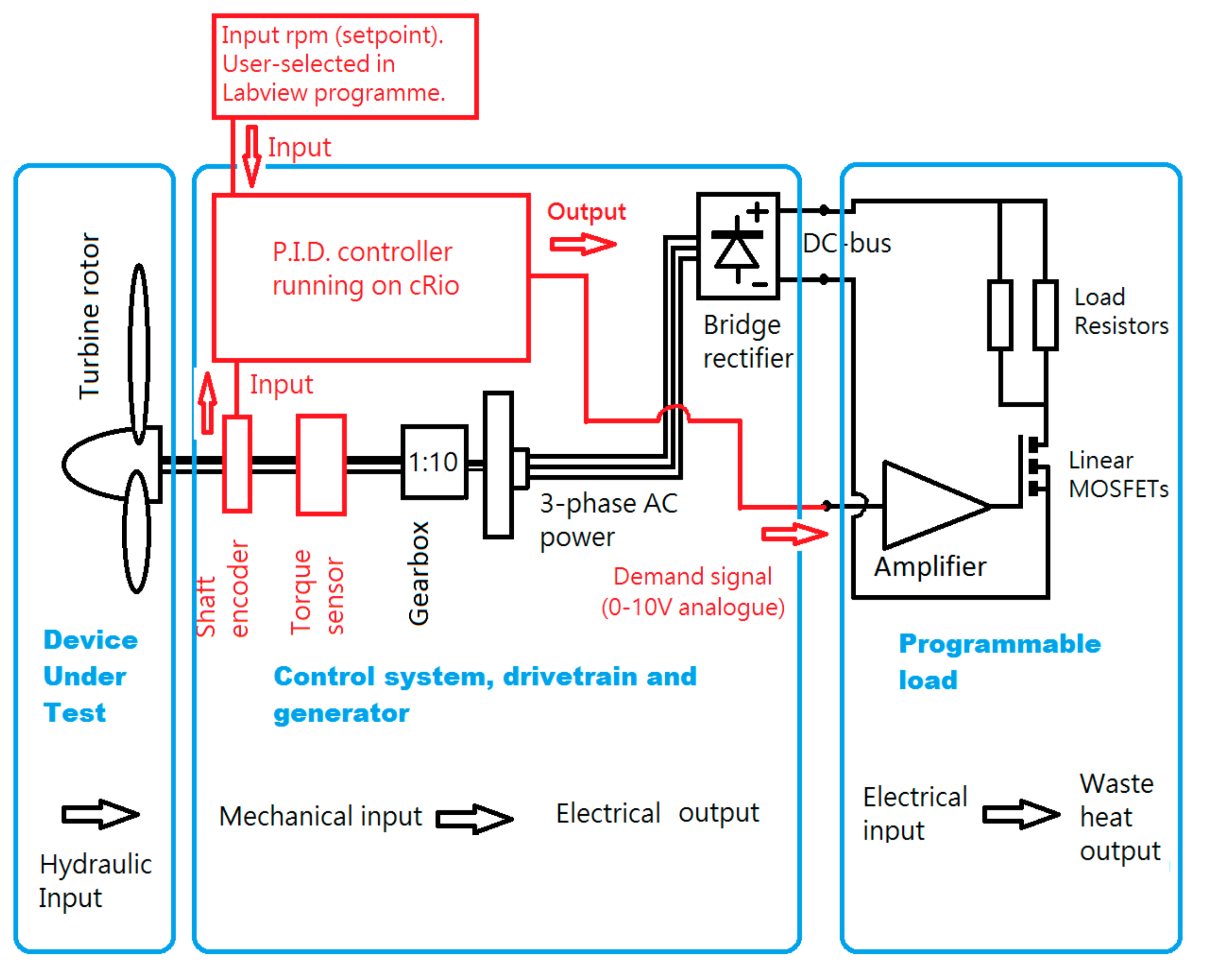
2.3. Control Strategy

The control of wind turbines is an established and mature area of technology. The control strategy involves multiple inputs and outputs [28] and more than one control loop, often extending to variables intended to optimise the performance of an array and its grid interface.

In contrast, the original TTT 2 experimental design was an open-loop load control, as shown in Figure 3. Control was provided by a binary array of resistors (5 values, each the double of the previous: 10.25 ohms, 20.5 ohms etc.). Thus, 32 load values could be placed on the DC-bus by switching combinations in and out. Electromechanical contactors select the load on command from the central Data Acquisition System (DAQ), based on a National Instruments Compact Rio (cRio) running Labview and further custom-made interface electronics and cabling.

In developing the control system, a single control loop was included with only one process variable as the input (the rotor shaft speed) and one output (the electrical demand placed on the alternator). A review of Proportional–Integral–Derivative (PID) control theory, developed in the mid 20th century, is presented by Bennet [29]. In order to incorporate a closed-loop PID load control, a linear regulator was used to place an electronic load on the turbine at the DC output terminals. The upgraded PID control loop is shown in Figure 4. An absolute rotary encoder was included to provide higher resolution of shaft speed for the PID loop.

The PID control system was run as a Labview virtual instrument in the DAQ programme, which was written specifically for the project. Most of the programme’s other features were identical for both TTT 2 (open-loop) and TTT 3 (PID; see Table 1 for project details). To control the turbine for the TTT 3 system, the user selects a chosen shaft speed (set point) and the system then attempts to maintain that speed independently of flow features in the field, or of towing speed in the laboratory. The PID parameters used were identical in both the field and towing tank; all the results under PID control were collected with the parameters set as in

Table 4. Proportional-Integral-Differential parameters.

Symbol	Description	Value
Kc	Proportional constant	2.2 (no dimensions)
Ti	Integration time constant	0.003 (min)
Td	Differential time constant	0.001 (min)

.

The proportional constant, Kc or gain was either positive or negative, depending on the rotational direction of the driveshaft. This also applied to the set RPM (Rotations per Minute) value in the control system. The tuning of the loop parameters was done in the field with the Zeigler and Nichols ‘ultimate cycling’ method [30], followed by some minor optimisation by trial and error. It is worth noting that the ultimate cycling method gave adequate robustness and precision of control for our purposes and was only slightly adjusted with subsequent trial and error.

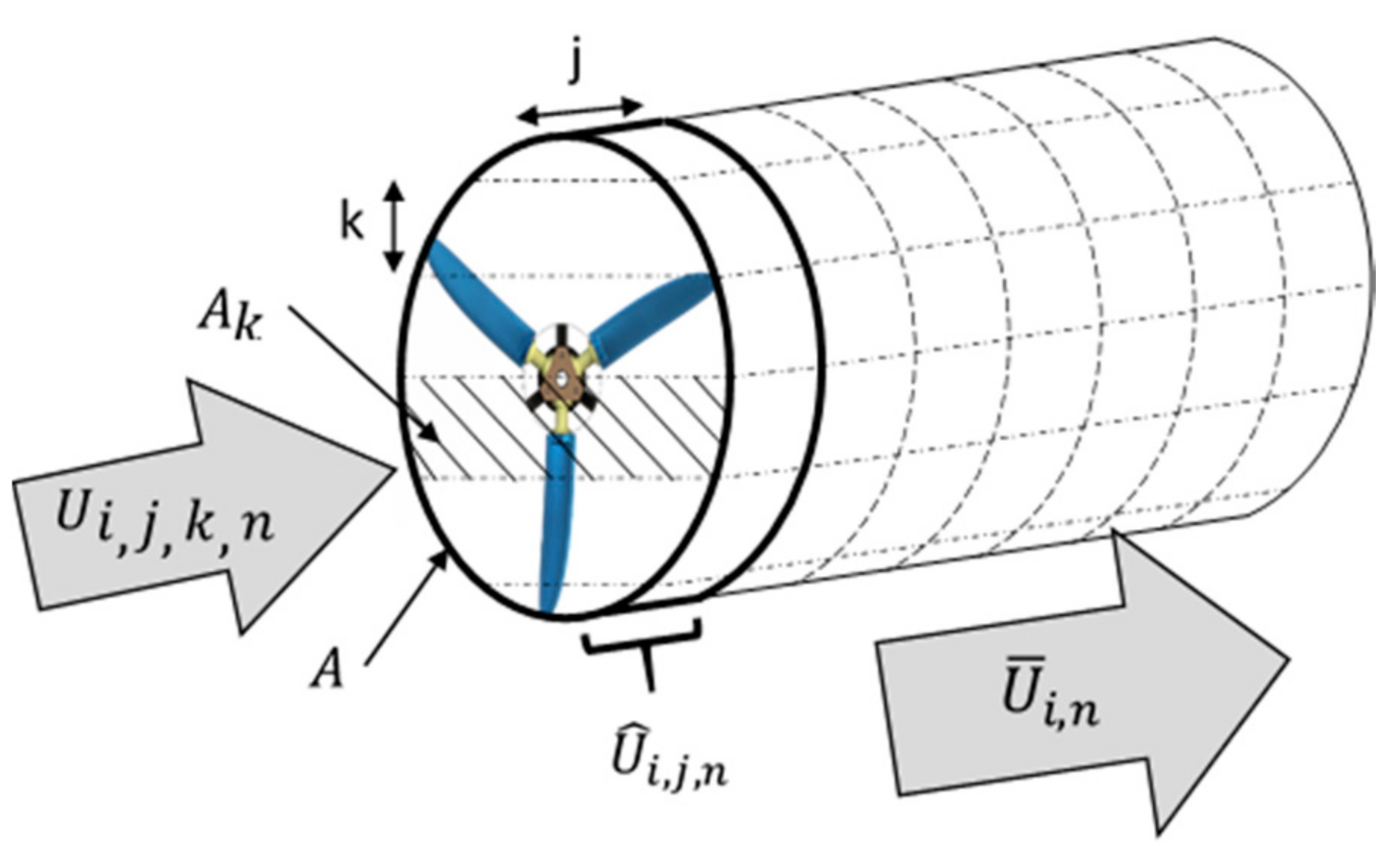
3. Non-Dimensional Performance Characteristics

As previously noted, the DAQ features a National Instrument Compact Rio, the cRio synchronises the various instrument and control data streams into a common format, timestamps them and outputs them as a data file for post-processing.

To compare and analyse the performance of the turbine between the various experimental campaigns, the non-dimensional performance characteristics will be derived. These are shown in Equations (1) and (2) and provide the Tip Speed Ratio (TSR) and Coefficient of Power (C_P).

$${\mathrm{TSR}}_i=\frac{{\overline{\omega }}_i\times r}{{\overline{U}}_i}$$

(1)

$$C_{P,i}=\frac{{\overline{P}}_i}{\frac{1}{2}\times \rho \times A\times {\overline{U}}_i{}^3}$$

(2)

where the rotational speed of the turbine ω was in rad/s, the turbine radius, r = 0.75 m, water density, $\rho =1025 \mathrm{kg}/{\mathrm{m}}^3$ and the turbine area, $A=1.767 {\mathrm{m}}^2$. The mean power, $\overline{P}$ was derived from the product of the rotational speed and mechanical torque measurements averaged over the period of the test window. Both non-dimensional performance indicators require a value for the inflow velocity to the turbine (${\overline{U}}_i$). To derive the mean current velocity, the method of bins, employed by the IEC 62600:200 [23], was used. This method has been outlined in previous work; however, the method has since been developed by the authors to account for bias introduced by the Doppler noise and thus determine the associated uncertainty in the inflow velocity. Further detail on the method and its development can be found in Appendix B and previous research [13].

4. Results

The following section is presented in two subsections, time series results and derived performance (time averaged) results. In each subsection, the comparison between field and lab results will be made and a comparison of the two turbine control strategies (open loop and PID control).

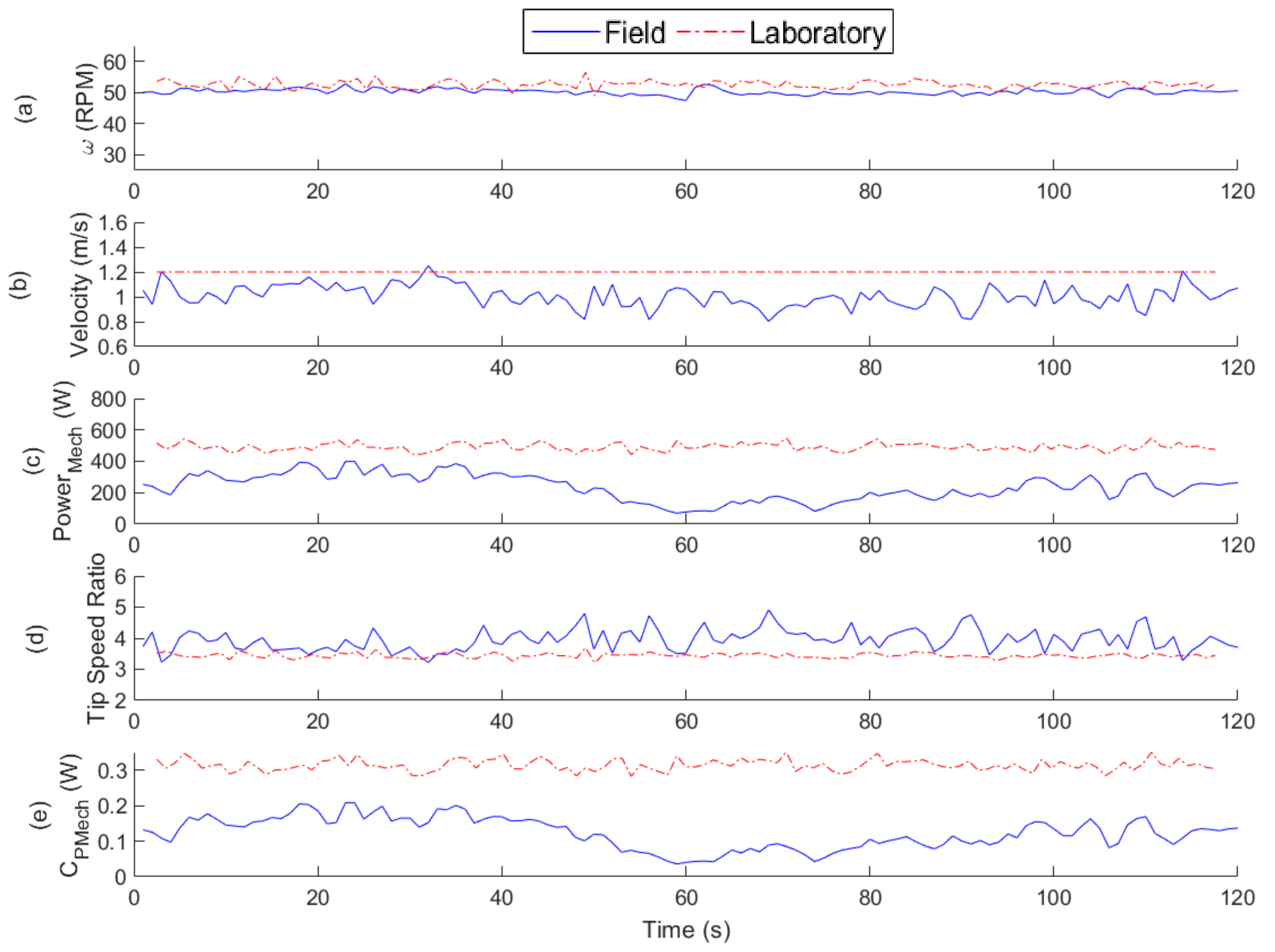
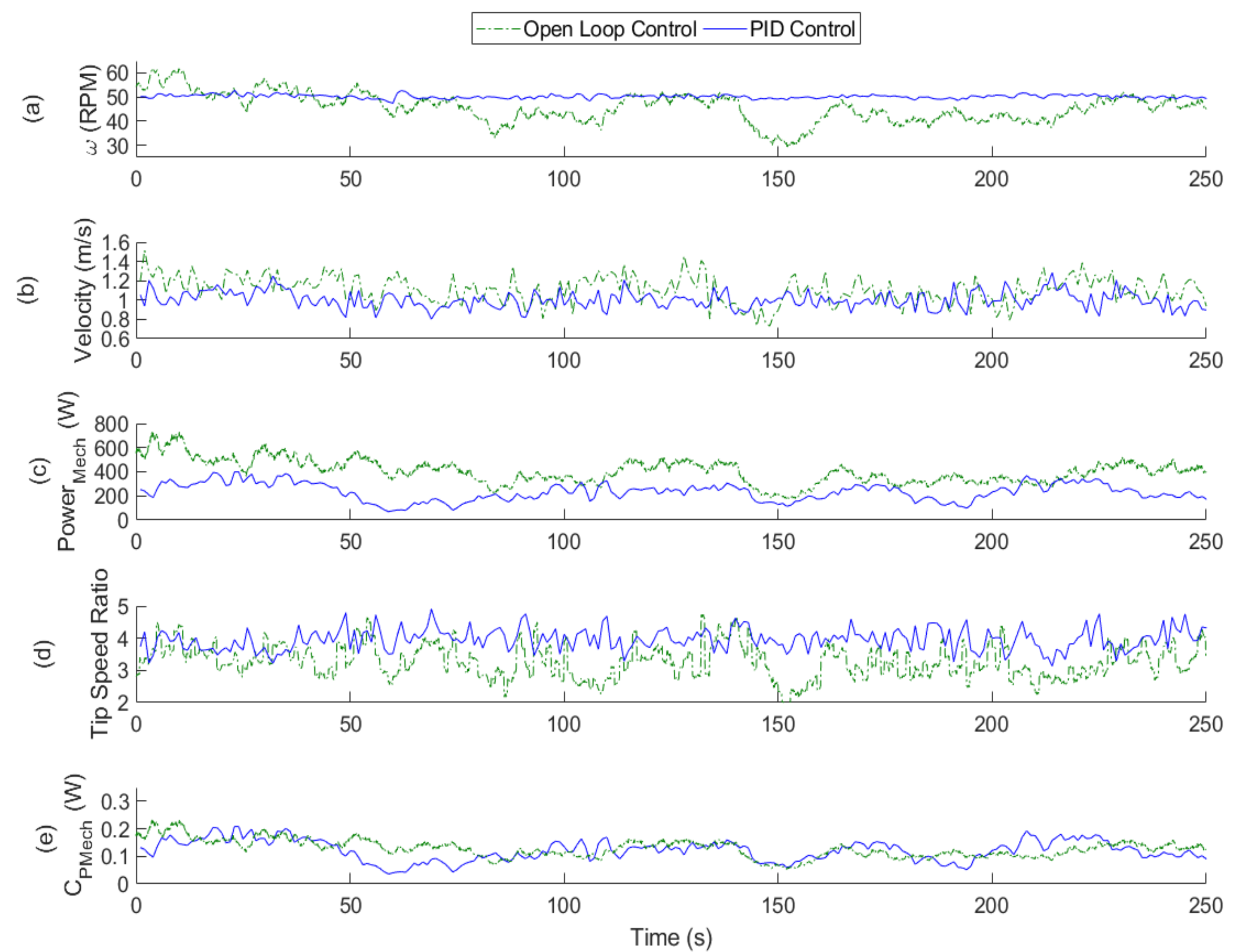
4.1. Time Series Results

Figure 5 is a time series plot comparing the experimental data in the field (Strangford Lough) and the lab (CNR-INSEAN); the two experimental setups feature the PID controller and were conducted under the TTT 3 experiments in 2016/17. Turbine rotational speed, fluid inflow velocity and turbine output power are plotted as time series. Figure 5a shows the rotational velocity from the PID controller was set to 50 RPM for the field and lab. The stability in both sets of results are good with standard deviations of 2σ_RPM = 1.57 and 0.45 respectively for the field and lab. Subplot (b) shows the relative velocity of the water passing the turbine. One of the challenges of ADP and ADV deployments in towing tanks is maintaining a sufficient level of seeding in the water to suit the acoustic reflection and achieve strong SNR, this is not an issue in the field. For the lab velocity, the carriage encoder was used to derive the velocity and subsequent performance characteristics. The ADP results from the field show high flow variation (2σ_Vel = 0.18) and this instability is carried through to the mechanical power of the turbine (see Figure 5c, while the steady conditions in the lab result in a steady power output.

The derived non-dimensional performance characteristics are shown in subplots (d) and (e). For the field results it is clear the TSR fluctuates with the inverse of the inflow velocity as expected. More significantly, the slight difference in TSR results in a significant difference in the C_P. The lab results have a stable TSR and C_P with 2σ_TSR = 0.16 and 2σ_CP = 0.03, while the fluctuating field results have lower mean value and higher standard deviation (2σ_TSR = 0.70 and 2σ_CP = 0.07).

Figure 6 shows the time series results from the open loop controller and PID controller from Strangford Lough field campaigns in TTT and TTT 3. Time series were selected which had the same time-averaged velocity and the time series (and thus average) extends to circa four minutes in both cases. The TTT deployment in 2013 used an open loop control strategy setting a constant demand torque to the alternator, while the TTT 3 deployment in 2016 used the PID (closed loop) control strategy with a set RPM, fluctuating the demand torque to maintain the constant RPM. Note the PID Control case exhibits the same results as shown in Figure 5. The open-loop control RPM time series (Figure 6a) has a higher standard deviation (2σ_RPM = 6.37) than the equivalent closed-loop control time series (2σ_RPM = 1.49). However, maintaining a constant RPM does not result in a constant power output due to the fluctuations in the inflow velocity as shown in Figure 6b. The inflow velocity for both experiments is derived from the IEC method of bins using the ADP data, as described previously. The mechanical power time series, Figure 6c, shows little difference in signal fluctuation between the two control methods, as confirmed by the standard deviations (2σ_Power = 110.58 and 109.88 respectively for open and PID control). The cause of the fluctuations has now been isolated to the inflow velocity fluctuations, as opposed to the type of control strategy, and can be considered independent of fluctuations in RPM. The further significance of these two control strategies can be seen in the derived performance characteristics. Figure 6d,e show the TSR and C_P it is clear that while the PID experiences a more stable TSR value (2σ_TSR = 1.02 and 0.70 Open and PID control respectively) the C_P for both control strategies have similar fluctuations (2σ_CP = 0.06 and 0.07 Open and PID control respectively).

4.2. Derived Performance Results

The power performance characteristics of the Eppler rotor using the same experimental setup and PID control settings in CNR-INSEAN and Strangford Lough are shown in Figure 7. The varying inflow experienced at Strangford Lough has been plotted in the figure using 0.1 ms⁻¹ velocity bins associated with each of the time averaged reading (this is in accordance with the IEC standard [23]). Two trends are noted in to the uncertainty bounds; firstly, with increasing TSR, the uncertainty increases. This indicates the uncertainty from rotational speed, ω and inflow velocity ${\overline{U}}_i$ are the dominating sources. Secondly, the uncertainty bounds for low velocity bins (U_0.8–U_1.0) are comparably greater than higher velocity bins (U_1.1–U_1.4) at the same or similar TSR values. This may be due to the Signal to Noise Ratio (SNR) of the instrument being poor at these lower velocities, increasing uncertainty. The two curves show very close agreement at low TSR; however, as the power curves reach their peak, there is an 8.0% difference in C_P and a 4.5% difference in the TSR for peak C_P. The separation between the curves is maintained as the turbine approaches freewheeling. The uncertainty bounds in the results overlap, but there is also a number of data points well below the performance curve. This deficit in power performance is due to the unsteady inflow parameters and this outcome agrees with Starzmann et al. [11] and is also comparable with results from the flume experiments by Blackmore et al. [15]. This shows that turbine power performance is adversely affected by unsteady inflow. Further consideration of the inflow turbulence metrics and their significance on hydrodynamic performance must be considered.

In its nature, a tidal test site will have a significantly varying inflow, this can be seen by the data points corresponding to the average velocity over which they were taken.

Table 5. Tabulated results for Strangford Lough.

Velocity Bin (ms−1)	Mean Current Velocity, (${\overline{\mathit{U}}}_{\mathit{i}}$)	Mean Power Output, (${\overline{\mathit{P}}}_{\mathit{i}}$)	Mean SD of Power Output, ($\stackrel{´}{{\overline{\mathit{S}\mathit{D}}}_{\mathit{P}}}$)	Number of Data Sets, n
0.65–0.75	0.720	37.972	7.088	3
0.75–0.85	0.802	100.929	45.999	6
0.85–0.95	0.922	113.202	59.554	4
0.95–1.05	1.012	193.498	94.951	13
1.05–1.15	1.100	215.158	91.195	16
1.15–1.25	1.183	264.867	78.834	8
1.25–1.35	1.254	83.518	15.557	2

further shows this variation in velocities in accordance with the IEC standards for power performance of a tidal turbine [23]. Each data set in the velocity bins comes from a time averaged result of at least 2 min.

In Figure 8, the average mechanical power performance of the PID control system can be seen to have a higher performance curve than the equivalent open loop control system. At peak performance, the PID control turbine is 13.7% more efficient than the open-loop control turbine.

In addition to the increase in performance, the inclusion of the closed-loop control system improves the distribution of the data points across the C_P-TSR curve. The open-loop control results have greater scatter, resulting in a comparatively poorer fit (R² = 0.84 and 0.96 for Open and PID Control respectively, Degrees of Freedom = 4). Furthermore, on the right-hand side of the curve, the closed-loop control system has reached a higher TSR, providing a fuller picture of the Eppler rotor performance curve, this is due to the control system having a higher variability in resistance, thus getting closer to freewheeling.

5. Discussion

The comparison of performance in turbine response during experiments in the lab and field show that the performance characteristics do change in the presence of unsteady inflow conditions. While there is a performance drop in C_P between the lines of best fit of the steady lab conditions and the unsteady field conditions, the uncertainty bounds of the data points overlap suggesting the difference is with the region of uncertainty. In order to improve these uncertainty bounds, it is suggested that increasing the number of samples/sample rate or increasing the number of bins in the projected area of the rotor is required. These options are limited when using an ADP due to their correlation with the Doppler noise source. This highlights the importance of instrument selection and setup for deriving the inflow performance.

The method used to account for uncertainties shows robustness in its application in the field and lab. The use of ADPs to measure inflow in the field is appropriate in high flow environments, when characterising full-scale turbine performance, in accordance with the IEC standard. However, awareness of the ADPs’ contribution to uncertainty in the derived performance characteristics is important. Due to the difficulty in maintaining sufficient seeding material in towing tanks, the appropriateness of ADPs remains a challenge; however, as shown in steady flow conditions, the carriage velocity is sufficiently accurate. Alternatively, Particle Image Velocimetry (PIV) measurements would be the favoured method in towing tanks.

The comparison of the PID controller with a set RPM and open-loop controller in unsteady inflow conditions (Strangford Lough) showed a 13.7% difference in peak C_P. The reasons for this distinction in performance are shown in the time series results. Figure 6d shows that restricting the RPM with the PID controller reduces the fluctuation in the TSR over the period of the experiment. As the open-loop control experiences greater fluctuations in TSR, during experiments near peak performance the turbine will be operating at suboptimal TSR in the C_P-TSR curve. This accounts for the reduction in scatter and higher performance at optimal TSR. However, the PID control with set RPM still results in a fluctuating TSR. In a commercial system where characterising the performance curve isn’t the objective, a more appropriate control strategy would use a set TSR, or peak power tracking. This may require knowledge of both the turbine rotational speed and the inflow velocity. This is a consideration for further work.

6. Conclusions

The experimental work presented in this paper successfully completed two experimental campaigns in CNR-INSEAN, Italy and Strangford Lough, Northern Ireland. The continuity of experimental equipment between the two sites provided the opportunity to investigate ADP and ADV calibration agreement with factory settings. It was found that both instruments closely agreed with the factory transformation matrices.

The research has furthered the development of the IEC bin method [23] by the inclusion of a Doppler noise bias correction factor and a method for calculating uncertainties in the derived performance characteristics, with particular attention to uncertainties associated with inflow characterisation.

The work has shown that the effect of unsteady inflow on the derived turbine power performance has a slight detrimental impact of circa 8%. This is in line with the findings of Starzmann et al. [11] and Blackmore et al. [15] and can be considered within the experimental accuracy. To clarify this further will require narrowing the confidence intervals and possible methods of doing this have been suggested.

The two control types, representative of typical strategies in experimental and prototype devices, have shown that a PID feedback controller with set RPM helps achieve a distinctly higher performance curve than the open loop control system, when applied to the turbine operating in unsteady flow conditions such as Strangford Lough. This is critical to consider in experimental design. The fluctuating TSR, as a result of unsteady flow and constrained RPM, remains a weakness in the system if in the presence of large inflow fluctuations. For this reason, it is recognised as a suitable control strategy for characterising a turbine in unsteady flow conditions. Continued development of the PID control is an area of further work, using peak power tracking algorithms and a pre-defined power curve. The inclusion of these strategies will bring the device further in-line with existing industry strategies and make experimental output more relatable to the sector.

References

1. Department for Buisness, Energy & Industrial Stragety. Contracts for Difference Second Allocation Round Results. 2017. Available online: https://www.gov.uk/government/publications/contracts-for-difference-cfd-second-allocation-round-results (accessed on 20 January 2018).
2. Mason-Jones, A.; O’Doherty, D.M.; Morris, C.E.; O’Doherty, T.; Byrne, C.B.; Prickett, P.W.; Grosvenor, R.I.; Owen, I.; Tedds, S.; Poole, R.J. Non-dimensional scaling of tidal stream turbines. Energy 2012, 44, 820–829. [Google Scholar] [CrossRef]
3. Clarke, J.A.; Connor, G.; Grant, A.D.; Johnstone, C.M. Design and testing of a contra-rotating tidal current turbine. Proc. Inst. Mech. Eng. Part A J. Power Energy 2007, 221, 171–179. [Google Scholar] [CrossRef] [Green Version]
4. Gaurier, B.; Germain, G.; Facq, J.V.; Johnstone, C.M.; Grant, A.D.; Day, A.H.; Nixon, E.; Di Felice, F.; Costanzo, M. Tidal energy “Round Robin” tests comparisons between towing tank and circulating tank results. Int. J. Mar. Energy 2015, 12, 87–109. [Google Scholar] [CrossRef] [Green Version]
5. Mycek, P.; Gaurier, B.; Germain, G.; Pinon, G.; Rivoalen, E. Experimental study of the turbulence intensity effects on marine current turbines behaviour. Part I: One single turbine. Renew Energy 2014, 66, 729–746. [Google Scholar] [CrossRef]
6. Jeffcoate, P.; Whittaker, T.; Boake, C.; Elsaesser, B. Field tests of multiple 1/10 scale tidal turbines in steady flows. Renew. Energy 2016, 87, 240–252. [Google Scholar] [CrossRef]
7. Jeffcoate, P.; Elsaesser, B.; Whittaker, T.; Boake, C. Testing Tidal Turbines—Part 1: Steady Towing Tests vs. Tidal Mooring Tests. In Proceedings of the ASRANet International Conference on Offshore Renewable Energy, Glasgow, UK, September 2014; Volume 68, pp. 55–87. Available online: https://pure.qub.ac.uk/portal/files/11366206/ASRANet_2014_PJeffcoate.pdf (accessed on 20 January 2018).
8. Atcheson, M.; MacKinnon, P.; Elsaesser, B. A large scale model experimental study of a tidal turbine in uniform steady flow. Ocean Eng. 2015, 110, 51–61. [Google Scholar] [CrossRef] [Green Version]
9. Jeffcoate, P.; Salvatore, F.; Boake, C.; Elsaesser, B.; Vallerano, V. Effect of Submergence on Tidal Turbine Performance. In Proceedings of the 11th European Wave and Tidal Energy Conference, Nantes, France, 6–11 September 2015; pp. 3–9. [Google Scholar]
10. Jeffcoate, P.; Starzmann, R.; Elsaesser, B.; Scholl, S.; Bischoff, S. Field measurements of a full scale tidal turbine. Int. J. Mar. Energy 2015, 12, 3–20. [Google Scholar] [CrossRef] [Green Version]
11. Starzmann, R.; Jeffcoate, P.; Scholl, S.; Bischof, S.; Elsaesser, B. Field testing a full-scale tidal turbine Part 1: Power Performance Assessment. In Proceedings of the 11th European Wave and Tidal Energy Conference, Nantes, France, 6–11 September 2015; pp. 1–7. [Google Scholar]
12. Schmitt, P.; Elsaesser, B.; Bischof, S.; Starzmann, R. Field testing a full-scale tidal turbine Part 2: In-line Wake Effects. In Proceedings of the 11th European Wave and Tidal Energy Conference, Nantes, France, 6–11 September 2015; pp. 1–7. [Google Scholar]
13. Frost, C.; Benson, I.; Elsäßer, B.; Starzmann, R.; Whittaker, T. Mitigating Uncertainty in Tidal Turbine Performance Characteristics from Experimental Testing. In Proceedings of the European Wave & Tidal Energy Conference, Cork, Ireland, 27 August 2017. [Google Scholar]
14. Forbush, D.; Polagye, B.; Thomson, J.; Kilcher, L.; Donegan, J.; McEntee, J. Performance characterization of a cross-flow hydrokinetic turbine in sheared inflow. Int. J. Mar. Energy 2016, 16, 150–161. [Google Scholar] [CrossRef] [Green Version]
15. Blackmore, T.; Myers, L.E.; Bahaj, A.S. Effects of turbulence on tidal turbines: Implications to performance, blade loads, and condition monitoring. Int. J. Mar. Energy 2016, 14, 1–26. [Google Scholar] [CrossRef] [Green Version]
16. European Commission Technology readiness levels (TRL). Horizon 2020 General Annexes; European Commission: Brussels, Belgium, 2015; p. 4995. [Google Scholar]
17. Mason-Jones, A.; O’Doherty, D.M.; Morris, C.E.; O’Doherty, T. Influence of a velocity profile & support structure on tidal stream turbine performance. Renew. Energy 2013, 52, 23–30. [Google Scholar] [CrossRef]
18. Payne, G.S.; Stallard, T.; Martinez, R. Design and manufacture of a bed supported tidal turbine model for blade and shaft load measurement in turbulent flow and waves. Renew. Energy 2017, 107, 312–326. [Google Scholar] [CrossRef]
19. Harrold, M.J. Experimental and Numerical Assessment of a Tidal Turbine Control Strategy, University of Strathclyde, 2016. Available online: http://ethos.bl.uk/OrderDetails.do?uin=uk.bl.ethos.723008 (accessed on 20 January 2018).
20. Allmark, M.; Grosvenor, R.; Prickett, P. An approach to the characterisation of the performance of a tidal stream turbine. Renew. Energy 2017, 111, 849–860. [Google Scholar] [CrossRef]
21. Schlipf, D.; Pao, L.Y.; Cheng, P.W. Comparison of Feedforward and Model Predictive Control of Wind Turbines Using LIDAR. In Proceedings of the 2012 IEEE 51st IEEE Conference on Decision and Control (CDC), Maui, HI, USA, 10–13 December 2012; pp. 3050–3055. [Google Scholar]
22. Johnstone, C.M.; McCombes, T.; Bahaj, A.S.; Myers, L.E.; Holmes, B.; Koefoed, J.P.; Bittencourt, C. EquiMar: Development of Best Practices for the Engineering Performance Appraisal of Wwave and Tidal Energy Converters. In Proceedings of the 9th European Wave and Tidal Energy Conference, Southampton, UK, 5–9 September 2011. [Google Scholar]
23. IEC/TS 62600-200 Power Performance Assessment of Electricity Producing Tidal Energy Converters Commissioned by: IEC. 2011. Available online: https://webstore.iec.ch/publication/7242 (accessed on 20 January 2018).
24. Clark, T.; Black, K.; Ibrahim, J.; Minns, N.; Fisher, S.; Roc, T.; Hernon, J.; White, R. MRCF-TiME-KS9b Turbulence: Best Practices for Data Processing, Classification and Characterisation of Turbulent Flows. Ocean Array Systems: Edinburgh, UK. 2015. Available online: http://www.oceanarraysystems.com/publications (accessed on 20 January 2018).
25. Shih, H.H.; Payton, C.; Sprenke, J.; Mero, T. Towing Basin Speed Calibration of Acoustic Doppler Current Profiling Instruments. In Joint Conference on Water Resource Engineering and Water Resources Planning and Management 2000; American Society of Civil Engineers: Reston, VA, USA, 2000; pp. 1–10. [Google Scholar]
26. Oberg, K.; Mueller, D.S. Validation of Streamflow Measurements Made with Acoustic Doppler Current Profilers. J. Hydraul. Eng. 2007, 133, 1421–1432. [Google Scholar] [CrossRef]
27. Elsaesser, B.; Torrens-Spence, H.; Schmitt, P.; Kregting, L. Comparison of Four Acoustic Doppler Current Profilers in a High Flow Tidal Environment—Queen’s University Belfast Research Portal—Research Directory & Institutional Repository for QUB. In Proceedings of the 3rd Asian Wave and Tidal Energy Conference, Singapore, 24–28 October 2016. [Google Scholar]
28. Pao, L.Y.; Johnson, K.E. Control of Wind Turbines. IEEE Control Syst. 2011, 31, 44–62. [Google Scholar] [CrossRef]
29. Bennett, S. The past of pid controllers. Annu. Rev. Control 2001, 25, 43–53. [Google Scholar] [CrossRef]
30. Ziegler, J.G.; Nichols, N.B. Optimum Settings for Automatic Controllers. J. Dyn. Syst. Meas. Control 1993, 115, 220. [Google Scholar] [CrossRef]
31. Haldane, J.B.S. Moments of the distributions of power and products of normal variates. Biometrika 1942, 32, 226–242. [Google Scholar] [CrossRef]
32. Doman, D.A.; Murray, R.E.; Pegg, M.J.; Gracie, K.; Johnstone, C.M.; Nevalainen, T. Tow-tank testing of a 1/20th scale horizontal axis tidal turbine with uncertainty analysis. Int. J. Mar. Energy 2015, 11, 105–119. [Google Scholar] [CrossRef]
Figure 1. Tidal Turbine Testing (TTT) device and rotor.
Energies 11 01533 g001
Figure 2. Turbine, Acoustic Doppler profiler (ADP) and Acoustic Doppler Velocimetry (ADV) deployment Configuration.
Energies 11 01533 g002
Figure 3. TTT 2 open-loop control and binary load.
Energies 11 01533 g003
Figure 4. TTT 3 closed-loop Proportional–Integral–Derivative (PID) control and programmable load.
Energies 11 01533 g004
Figure 5. Time series plot of (a) turbine rotational speed; (b) inflow velocity; and (c) mechanical power. (d) Tip Speed Ratio and (e) Coefficient of Mechanical Power using PID controller in the lab and field.
Energies 11 01533 g005
Figure 6. Strangford Lough time series plot of (a) turbine rotational speed; (b) inflow velocity; and (c) mechanical power. (d) Tip Speed Ratio (e) Coefficient of Mechanical Power.
Energies 11 01533 g006
Figure 7. Mechanical Power performance for Eppler Rotor in the lab and field using PID Controller.
Energies 11 01533 g007
Figure 8. Mechanical Power Performance of turbine in Strangford Lough using two control strategies.
Energies 11 01533 g008