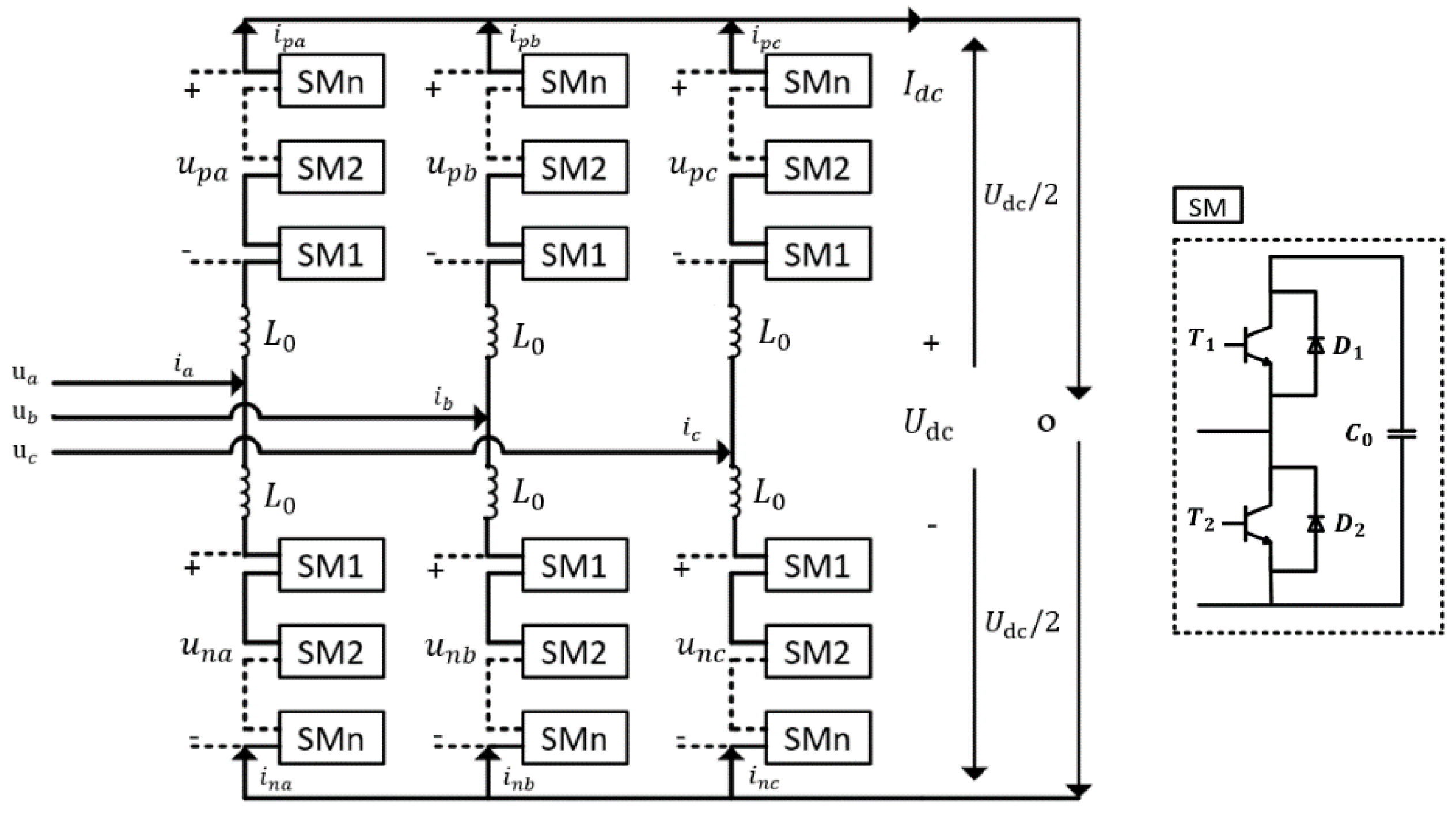
Article

Rapid Fault Diagnosis of a Back-to-Back MMC-HVDC Transmission System under AC Line Fault

1
School of Electrical Engineering, Wuhan University, Wuhan 430072, China
2
State Grid Energy Conservation Service Co., Ltd., Beijing 100052, China
*
Author to whom correspondence should be addressed.
Energies 2018, 11(6), 1534; https://doi.org/10.3390/en11061534
Submission received: 12 May 2018 / Revised: 5 June 2018 / Accepted: 11 June 2018 / Published: 12 June 2018
(This article belongs to the Section F: Electrical Engineering)

Abstract

:
The integration of a modular multilevel converter-based high-voltage direct current (MMC-HVDC) transmission system in power networks has led to a high requirement for the rapidity of fault recognition. This study focused on the rapid fault diagnosis of an alternating current (AC) line fault in a back-to-back (BTB) MMC-HVDC system via fault detection and classification. Discrete wavelet transform and modulus maxima were applied to extract the fault features. Phase-mode transformation and normalization were adopted to widen the application range. Simulation and calculation results indicated that the proposed method can detect all fault types in an AC transmission line on the basis of single-side fault information within 1 ms under different values of transition resistance, fault inception angle, and fault distance. The BTB MMC-HVDC model was built using real-time laboratory (RT-LAB) based on the matrix laboratory (MATLAB) software platform, and the fault diagnosis algorithm was performed in MATLAB.

1. Introduction

Owing to the weakness of electronic devices in modular multilevel converter-based high-voltage direct current (MMC-HVDC) transmission systems, the required fault detection time is considerably lower in these systems than in AC transmission systems to prevent damage to electronic components caused by overcurrent scenarios. Several mitigation schemes, such as increasing the bridge inductance and changing the circuit structure, have been proposed to save extra time for the fault relay. However, fault diagnosis, as the first step in fault protection in the MMC-HVDC, still requires a faster method than existing detection methods.
Previous work on MMC-HVDC has mainly concentrated on analyzing fault characteristics via calculations and simulations [1,2,3,4] and on control strategies under fault conditions [5,6,7,8]. The fault in an AC/DC (direct current) hybrid system is simulated by comparing different fault features [1]. A single phase-to-ground fault on the AC side is studied from a dynamic process perspective, and second-order harmonics that appeared in the DC voltage are attributed to a negative sequence component [2,3]. Similarly, the AC fault of an AC/DC hybrid network has been analyzed in relaying the angle, summarizing the fault pattern of the harmonics component, and revealing sequence impedance [3]. Faults at the AC, DC, and valve sides of the MMC-HVDC system and the corresponding fault transient simulations are performed considering different transformer connections [4]. On the basis of fault analysis, corresponding control strategies are proposed to maintain system stability [5,6,7,8]. The fault detection method in an AC transmission line cannot be directly applied to the fault diagnosis of the MMC-HVDC system given different topologies and fault protection requirements. The AC transmission line fault detection time in previous approaches [9,10,11,12,13] exceeds 2.5 ms, which cannot satisfy the protection requirement of the MMC-HVDC system. Renyi wave packet energy entropy (RWPEE) is adopted to extract fault transient features; RWPEE strategy is suggested to detect faults in the future scope [14] and is performed in Reference [15]. A hybrid topology has been presented in reference [16], which includes half-bridge (HB) and full-bridge (FB) submodules to facilitate circuit breaker operation under a single phase-to-ground fault at the valve side of the MMC-HVDC system. Thus, detecting AC faults in the MMC-HVDC must be further explored.
This study focuses on the rapid AC line fault detection and fault phase selection of the MMC-HVDC via fault characteristic analysis and simulation validation. Among the existing fault detection methodologies in voltage source converter-based high-voltage direct current (VSC-HVDC) transmission systems and conventional AC transmission lines, wavelet analysis is universally applied, especially in combination with entropy theory [14,16,17,18,19,20], and a boundary condition is applied to distinguish internal from external faults [17,21,22,23]. An artificial neural network [24] and machine learning [25,26] are utilized to train the proposed fault detection model or algorithm for improved accuracy. As mentioned in Reference [27], previous protection schemes in AC systems cannot be directly applied to an AC/DC hybrid system because of the different pattern in fault current characteristics between AC systems and AC/DC hybrid systems. Therefore, a back-to-back (BTB) MMC-HVDC model based on the actual BTB-HVDC project [28] is built to examine fault diagnosis.
The remainder of this paper is organized as follows. Fault analysis is described in Section 2. Based on the fault characteristics, the fault detection theory and classification scheme are demonstrated in Section 3 and Section 4, respectively. Section 5 presents the fault simulation results to verify the reliability and accuracy of the proposed method. The relevant discussion and drawn conclusion are provided in Section 6.

2. Fault Analysis

2.1. Working Principle

The MMC involves three phase units with six arms. Each arm consists of several sub-modules (SM) and equivalent inductance L 0 in series. Each phase unit has an upper and a lower arm, as illustrated in Figure 1. In each SM, the switch T 1 and T 2 are controlled by a modulation signal, which contributes to the output of each arm, to charge or discharge. The output waveform of each phase unit is determined by the upper and lower arms.
The AC input voltage and current of the converter are u j and i j (j = a, b, c), respectively. U d c and I d c are the DC link voltage and current. The voltages of the upper and lower arms are u p j and u n j (j = a, b, c), respectively. The arm currents are i p j and i n j (j = a, b, c), and o is the neutral point for voltage reference.
According to Kirchhoff current theory, the AC input phase current i j can be described as
i j = i p j i n j , j = a , b , c
In each phase unit, the arm current is expressed as [14]
i j d i f = i p j i n j 2 , j = a , b , c
In accordance with the topology depicted in Figure 1, the currents in the upper and lower arms of each phase unit are presented as
i p j = i j 2 + I j d c + i j a c , j = a , b , c
i n j = i j 2 I j d c i j a c , j = a , b , c
where I j d c and i j a c are the DC and AC components in the arm current. The following equations can be obtained in accordance with Kirchhoff voltage theory:
u j ( U dc 2 u p j ) = L 0 d i p j d t , j = a , b , c
u j ( U dc 2 + u n j ) = L 0 d i n j d t , j = a , b , c
Thus, adding Equations (5) and (6) results in Equation (7).
u j u n j u p j 2 = L 0 d i j d t , j = a , b , c
The subtraction of Equation (6) from Equation (5) yields
U d c = ( u p j + u n j ) L 0 d i j a c d t , j = a , b , c
The DC link current can be expressed as
I d c = j = a , b , c ( I j d c + i j a c )
The dynamic characteristics of the DC side in the MMC are defined using Equations (8) and (9), which can be utilized under normal condition and fault analysis.

2.2. Fault Simulation

The BTB MMC-HVDC model is displayed in Figure 2, and the system parameter settings are listed in Table 1. The fault investigation in this study focused on the AC line section at the rectifier side called fault F1, as exhibited in Figure 2. The control strategies of converter adopted in this model are constant active power and reactive power control (rectifier) and constant DC voltage and reactive power control (inverter). The single-line grounded (SLG) fault was simulated in the BTB-HVDC model built using RT-LAB (11.0) and MATLAB (2011b). The fault transients of the AC side is demonstrated in Figure 3.
In Figure 3b, the difference between fault phase currents and sound phase currents is not obvious, and the fault detection time used in the phase current amplitude-based method can reach a 1/4 cycle given the varying fault inception angles. In addition, power electronic devices are vulnerable under fault due to overcurrent and therefore require a rapid fault detection method to protect them from breaking.
In a real BTB-HVDC project, the current measurement points are set at the entrance of the converter, the arms, and the DC link. In Figure 2, the phase current at point M—that is, the entrance of the rectifier—is detected and analyzed as the fault signal. AB-phase ungrounded and AB-phase grounded (ABG) short-circuit faults are simulated using MATLAB. The three phase currents in (a) and (b) are nearly the same and cannot be directly used as the fault current at point M (Figure 4) to detect grounded faults. Furthermore, It is highlighted that the sound phase current in a two-phase grounded short-circuit fault is not constantly low in current amplitude [29]. Therefore, the fault component of the phase current at M can be a favorable choice for fault detection. According to the superposition principle, the transmission system under a short-circuit fault can be considered as a normal state with an additional fault state. Thus, the fault current I f can be divided into the normal operation component i normal and the fault component i f . The normal operation and fault components use the fault and sound phase currents under the ABG fault as an example (Figure 5). The fault component denoted by the green line depicts the distinguished patterns in the fault and sound phases.

2.3. Fault Calculation

A phase-A grounded (AG) short-circuit fault is used as an example, and the fault components of the fault current in each phase are calculated on the basis of the equivalent circuit presented in Figure 6. R 1 and L 1 are the equivalent resistance and inductance of the grid-side loop, which involves zero- and negative-sequence components. A similar rule is applied to the converter-side loop with subscript 2. R g denotes the grounded resistance.
In the grid-side loop,
L 1 d i 1 d t + R 1 i 1 = U max cos ( ω t + ϕ u )
i 1 = U max | Z | cos ( ω t + ϕ u φ ) U max | Z | cos ( ϕ u φ ) e t / τ
| Z | = ( R 1 + R g ) 2 + ω 2 L 1 2
τ = L 1 / ( R 1 + R g )
φ = arccos ( ( R 1 + R g ) / | Z | )
In the converter-side loop,
C e q L 2 d 2 u c d t 2 + R g L 2 d u c d t + u c = 0
i 2 = U d c ω c L 2 e δ t sin ( ω c t )
δ = R g + R 2 2 L 2
ω c = 1 C e q L 2 δ 2
According to the calculation results, the fault component consists of a fundamental frequency fault component, a damped AC component, and a damped DC component. The simulation and calculated values of the AG fault phase currents are illustrated in Figure 7. The fault components under the other fault types can be calculated by using a similar approach.

3. Fault Diagnosis Theory

The fault signal of phase current has been processed with phase module transform in the first step, because the electromagnetic coupling effect might influence the fault detection result. In order to realize the fault detection and fault classification, the wavelet transform has been adopted to reflect fault signal in the time-frequency domain. Moreover, the modulus maxima of each phase current signal under multi-resolution decomposition has been chosen to indicate fault time and fault phase. The techniques involved in the proposed method is explained in detail below.

3.1. Phase Module Transform

A phase-module transform is adopted to eliminate the mutual influence among transmission lines given the electromagnetic coupling in the three-phase transmission line. In contrast to previous studies [18,30], the fault component of the fault current is transformed via Clark transform. 0 and α moduli are obtained to decouple the three-phase fault components. The phase module transformation matrix is expressed as
[ I a I b I c I 0 ] = [ 2 1 1 1 1 2 1 1 1 1 2 1 ] [ i a i b i c ]
where i a ,   i b ,   and   i c are the three phase currents at the entrance of the rectifier. I a ,   I b ,   and   I c are the α modulus of each phase current, and I 0 is the 0 modulus of the fault phase current.

3.2. Wavelet Transform Theory

Wavelet transform can perform a multi-level resolution on the time and frequency domains and can capture local features better than Fourier transform. Different to the Fourier transform, the window in wavelet transform has an adjustable window to decompose the signal in both high and low frequency resolutions with different decomposition scales. The most important aspect is that wavelet transform is very sensitive to a singular point in the signal. Thus, the wavelet transform can be adopted to analyze the high-frequency fault signal [30].
Wavelet analysis requires a mother wavelet, whose precondition is
Ψ ( t ) L 2 ( R )
+ | Ψ ( t ) | ω d ω < +
where L 2 (R) in Equation (20) represents a square-integrable real number region, and Ψ ( ω ) in Equation (21) is the Fourier transform of Ψ ( t ) . The mother wavelet can be scaled and shifted using Equation (22) with the shift parameter τ and the scale parameter a .
Ψ a , b ( t ) = 1 a Ψ ( t τ a ) d t , τ R , a > 0
Continuous wavelet transform is defined as Equation (23) with f ( t )   L 2 ( R ) .
W a τ f ( t ) = | a | 1 / 2 + f ( t ) Ψ ( t τ a ) d t
where Ψ ( t ) denotes a complex conjugate. Discrete wavelet transform is typically used in real applications and can be defined as Equation (24) with a   =   2 j ,   k   =   2 j τ ,   j ,   k     Z .
W j k f ( t ) = | 2 | 1 / 2 + f ( t ) Ψ ( 2 j t k ) d t

3.3. Multi-Resolution Signal Decomposition (MSD)

A given signal or image can be decomposed into detailed and approximated versions via the MSD [31] technique. The original signal can be decomposed into signals of different frequency bands by applying the Mallat algorithm.
The assumption is that the original signal f ( t ) is decomposed under the j-level (j = 1, 2, 3…); f ( t ) can be expressed as Equation (25).
f ( t ) = A j f ( t ) + j = 1 J D j f ( t )
where A j   f ( t ) is the approximate signal on the j-level decomposition scale within the frequency band ( 0 ,   2 j ) . D j f ( t ) is the detail signal on the j-level decomposition scale within the frequency band ( 2 j ,   2 j + 1 ) .

3.4. Modulus Maxima

In the discrete wavelet transform depicted in Equation (15), if the time point t 0 ( j ,   k ) satisfies Equations (26) and (27), then
( W j k f ( t 0 ) ) t 0 = 0
| W j k f ( t x ) | | W j k f ( t 0 ) |
where t x is any point in the time region that involves t 0 , and t 0 is the point at which to obtain the modulus maxima under the j-level decomposition. The appearance of modulus maxima indicates the singular point in the fault signal, namely the fault time point. The sign of modulus maxima indicates the signal change direction, and its absolute value reflects the signal change degree. Therefore, the modulus maxima is a promising approach to detecting the fault signal and fault time point.

3.5. Theory Application

The theories mentioned above are applied in fault diagnosis method in a logical flow. Firstly, the phase-module transform is applied to change the phase current to α module and 0 module via the transformation matrix shown in (19). Then, the α module and 0 module are processed with discrete wavelet transform, which is performed in multi-resolution signal decomposition (MSD) to obtain approximate signal A j and detailed signal D j under different decomposing scales, shown in Equation (25). After that, modules maxima are picked up in the detailed signal with Equations (26) and (27). The time point location of modulus maxima indicates that the fault occurrence and modulus maxima amplitude denote the singularity degree of the modulus. In summary, the details of proposed scheme has been demonstrated in Section 4.

4. Fault Detection and Classification Scheme

4.1. Fault Detection

In this study, the modulus maxima of the fault components are adopted to detect the fault time. The AG fault is simulated to clarify the fault detection process, which is exhibited in Figure 8. The fault component of the phase-A current i f a is decomposed with the “db4” mother wavelet in one level to identify the fault time point. The sampling frequency in the simulation is 10 kHz, which is within the sampling frequency range in the real project. The AG fault has occurred at 1.25 s, and the fault time point displayed in Figure 8b,c is at sampling point 100. Figure 8 demonstrates that the decomposition by wavelet transform can perform an acceptable approximation of the original signal and rapidly detect any signal change. The fault is detected on the basis of the maximum detail coefficient (102, 9.405) within 0.2 ms, exhibited in Figure 8c. A similar pattern can be observed in the sound phase current signal in Figure 8f, in which the modulus maxima appeared at (102, −4.758). Therefore, the fault and sound phase current signals can be used to detect the fault within 0.2 ms.

4.2. Fault Classification

The mode fault currents under the boundary condition of different fault types are summarized in Table 2. The fault types in left-side column include single-phase grounded fault (AG,BG,CG), two-phase grounded fault (ABG,ACG,BCG), two-phase ungrounded short circuit fault (AB,AC,BC), three-phase grounded fault (ABCG) and three-phase ungrounded short circuit fault (ABC).
The mode fault currents are replaced by mode fault components to avoid the influence of normal-state components in the calculation of the maximum modulus. M 0 ,   M a ,   M b ,   and   M c are the modulus maxima of the mode fault components I 0 ,   I a ,   I b ,   and   I c . Normalization is performed on the maximum modulus to adapt to a different system operation mode, which was obtained using σ i   =   M i / | max (   M 0 ,   M a ,   M b ,   M c ) | ,   i   =   0   ,   a   ,   b ,   c . The fault types are distinguished by the criterion factor σ i . The entire process for obtaining the criterion factor σ i is displayed in Figure 9. In accordance with the calculation of the fault component in Section 2.2, the different lengths of data are tested to obtain the criterion factor, and the results are presented in Table 3. The results suggest that 1 ms-long data can distinguish fault types on the basis of the criterion factor. The 1 ms-long fault simulation data are applied in the same algorithm, and the results are provided in Table 4, thereby confirming that a 1 ms-long fault component signal can satisfy the proposed scheme requirement.
According to the simulation results in Table 3 and the modulus characteristics under different faults in Table 2, fault classification can start with the criterion factor σ 0 of the 0 modulus. If σ 0 = 0 , then the fault must involve a three-phase fault and a two-phase short-circuit fault, whereas if   σ 0 0 , then the fault must be confined to a single- or a double-phase grounded fault. The auxiliary threshold of the criterion factor is set for a single-phase grounded fault to consider the deviation. In addition, the σ 0 of the double- and triple-phase faults is less than 0.0001, which was rounded to 0. The detailed fault classification scheme is illustrated in Figure 10. In the single-phase grounded fault, the criterion factor of the sound phases is approximately 0.5. Thus, the upper threshold σ 1 m a x and the lower threshold σ 1 m i n are set to 0.52 and 0.48, respectively, considering the fluctuation due to variation in fault condition, in the initial step. In the double-phase short-circuit fault, the threshold of the middle criterion factor σ 2 m a x is set to 0.95, and the threshold of the smallest criterion factor σ 2 m i n is set to 0.05.

4.3. Application of Proposed Scheme

According to the fault detection and classification scheme demonstrated in Section 4.1 and Section 4.2, the basic principle of the proposed method is to define the threshold of criterion factors based on a large amount of tests. However, in the actual protection scheme design, the threshold setting should consider many factors, such as the fault inception angle, fault resistance and fault location. Additionally, the parameters of system components (grid system, transformer and transmission line, etc.), the control mode of the converter station and load variation might affect the fault diagnostic results. Therefore, the corresponding simulation given different factors has been performed to find if the value of criterion factors can be used to distinguish fault types.

5. Simulation Result

5.1. Fundamental Simulation Result

The different faults of F1 demonstrated in Figure 2 are simulated with the corresponding criterion factor results. The sampling frequency is set to 10 kHz, and “db4” mother wavelet and one-scaled wavelet transform are adopted. A 210 sample-long sequence (i.e., 1 ms-long data after fault inception plus a whole cycle data before fault inception) is selected for fault classification. Only the 1 ms-long data are used in the fault classification because the whole cycle data before fault occurrence are considered as the normal-state data for obtaining the fault component. The 21 ms-long sampling window is slid in a step of 0.1 ms. The test results for the different conditions of fault types, resistance, distance from the bus, and inception angle are shown in Figure 11 and Figure 12 and Table 5, Table 6 and Table 7. The dashed lines in figures indicate the upper limit and lower limit of range of criterion factor, which is labeled with corresponding value on vertical axis of figures.
  • Fault classification for various inception angles: The fault cases with various fault inception angles that range from 0 to 2π with a step of π/10 (Figure 11 and Table 5) confirm that the proposed scheme can correctly classify the faults with the appropriate adjustment of the criterion factor threshold. For example, in Figure 11a, σ b and σ c are limited to the range of 0.4788–0.5234. The criterion factor range of sound phase current under single phase grounded fault is wider than that in initial step (Section 4.2).
  • Fault classification for various fault locations: The total AC line length is 200 km, and the fault distance from the bus in the fault cases ranges from 10 km to 190 km with a step of 10 km. The results presented in Table 6 and Figure 12 have confirmed that the proposed fault classification scheme is immune to fault locations.
  • Fault classification for varying fault resistance: In this part, faults with high resistance and metallic short-circuit faults are simulated. The characteristics of each criterion factor exhibit the same pattern as the results demonstrated in Table 7, thereby suggesting that the fault with high resistance can still be detected and classified.

5.2. Supplementary Simulation Result

  • The faults on the DC link of the BTB-HVDC are simulated to determine if the DC-side fault affects the accuracy of the proposed fault classification scheme. In Figure 2, F2 denotes the single pole-to-ground fault. The sign behind F2 in Table 8 indicates the fault pole (“+” positive pole, “−“ negative pole), and F3 denotes the pole-to-pole fault. In the single pole-to-ground fault, the voltage reference point is changed to a fault point, thus increasing the absolute value to the AC-side voltage without destroying the AC-side current stability. Thus, the criterion factor of each phase modulus is approximately 0. However, σ 0   =   1 indicates that the grounding current dominates the fault current in such a scenario. The pole-to-pole fault on the DC side can be equivalent to the AC side three-phase short-circuit fault given the same topology structure under fault. Consequently, the simulation result shows a similar pattern to that of the ABC fault in the previous tests. The detailed results are displayed in Table 8.
  • The faults on the other side (inverter side) are simulated, and the results are presented in Table 9 and Figure 13. The rectifier-side current is unaffected by the inverter-side faults, except for the three-phase short-circuit fault. The current waveforms illustrated in Figure 13a–c are nearly the same as those under the normal operation. In Table 9, the criterion factors under the BC-phase short-circuit fault and ABC phase are likely to be mistaken as the rectifier-side fault. However, the fault detection step fails to identify any obvious jump or decline in the detail fault signal. Moreover, the normal operation cannot be mistaken as a three-phase fault for the same reason. Therefore, the proposed fault detection and classification scheme is feasible under the inverter-side faults and normal operation.
  • Considering the different control modes on the converter station, the current at measuring point M might be influenced, which could affect the fault diagnostic results. Thus, the conventional control modes, including constant active power and reactive power control (PQ control), and constant DC voltage and reactive power control ( V d c Q control), are adopted to investigate the influence on phase current measured at point M. The measured currents under two converter control modes are compared in Figure 14. It can be found that the converter control mode does influence the fault phase current. Therefore, in order to check the feasibility of proposed fault diagnosis scheme, fault case study has been performed under V d c Q control mode. The test result of fault diagnosis method under V d c Q control mode is provided in Table 10 with the same fault condition in Table 4, which indicates the feasibility of proposed fault diagnosis scheme with different converter control mode.
  • The fault current measured at M point would be changed with load variations, which might affect the fault diagnostic result. The experiments considering variation of active power and reactive power have been performed and the results in Table 11 indicates that the proposed method is immune to load change.
  • The parameters of gird system and transformer could influence the fault current, which might affect diagnostic results. Firstly, the short-circuit ratio of gird system is set as 1 and 5 in the contrast test given the unexpected performance of the previous fault detection method on the weak grid system side. Meanwhile, the power flow direction is reversed in contrast test. Secondly, the frequency of two grids in BTB-HVDC model is changed to 49.8 Hz and 50.2 Hz to investigate if frequency fluctuation modifies the diagnostic results. Additionally, the winding resistance, leakage inductance, magnetization resistance and inductance are altered in simulation test. The related results are shown in Table A1, Table A2, Table A3, Table A4 and Table A5 in Appendix A given the length of this paper. It is indicated from the test result that the parameters change in the grid system and that the transformer does not influence the fault diagnostic result of the proposed method in this paper.

5.3. Summary

Based on the simulation results described in this section, it can be found that the criterion factors are in different patterns under different fault scenarios. For example, in the single phase grounded fault, the criterion factor of faulted phase is always 1 and that of the other two sound phases are approximately 0.5; in double-phase grounded fault and ungrounded fault, the criterion factor of the faulted phases is equal to 1 or close to 1, and that of the sound phase is close to 0. Additionally, the criterion factor of 0 modulus can be adopted to distinguish single-phase grounded fault and double-phase grounded fault from the rest because it indicates unbalanced grounded fault. Thus, the proposed scheme could be utilized to detect and classify faults with proper criterion factor threshold setting due to the distinguishable pattern of the criterion factor, and the threshold could be obtained from preparation test considering the factors mentioned in this section.

6. Conclusions

In this study, the characteristics of AC line faults are investigated in a two-terminal BTB-HVDC system, and a fault detection and classification method is proposed. The feasibility of the proposed method is verified by performing numerous simulation tests, which revealed that such a method can detect faults within 0.2 ms and classify AC line fault types within 1 ms. Moreover, a discrete wavelet transform is adopted and incorporated in fault transient signal processing as a commonly applied tool with the concept of modulus maxima to verify that the traditional approach for an AC transmission line fault detection can be used for hybrid AC/DC networks. Remarkable calculation and communication between the two converter stations are avoided in the proposed method to hasten fault recognition. The existed methods [9,10,11,12,14] are compared with proposed scheme in this paper in terms of detection time (Table 12). It can be found that the proposed method has advantage in rapidity of fault diagnosis to meet the fault protection requirement in BTB-HVDC system.
In the future, the refinement of the criterion factor threshold requires numerous simulation tests under different fault and operating conditions. Specifically, the fault diagnosis scheme is required to perform fault protection tests under different fault conditions to obtain the range of each criterion factor under corresponding fault types. Additionally, the accuracy and rapidity of fault diagnosis should be compromised in criterion factor threshold setting because it might lead to a fault detection error with an inappropriate criterion factor threshold setting. Furthermore, processing the simulation results for threshold adjustment is another problem that must be addressed. Therefore, the fault feature extraction method and the selection of a mother wavelet in the wavelet analysis must be investigated further.

Author Contributions

Q.H. designed the fault diagnosis method and performed the simulation and data analysis as well as writing the manuscript; K.L., L.Q. and J.L. provided the guidance in the whole study process and manuscript writing; K.W., S.Z., Y.L. and X.L. contributed simulation tools and model; H.D. edited and improved the manuscript.

Acknowledgments

This work was supported by the National Key Research and Development Program (2016YFB0900903).

Conflicts of Interest

The authors declare no conflict of interest.

Appendix A

Table A1. Test result with short-circuit ratio = 1 (resistance R = 0.001 Ω, fault distance d = 100 km, fault inception time: A phase voltage cross zero [1.200 s]).
Fault Type σ a σ b σ c σ 0
AG10.51550.48450.70359
BG0.498810.50120.7743
CG0.47740.522610.7094
ABG0.985110.01490.0115
ACG10.02130.98830.0336
BCG0.014410.98560.0030
AB0.992610.00740
AC10.03180.96820
BC0.012210.98780
ABCG0.238510.76150
ABC0.238510.76150
Table A2. Test result with short-circuit ratio = 5 (resistance R = 0.001 Ω, fault distance d = 100 km, fault inception time: A phase voltage cross zero [1.200 s]).
Fault Type σ a σ b σ c σ 0
AG10.49610.50390.7303
BG0.503910.49610.7969
CG0.49400.506010.7272
ABG0.985610.01440.0115
ACG10.01960.98610.0339
BCG0.014510.98550.0031
AB0.993010.00700
AC10.03370.96630
BC0.012310.98770
ABCG0.239710.76030
ABC0.239710.76030
Table A3. Test result with short-circuit ratio = 1, reversed power flow (resistance R = 0.001 Ω, fault distance d = 100 km, fault inception time: A phase voltage cross zero [1.200 s]).
Fault Type σ a σ b σ c σ 0
AG10.48650.51350.6751
BG0.486510.51660.7895
CG0.49800.502010.7087
ABG0.984710.01530.0157
ACG10.02480.97520.0214
BCG0.009310.99070.0017
AB0.994910.00510
AC10.03730.96270
BC0.008010.99200
ABCG0.124710.87530
ABC0.124710.87530
Table A4. Test result with short-circuit ratio = 20, left-side grid frequency = 49.8 Hz, right-side grid frequency = 50.2 Hz (resistance R = 0.001 Ω, fault distance d = 100 km, fault inception time: A phase voltage cross zero [1.200 s]).
Fault Type σ a σ b σ c σ 0
AG10.52070.48750.7041
BG0.471410.53420.4986
CG0.50450.497510.8838
ABG0.973010.02700.0098
ACG0.99750.005410.0027
BCG0.03590.964110.0409
AB0.966110.03390
AC0.99680.003610
BC0.01240.987610
ABCG10.23330.76670
ABC10.23330.76670
Table A5. Test result with short-circuit ratio = 20, changed transformer changed (resistance R = 0.001 Ω, fault distance d = 100 km, fault inception time: A phase voltage cross zero [1.200 s]).
Fault Type σ a σ b σ c σ 0
AG10.54390.45610.5941
BG0.501410.49860.6387
CG0.47220.527810.6030
ABG0.987010.01300.0104
ACG0.98660.032110.0413
BCG0.011510.98850.0035
AB0.995110.00490
AC10.01770.98230
BC0.008510.99150
ABCG0.270810.72920
ABC0.270810.72920

References

  1. Huang, J.J.; Shi, S.X.; Xiao, B.B. Simulation Analysis on Fault Characteristics in an AC/DC Hybrid Power Line with Back-to-Back MMC DC Devices. Distrib. Util. 2016, 8, 45–49. (In Chinese) [Google Scholar]
  2. Ma, Y.L.; Xiao, X.N.; Jiang, X. Analysis of the Impact of AC System Single-phase Earth Fault on HVDC. Proc. CSEE 2006, 26, 144–149. (In Chinese) [Google Scholar]
  3. Suonan, J.L.; Zhang, J.K.; Jiao, Z.B.; Li, X.H.; Song, G.B.; Kang, X.N. AC Fault Characteristic Analysis of AC-DC Hybrid Transmission Grid. High Volt. Eng. 2010, 36, 1461–1467. (In Chinese) [Google Scholar]
  4. Chen, X.P.; Zhao, C.Y.; Cao, C.G. Research on the fault characteristics of HVDC based on modular multilevel converter. In Proceedings of the Electrical Power and Energy Conference (EPEC), Winnipeg, MB, Canada, 3–5 October 2011; pp. 91–96. [Google Scholar]
  5. Hu, Z.Q.; Tian, J.; Dong, Y.L.; Wang, N.N.; Li, H.Y. A Control Strategy for Modular Multilevel Converter Based HVDC Flexible Systems under System Faults and Its Verification. Autom. Electr. Power Syst. 2013, 37, 71–75. (In Chinese) [Google Scholar]
  6. Parkhideh, B.; Bhattacharya, S. Vector-Controlled Voltage-Source-Converter-Based Transmission under Grid Disturbances. IEEE Trans. Power Electron. 2013, 28, 661–672. [Google Scholar] [CrossRef]
  7. Hazem, K.M.; Moustafa, M.M.Z. Performance and Control of a Back to Back MMC-HVDC for Asynchronous ac Networks Interconnection. Performance and Control of a Back to Back MMC-HVDC for Asynchronous ac Networks Interconnection. In Proceedings of the IEEE 28th Canadian Conference on Electrical and Computer Engineering, Halifax, NS, Canada, 3–6 May 2015; pp. 1066–1071. [Google Scholar]
  8. Shi, X.J.; Wang, Z.Q.; Liu, B.; Liu, Y.Q.; Tolbert, L.M.; Wang, F. Characteristic Investigation and Control of a Modular Multilevel Converter-Based HVDC System Under Single-Line-to-Ground Fault Conditions. IEEE Trans. Power Electron. 2015, 30, 408–421. [Google Scholar] [CrossRef]
  9. Ma, J.; Wang, X.; Wang, Z.P. A New Fault Phase Identification Method Based on Phase Current Difference. Proc. CSEE 2012, 32, 117–124. (In Chinese) [Google Scholar]
  10. Liu, X.M.; Li, B.Y.; Cheng, H.B. A fast-speed phase selection method based on the change rate of fundamental current phasor. Electr. Meas. Instrum. 2016, 53, 16–21. (In Chinese) [Google Scholar]
  11. Lin, S.; Mei, J.T.; Chen, S.; He, Z.Y.; Qian, Q.Q. Fault Detection and Fault Phase Determination of Transmission lines Based on Time–Frequency Characteristics of Transient Travelling Waves. Power Syst. Technol. 2012, 36, 48–53. (In Chinese) [Google Scholar]
  12. Lin, S.; He, Z.Y.; Qian, Q.Q. A novel approach of fault type recognition of transmission lines based on artificial immune algorithm. Power Syst. Prot. Control 2011, 39, 95–100. (In Chinese) [Google Scholar]
  13. Liu, X.L.; Osman, A.H.; Malik, O.P. Hybrid Traveling Wave/Boundary Protection for Monopolar HVDC Line. IEEE Trans. Power Deliv. 2009, 24, 569–578. [Google Scholar] [CrossRef]
  14. Chen, J.K.; Dou, Y.H.; Li, G.Q.; Xin, Y.C.; Wang, Z.H. Operating state evaluation for MMC-HVDC system under AC transient faults. Chin. J. Sci. Instrum. 2017, 38, 3129–3136. (In Chinese) [Google Scholar]
  15. Chen, J.K.; Dou, Y.H.; Li, Y.; Li, J.; Li, G.Q. A Transient Fault Recognition Method for an AC-DC Hybrid Transmission System Based on MMC Information Fusion. Energies 2017, 10, 23. [Google Scholar] [CrossRef]
  16. Li, G.; Liang, J.; Ma, F.; Ugalde-Loo, C.E.; Liang, H.F.; Li, H. Analysis of Single-Phase-to-Ground Faults at the Valve-Side of HB-MMCs in Bipolar HVDC Systems. In Proceedings of the 2017 IEEE Energy Conversion Congress and Exposition (ECCE), Cincinnati, OH, USA, 1–5 October 2017; pp. 2659–2665. [Google Scholar]
  17. He, Z.Y.; Fu, L.; Lin, S.; Bo, Z.Q. Fault Detection and Classification in EHV Transmission Line Based on Wavelet Singular Entropy. IEEE Trans. Power Deliv. 2010, 25, 2156–2163. [Google Scholar] [CrossRef]
  18. Xiao, W.L.; Wang, W.B.; Liu, Y.; Xie, D.; Zheng, Y.K.; Zhang, D. Research of fault phase selection on UHV transmission lines based on wavelet analysis. Power Syst. Prot. Control 2016, 44, 90–96. (In Chinese) [Google Scholar]
  19. Yeap, Y.M.; Ukil, A. Wavelet Based Fault Analysis in HVDC System. In Proceedings of the IECON 2014—40th Annual Conference of the IEEE Industrial Electronics Society, Dallas, TX, USA, 29 October–1 November 2014; pp. 2472–2478. [Google Scholar]
  20. Zhao, Y.H.; Wang, S.R. Research of HVDC transmission line traveling-wave fault location method based on wavelet modulus maxima theory. Relay 2007, 35, 13–17. (In Chinese) [Google Scholar]
  21. Wu, X.; He, Z.Y.; Peng, S.B.; Li, X.P.; Yang, J.W. A UHVDC transmission line pilot protection method based on natural frequencies of traveling wave. Power Syst. Prot. Control 2013, 41, 67–73. (In Chinese) [Google Scholar]
  22. Mai, G.H.; Li, H.F.; Guo, Y.X.; Wang, G.; Zhong, Q.; Zhang, J.X. Research on Fault Calculation Model for AC Power Grid with Back to-back HVDC Transmission. Guangdong Electr. Power 2017, 30, 94–101. (In Chinese) [Google Scholar]
  23. Lv, C.; Tai, N.L.; Zheng, X.D. Protection principle for MMC-HVDC DC lines based on boundary signals. J. Eng. 2017, 13, 961–965. [Google Scholar] [CrossRef]
  24. Sun, X.Y.; Tong, X.Q.; Yin, J. Simulation Analysis and Diagnosis on Converter Fault in VSC-HVDC System. High Volt. Eng. 2012, 38, 1383–1390. (In Chinese) [Google Scholar]
  25. Abdelgayed, T.S.; Morsi, W.G.; Sidhu, T.S. Fault Detection and Classification Based on Co-training of Semisupervised Machine Learning. IEEE Trans. Ind. Electron. 2018, 65, 1595–1605. [Google Scholar] [CrossRef]
  26. Johnson, J.M.; Yadav, A. Complete protection scheme for fault detection, classification and location estimation in HVDC transmission lines using support vector machines. IET Sci. Meas. Technol. 2017, 11, 279–287. [Google Scholar] [CrossRef]
  27. Zhao, W.Y.; Shi, S.X.; Wang, Z.H.; Dong, X.Z. AC transmission line fault current analysis in 220kv AC/DC Hybrid system. In Proceedings of the Preprints of the 5th international conference on Electric Utility Deregulation and Restructuring and Power Technologies, Changsha, China, 26–29 November 2015; pp. 1105–1109. [Google Scholar]
  28. Cai, D.; Zhou, K.; Wang, W.; Liu, H.G.; Cao, K.; Wang, Y. Influence of back-to-back VSC-HVDC project on the operation Characteristics of Hubei power grid. J. Eng. 2017, 3, 801–805. [Google Scholar] [CrossRef]
  29. Duan, J.D.; Zhang, B.H.; Zhou, Y. Study of Fault-Type Identification Using Current Traveling-Waves in Extra-High-Voltage Transmission Lines. Proc. CSEE 2005, 25, 58–63. (In Chinese) [Google Scholar]
  30. Li, X.; Gong, Q.W.; Jia, J.J. Ultra-high speed fault phase selection method using morphology-wavelet transform. Power Syst. Prot. Control 2011, 39, 57–63. (In Chinese) [Google Scholar]
  31. Feng, Y.D.; Wang, T.; Lu, Y.; Wang, N.N.; Yuan, T.; Chen, Y. Valve Protection Design of Modular Multilevel Converter for VSC-HVDC. Autom. Electr. Power Syst. 2015, 39, 64–68. (In Chinese) [Google Scholar]
Figure 1. Equivalent circuit of a modular multilevel converter (MMC).
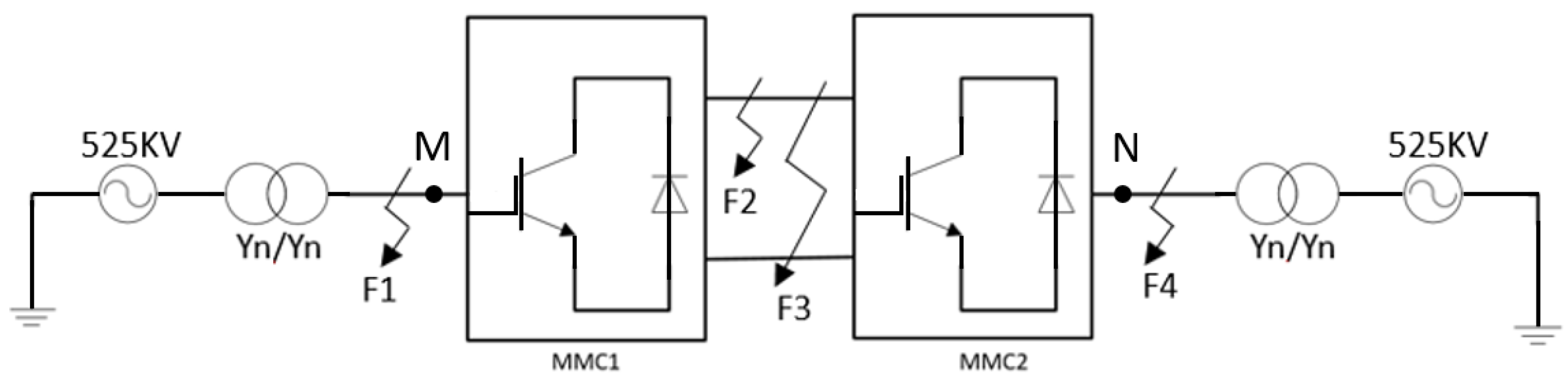
Energies 11 01534 g001
Figure 2. Back-to-back (BTB) modular multilevel converter-based high-voltage direct current (MMC-HVDC) model.
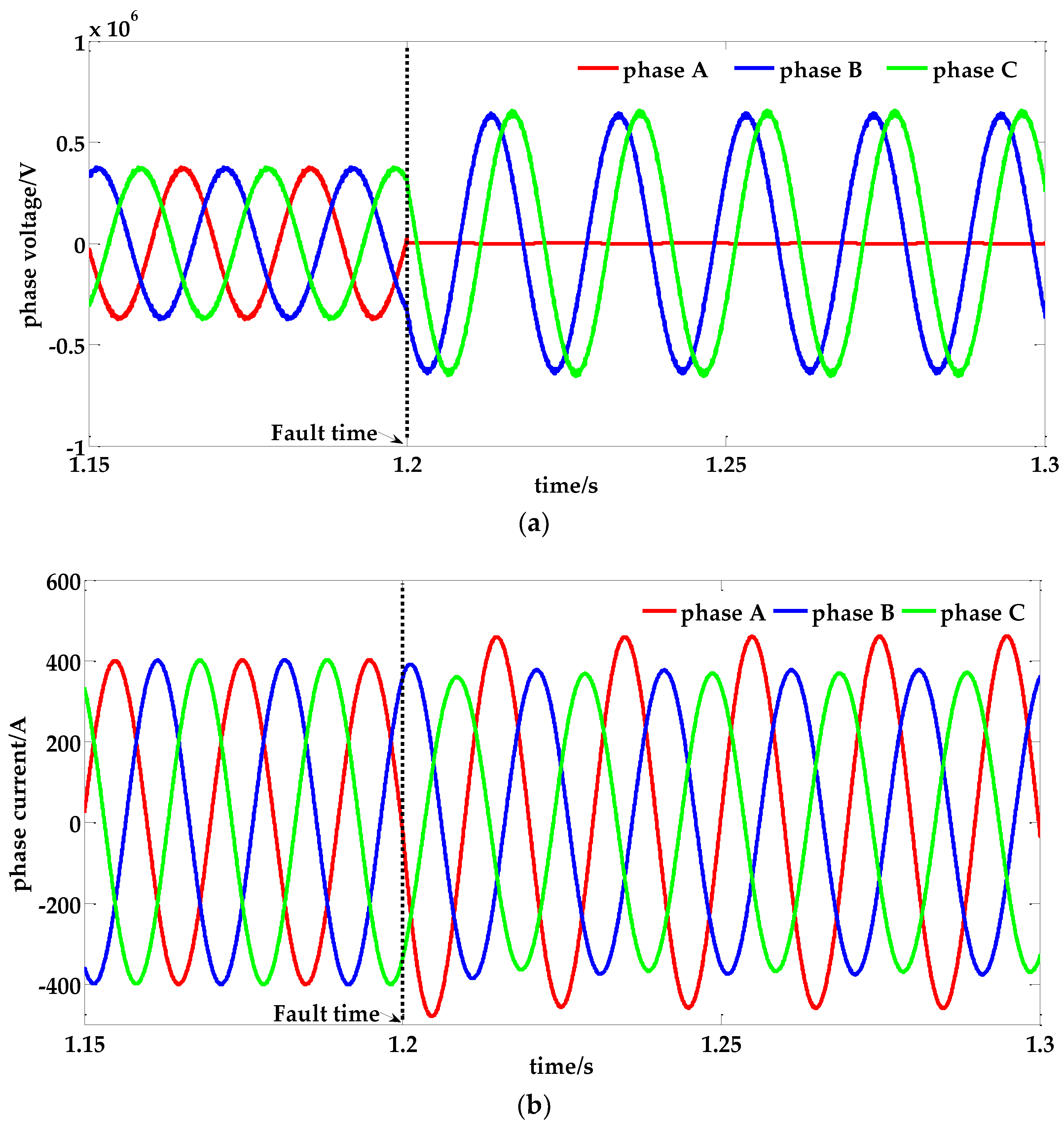
Energies 11 01534 g002
Figure 3. Fault transients under a single-phase grounded fault at the rectifier side. (a) Phase voltage; (b) Phase current.
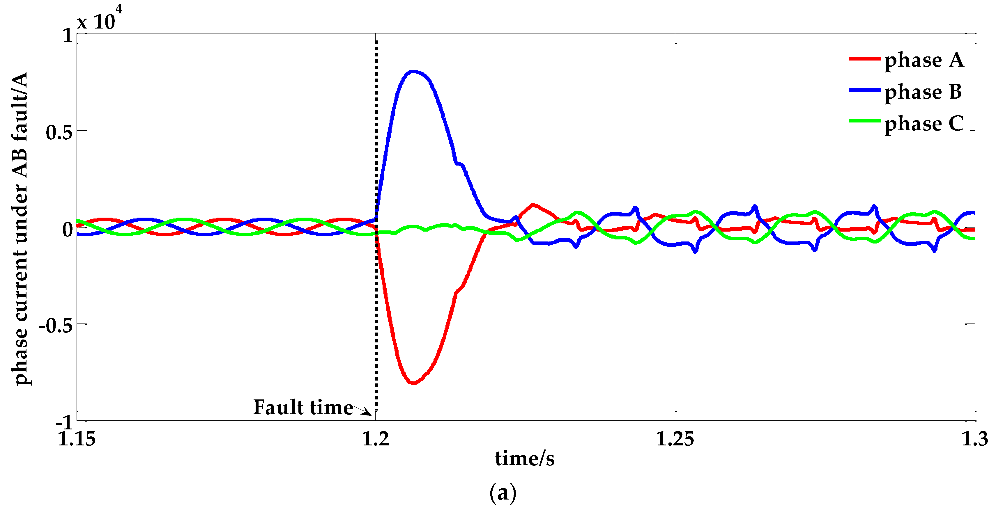
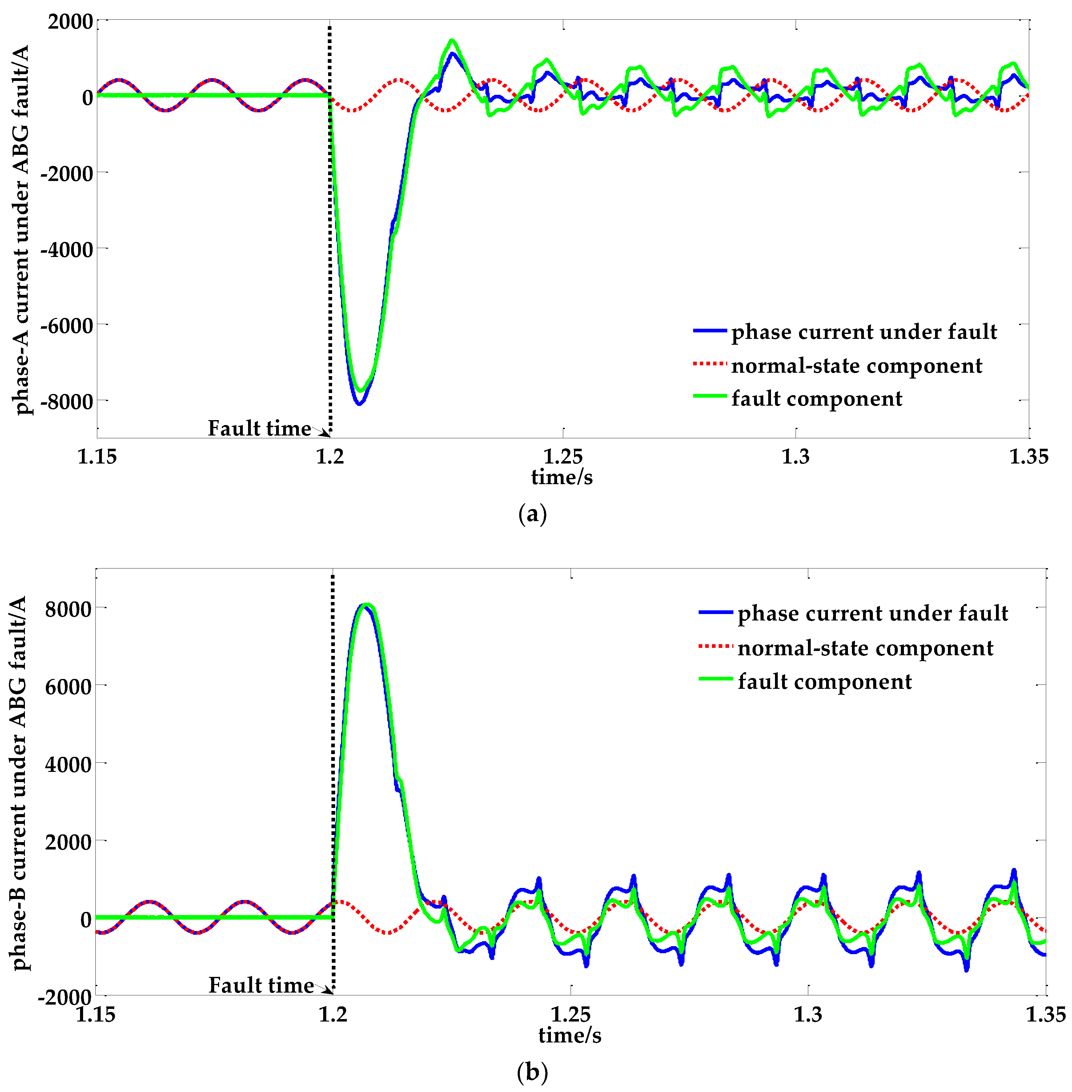
Energies 11 01534 g003
Figure 4. Fault current at point M under (a) AB-phase ungrounded (AB) short-circuit fault; (b) AB-phase grounded (ABG) short-circuit fault.
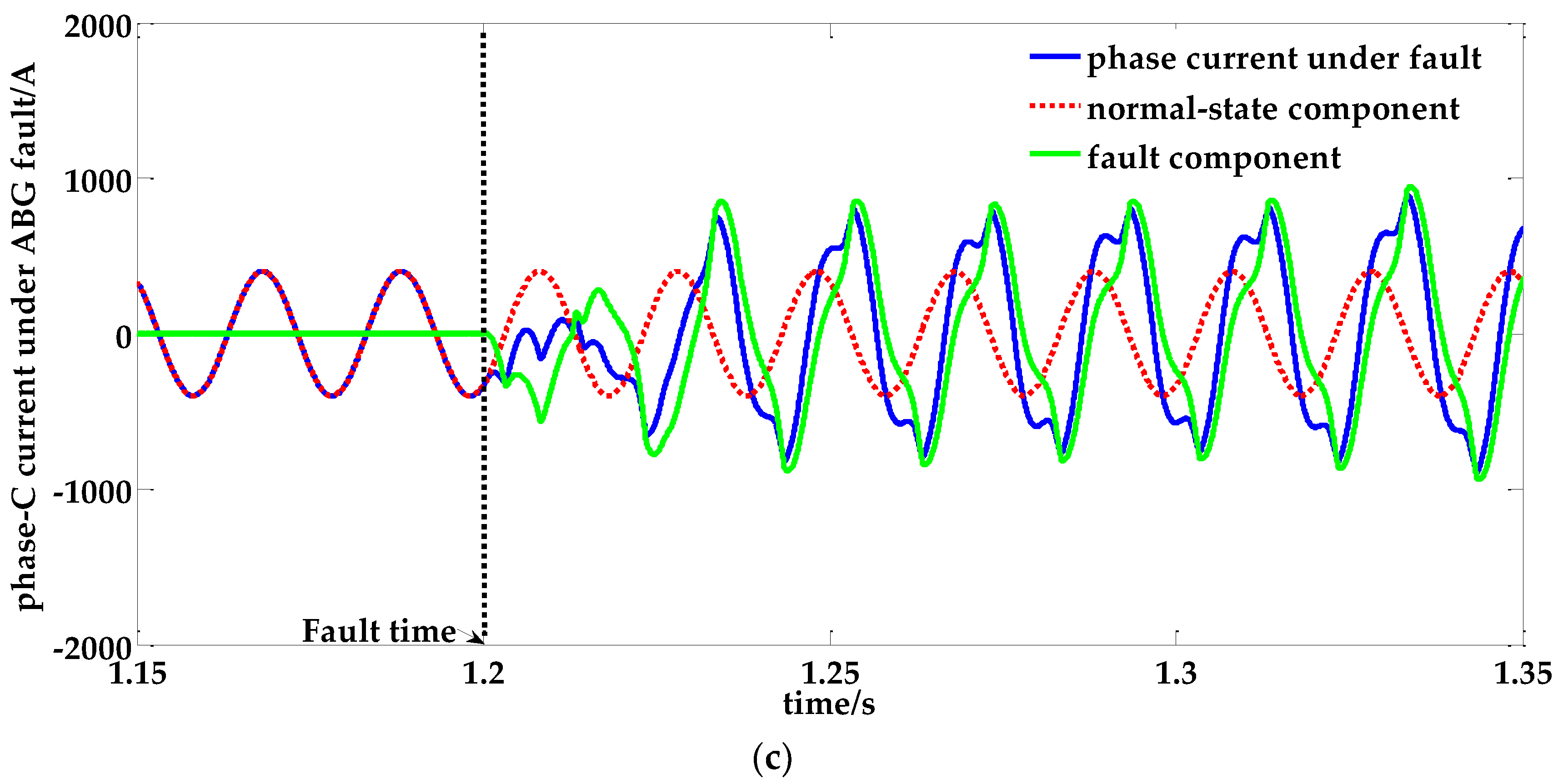
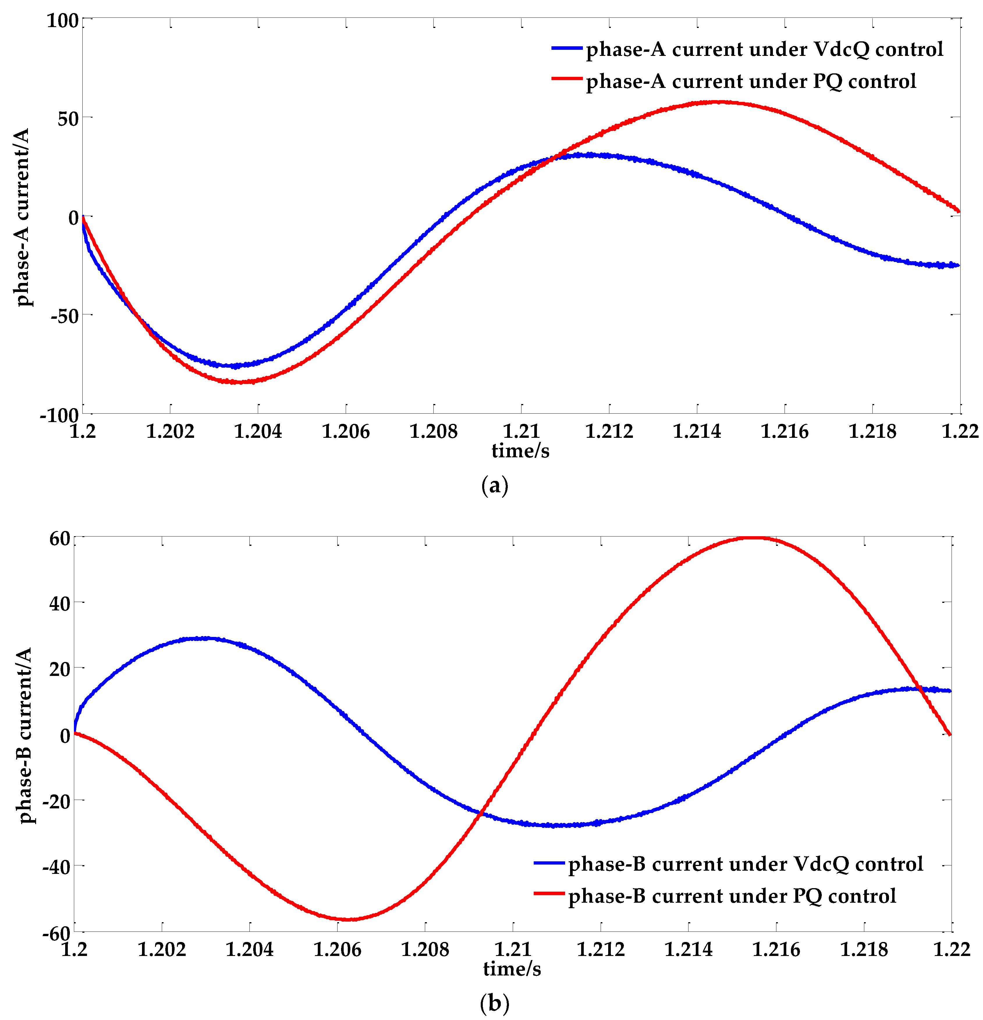
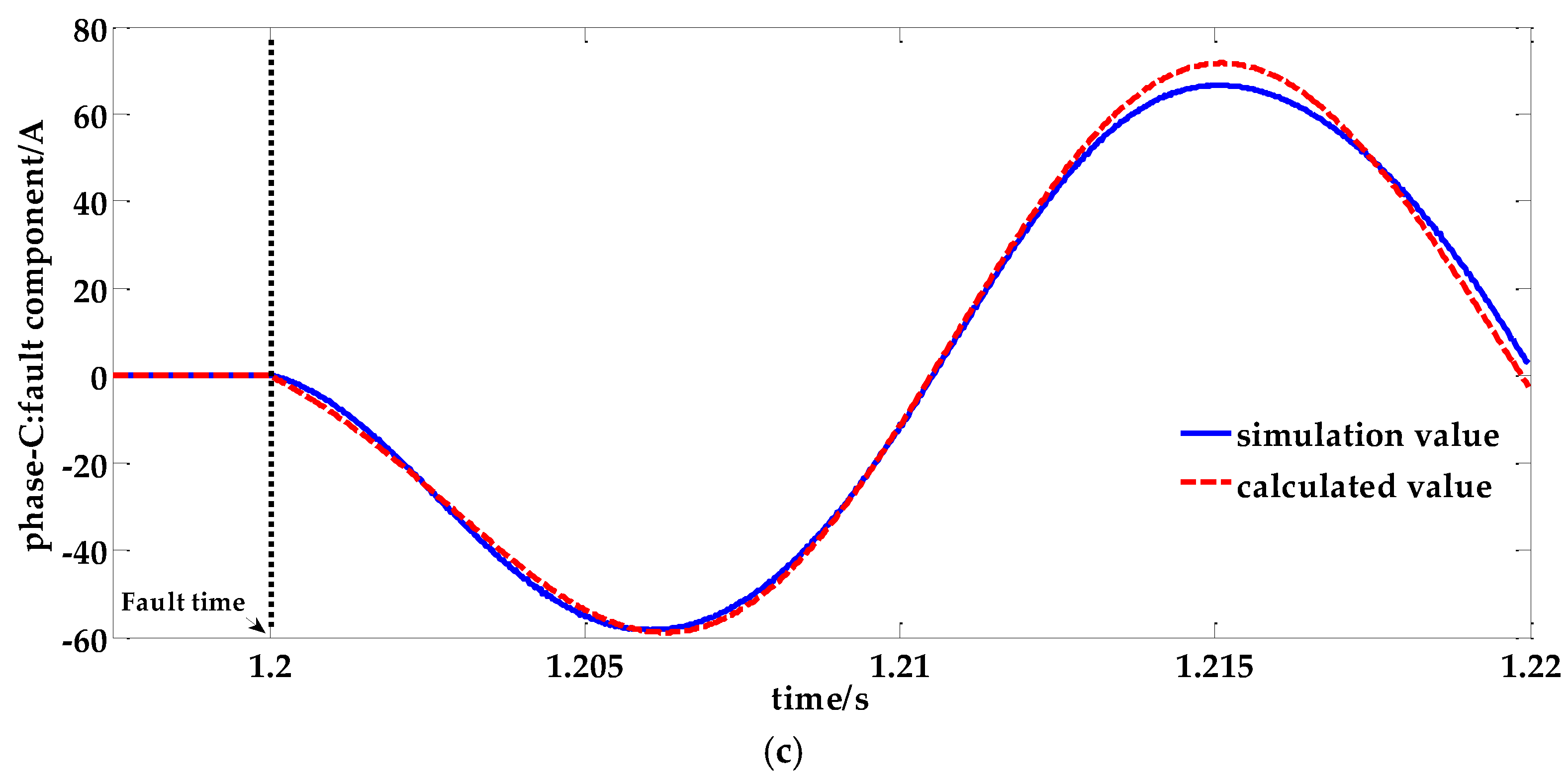
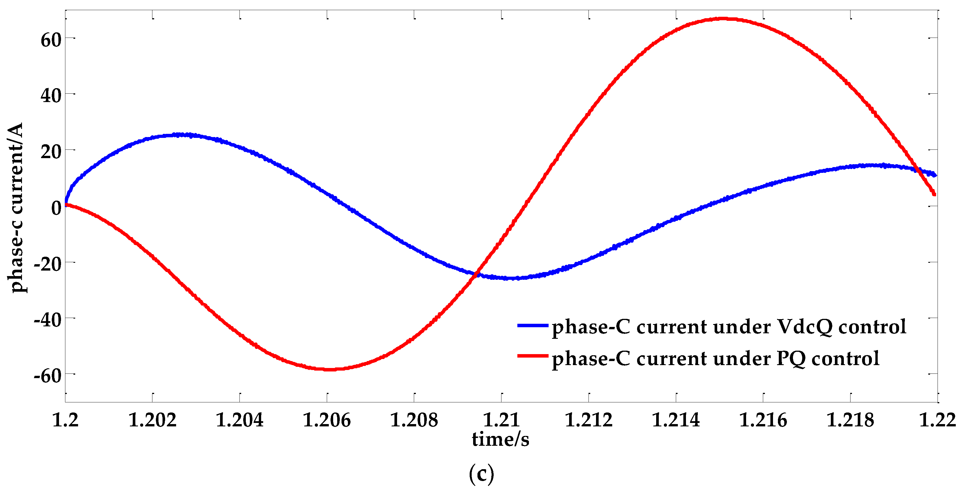
Energies 11 01534 g004aEnergies 11 01534 g004b
Figure 5. Fault component of the phase current under the ABG fault: (a) phase-A current; (b) phase-B current; (c) phase-C current.
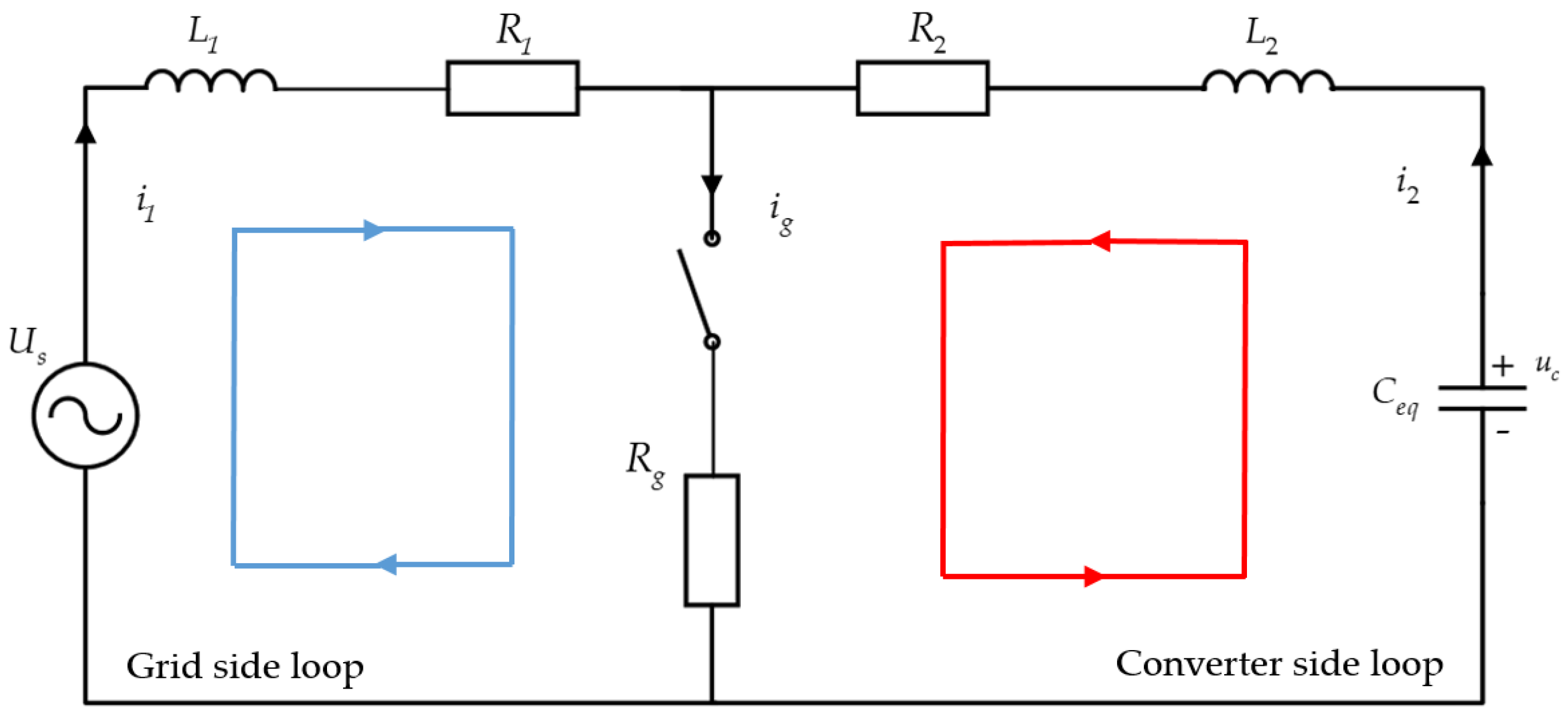
Energies 11 01534 g005aEnergies 11 01534 g005b
Figure 6. Equivalent circuit of a single-phase grounded short-circuit fault.
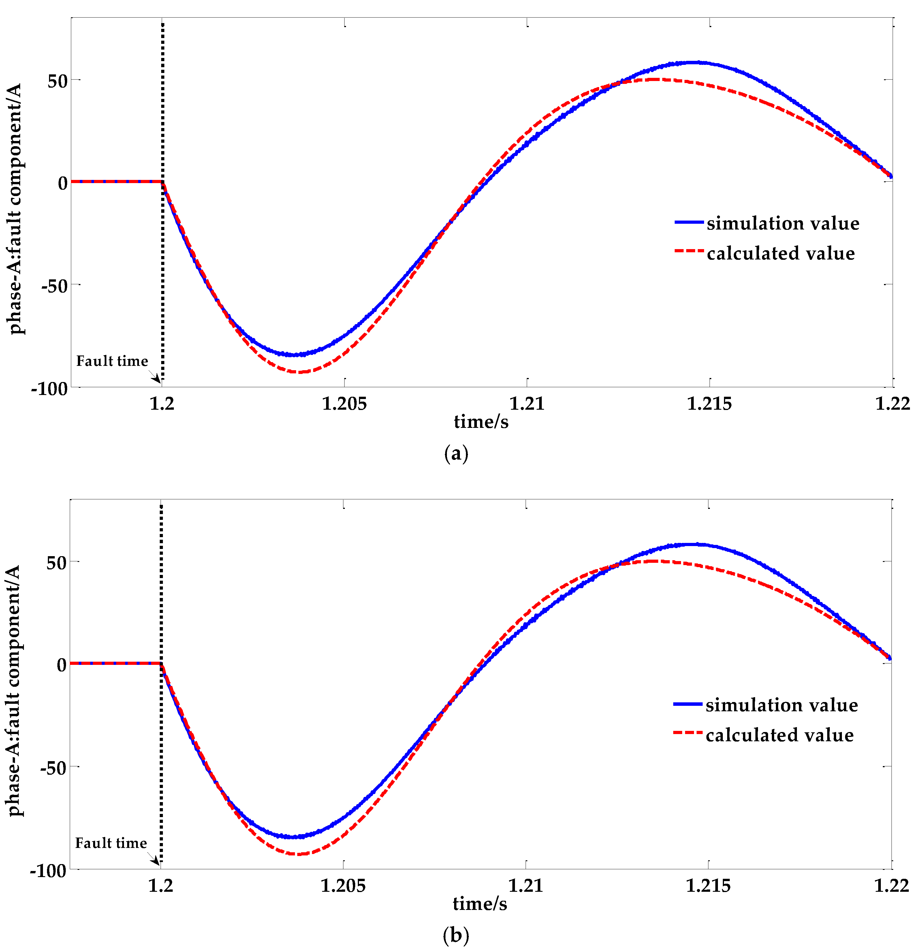
Energies 11 01534 g006
Figure 7. Simulation and calculated values of the three phase currents under phase-A grounded (AG) fault: (a) phase-A current; (b) phase-B current; (c) phase-C current.
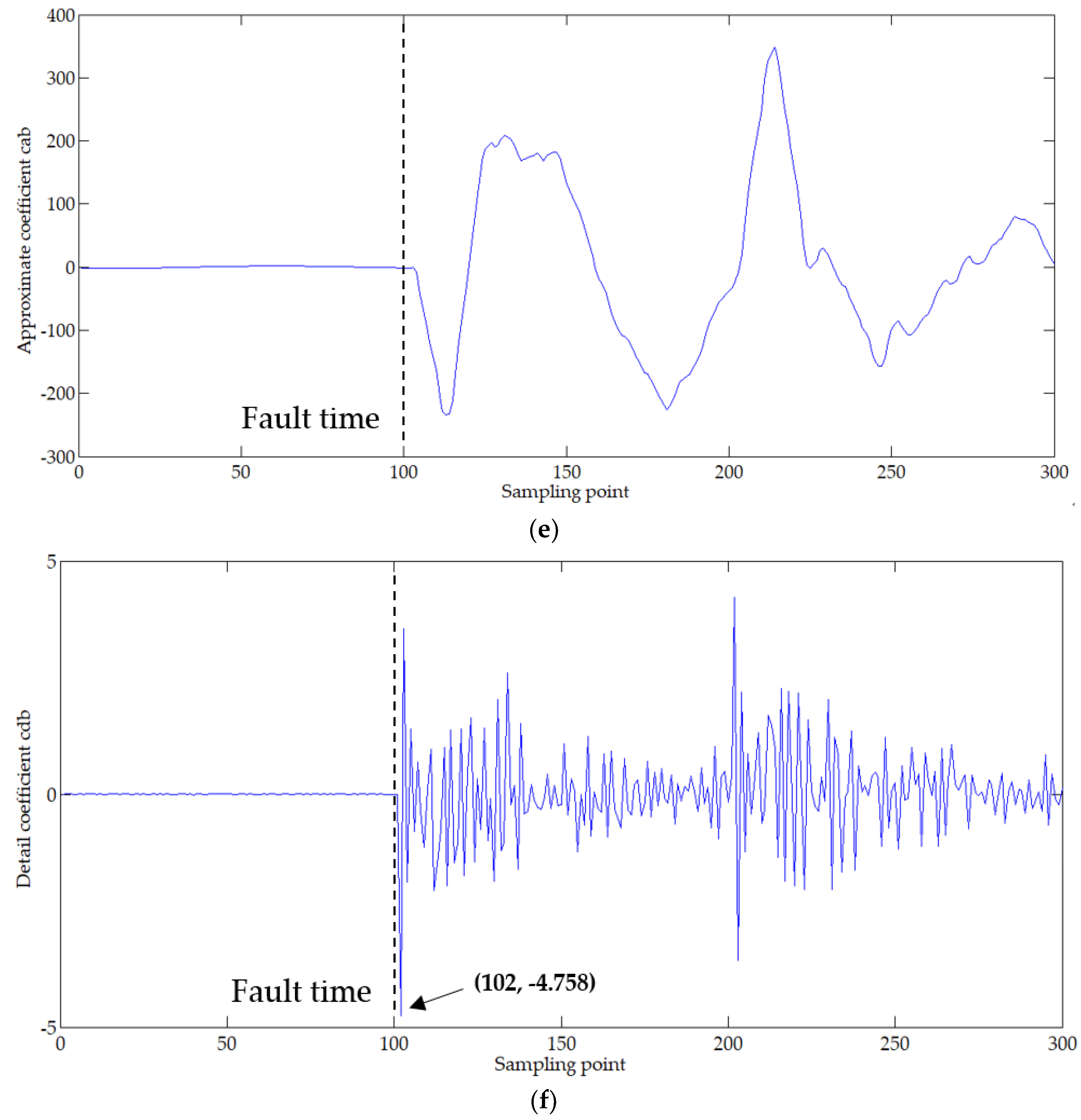
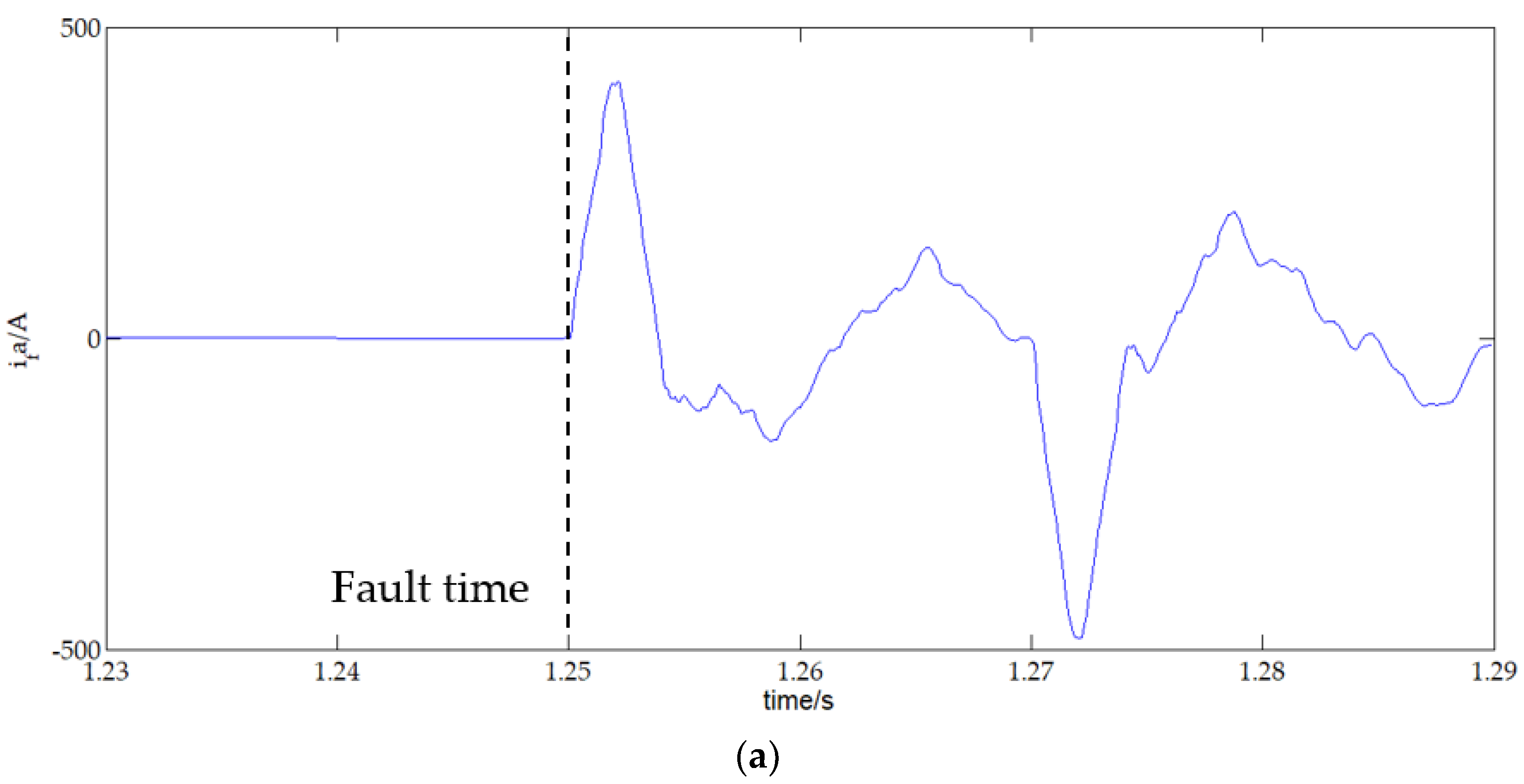
Energies 11 01534 g007aEnergies 11 01534 g007b
Figure 8. AG fault and sound phase current signals under wavelet transform. Phase-A: (a) original phase current signal; (b) approximate coefficient; (c) detail coefficient; phase-B: (d) original phase current signal; (e) approximate coefficient; (f) detail coefficient.
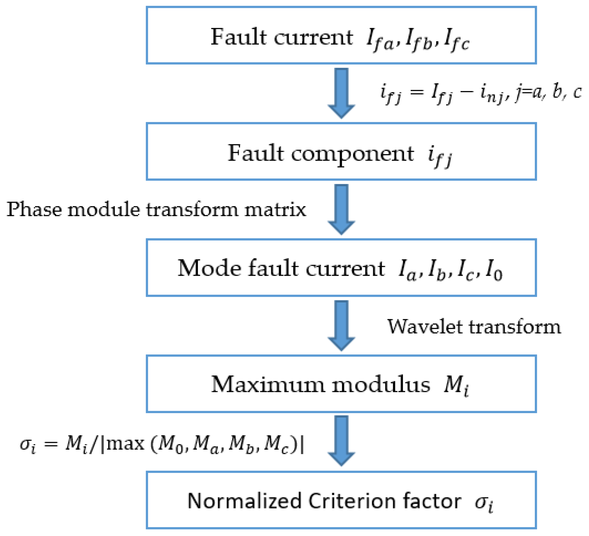
Energies 11 01534 g008aEnergies 11 01534 g008bEnergies 11 01534 g008c
Figure 9. Flowchart for processing fault current signal.
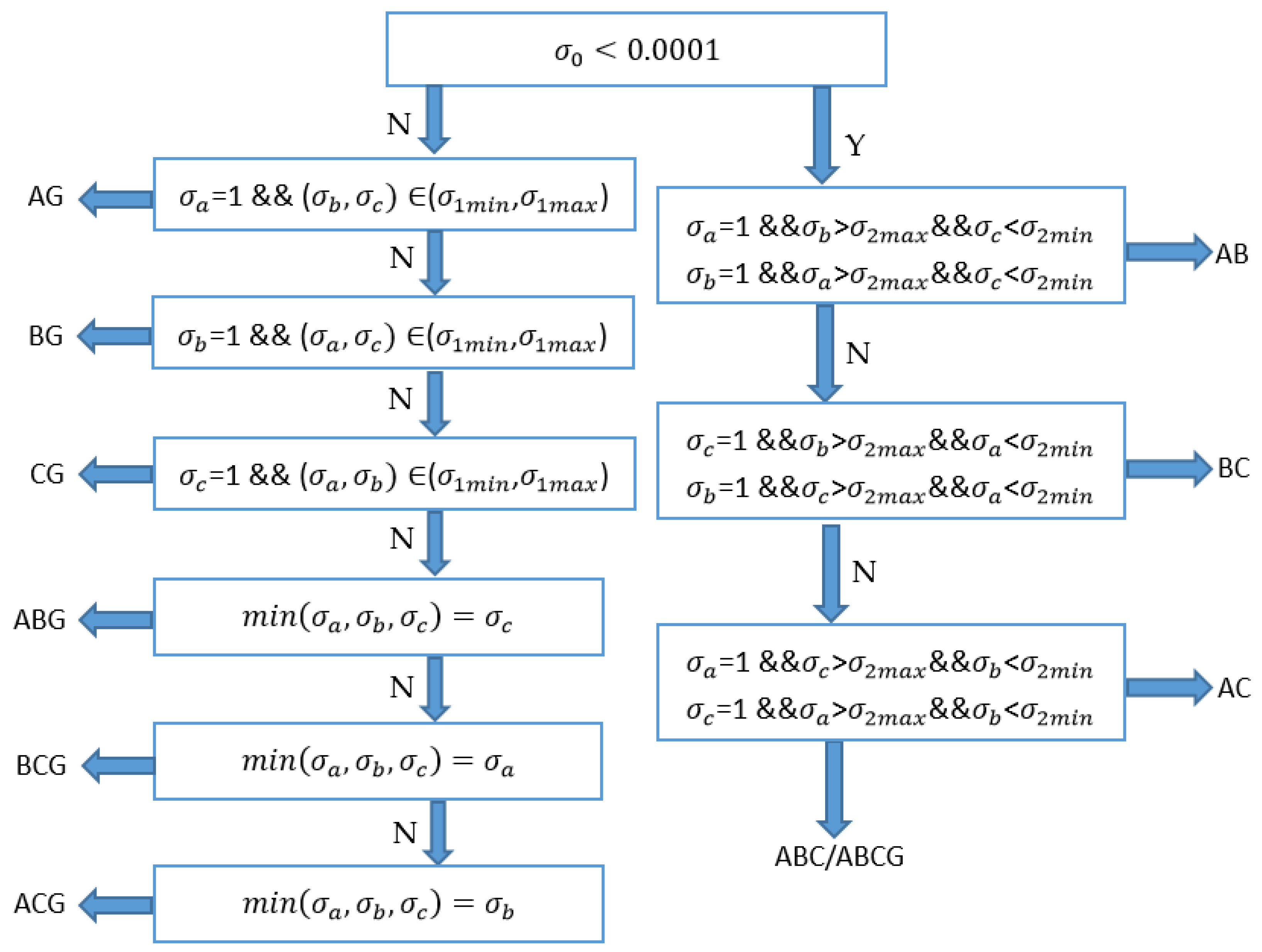
Energies 11 01534 g009
Figure 10. Fault classification scheme.
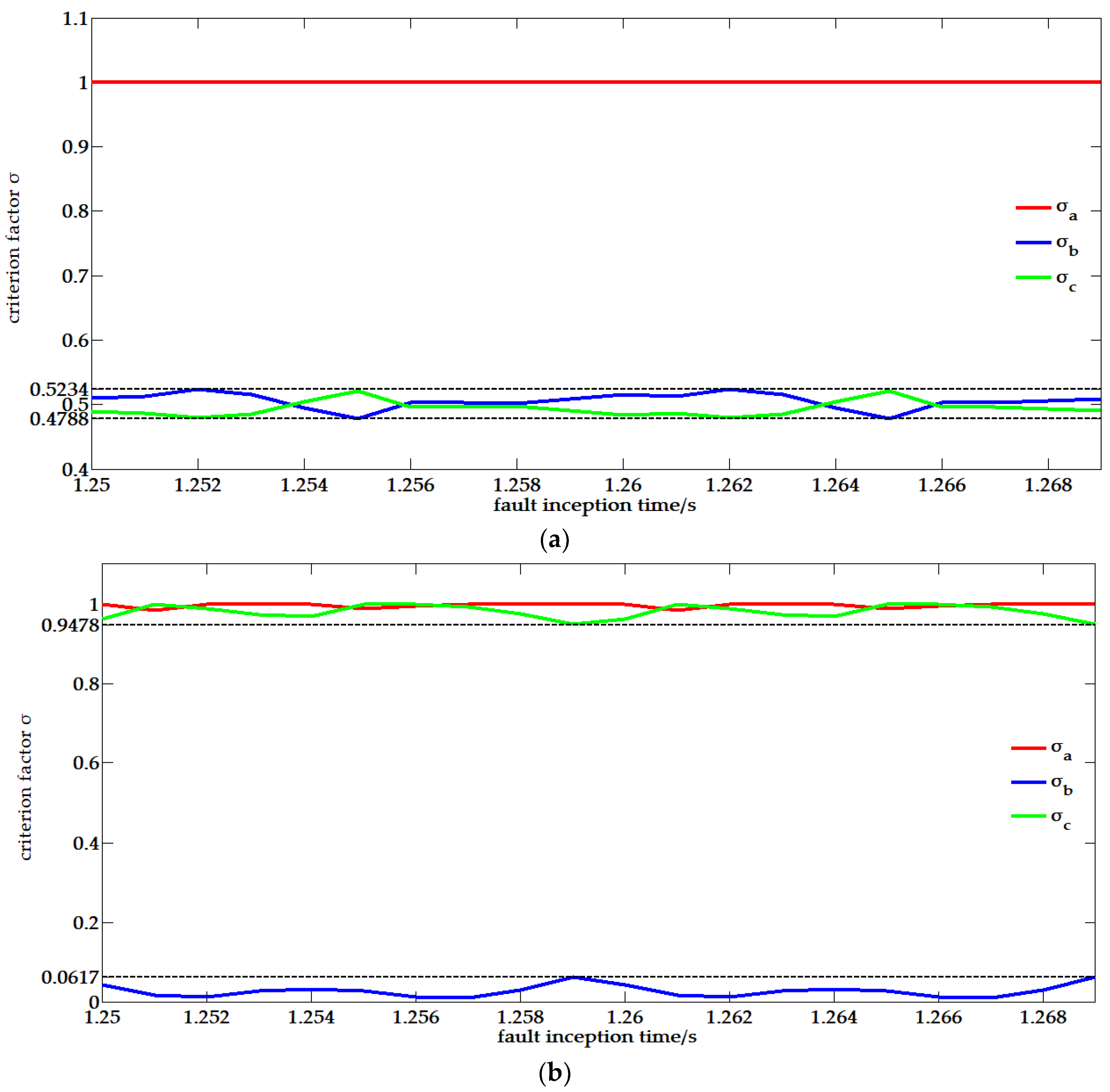
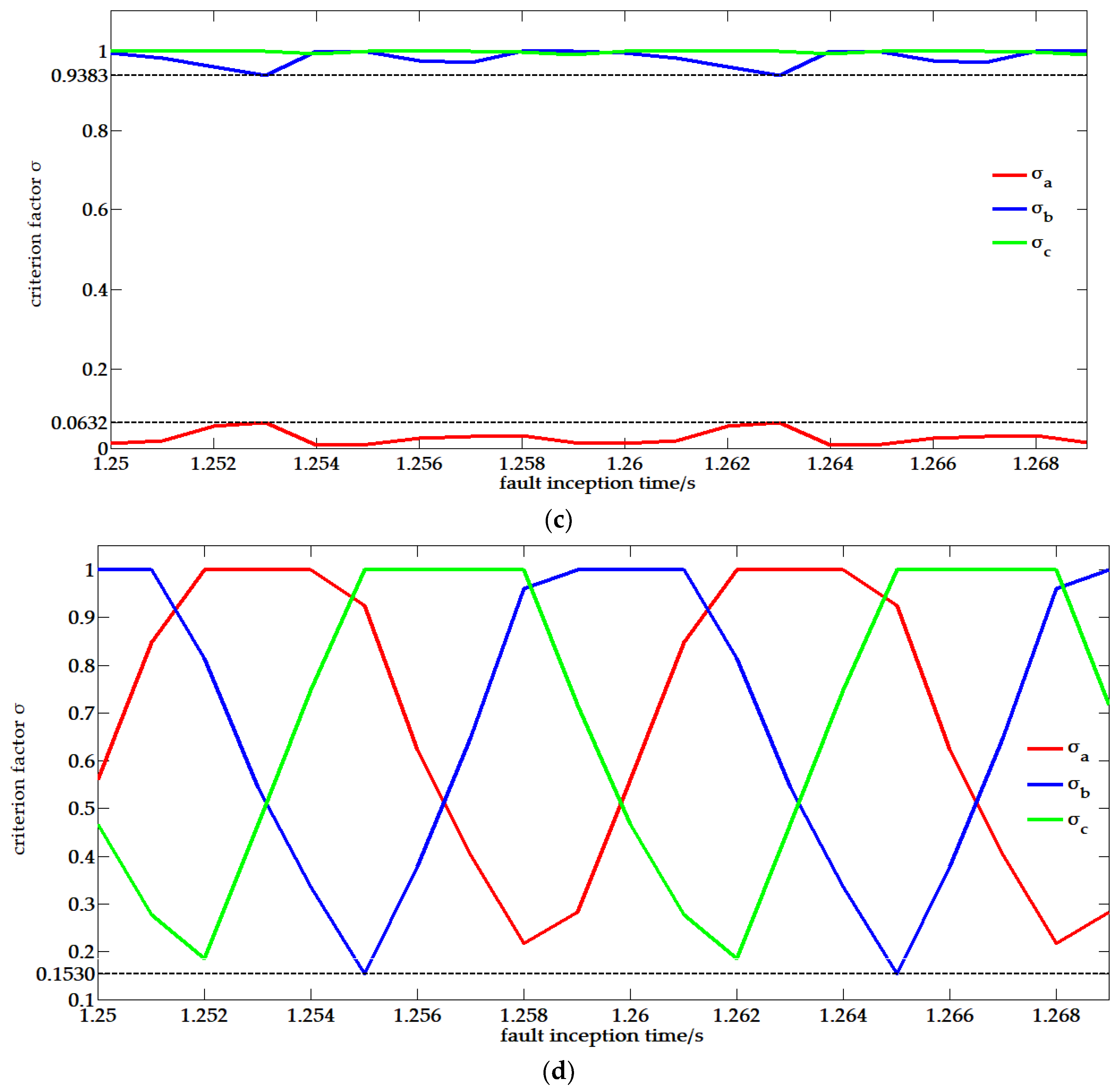
Energies 11 01534 g010
Figure 11. Criterion factors of the different fault types with variable fault inception time of the whole cycle: (a) AG; (b) ACG; (c) BC; (d) ABC.
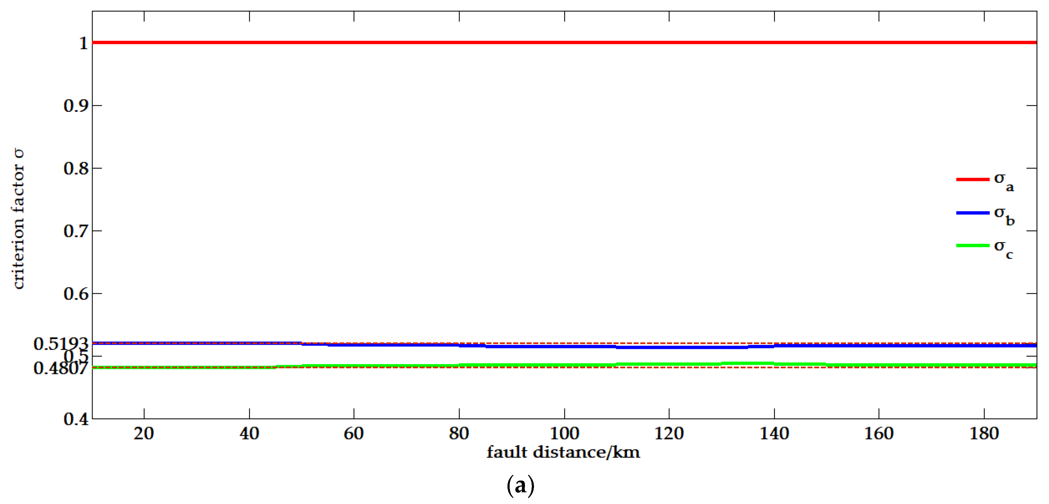
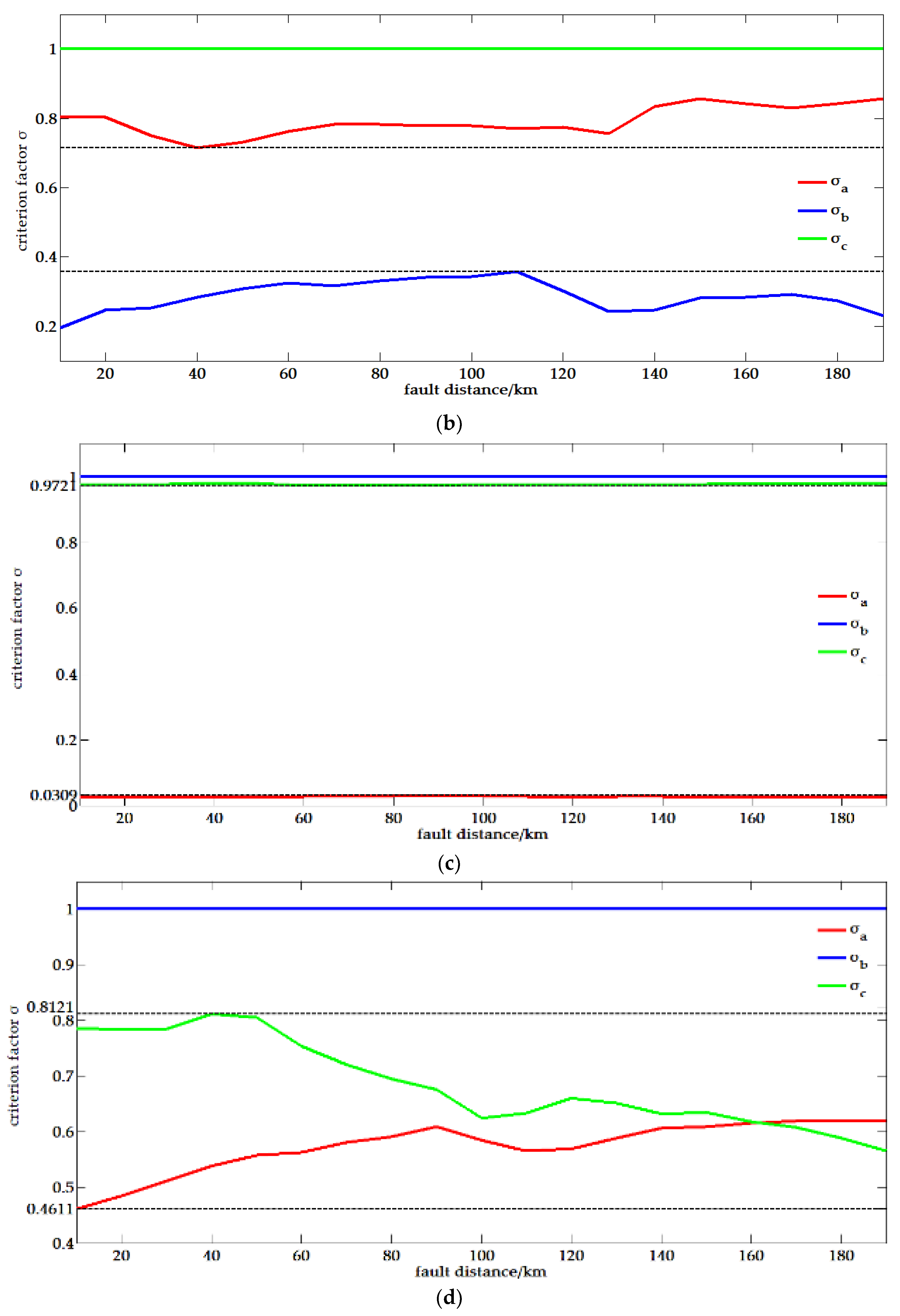
Energies 11 01534 g011aEnergies 11 01534 g011b
Figure 12. Criterion factors of different fault types with variable fault distance from the bus, (a) AG; (b) ACG; (c) BC; (d) ABC.
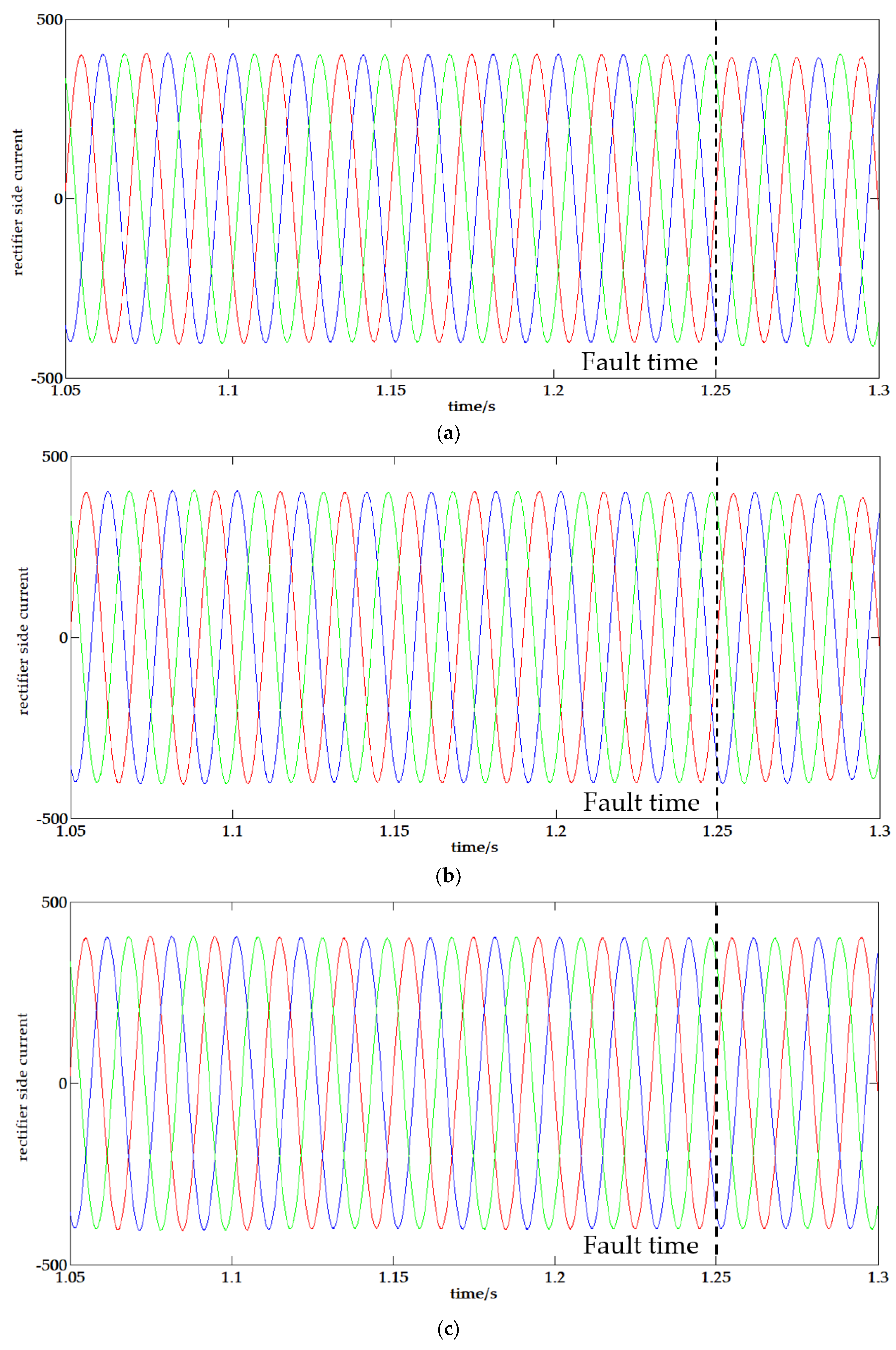
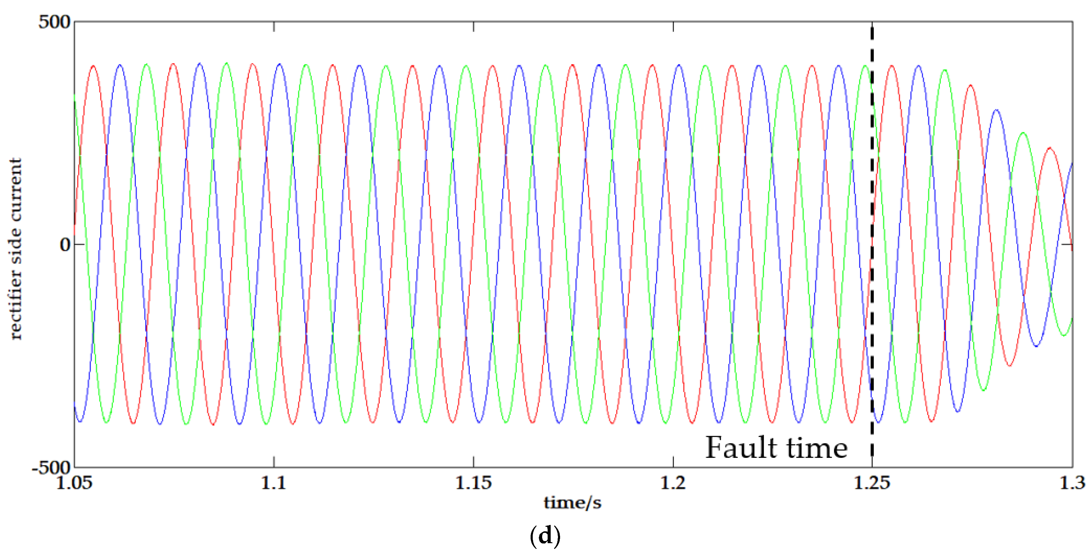
Energies 11 01534 g012aEnergies 11 01534 g012b
Figure 13. Rectifier-side current under inverter-side faults: (a) AG; (b) ACG; (c) BC; (d) ABC. (Red line-phase A; Blue line-phase B; Green line-phase C).
Energies 11 01534 g013aEnergies 11 01534 g013b
Figure 14. Phase current measured at point M under phase-A grounded fault: (a) phase-A; (b) phase-B; (c) phase-C.
Energies 11 01534 g014aEnergies 11 01534 g014b
Table 1. BTB MMC-HVDC system parameters.
System Parameters
DC voltage±420 kVSubmodule number60
Rated power1250 MWBridge inductance140 mH
Short-circuit ratio20Internal groundingYg
AC voltage450 kVAC line length200 km
Frequency50 HzLine resistance12.73 m Ω / km
Transformer voltage525 kV/450 kVLine inductance0.9937 mH
Transformer groundingYn/ynLine capacitance12.74 nF/km
Magnetization resistance99,866 Ω Magnetization inductance321.09 H
Winding resistance1.498 Ω Leakage inductance0.096326 H
Table 2. Characteristics of the mode fault current modulus.
Fault TypeCharacteristics of the Mode Fault Current
IaIbIcI0
AG 2 i a i a i a ≠0
BG i b 2 i b i b ≠0
CG i c i c 2 i c ≠0
ABG 2 i a i b 2 i b i a i a i b ≠0
ACG 2 i a i c i a i c 2 i c i a ≠0
BCG i b i c 2 i b i c 2 i c i b ≠0
AB 3 i a 3 i a 00
AC 3 i c 0 3 i c 0
BC0 3 i b 3 i b 0
ABCG 2 i a i b i c 2 i b i a i c 2 i c i a i b 0
ABC 3 i a 3 i b 3 i c 0
Table 3. Criterion factor of the calculated current of the different fault types (resistance R = 0.001 Ω, fault distance d = 100 km, fault inception time: A phase voltage cross zero [1.200 s]).
Fault TypeWindow Length σ a σ b σ c σ 0
AG1 ms10.50680.49320.0474
2 ms10.50850.49140.0795
3 ms10.50860.49140.1579
4 ms10.50860.49140.1879
5 ms10.50860.49140.1998
ABG1 ms0.786110.21390.0234
2 ms10.95110.17130.0142
3 ms0.999410.12260.0101
4 ms0.960110.09280.0077
5 ms0.953610.07890.0065
AC1 ms10.03340.98620
2 ms10.03620.96870
3 ms10.03620.96870
4 ms0.98030.025410
5 ms10.03410.96590
ABC1 ms0.222610.77740
2 ms0.399210.60080
3 ms0.592210.47180
4 ms0.781410.41630
5 ms0.982010.39980
Table 4. Criterion factor of the simulation current of the different fault types (resistance R = 0.001 Ω, fault distance d = 100 km, fault inception time: A phase voltage cross zero [1.200 s]).
Fault Type σ a σ b σ c σ 0
AG10.51030.48970.0732
BG0.485610.51440.0735
CG0.49570.504310.0774
ABG0.901710.10920.0142
ACG0.74700.282610.0433
BCG0.046410.95360.0037
AB0.985810.01420
AC10.03920.96430
BC0.018610.98140
ABCG0.257110.74290
ABC0.257110.74290
Table 5. Criterion factor of the different fault types with variable fault inception angle (resistance R = 0.001 Ω, fault distance d = 180 km from the bus).
Fault TypeFault Inception Angle σ a σ b σ c σ 0 Fault Classification Result
AG1/5π10.52350.48010.0947AG
AG2/5π10.49530.50470.0812AG
AG1/2π10.47880.52120.0780AG
ACG1/5π10.01210.98790.0021ACG
ACG2/5π10.03190.96810.0041ACG
ACG1/2π0.98710.026410.0118ACG
BC1/5π0.05610.959410BC
BC2/5π0.007310.99270BC
BC1/2π0.00910.997010BC
ABC1/5π10.81520.18480ABC
ABC2/5π10.33480.74850ABC
ABC1/2π0.92450.153010ABC
Table 6. Criterion factor of different fault types with variable fault distance from the bus (resistance R = 100 Ω, fault inception time: A phase voltage cross zero [1.250 s]).
Fault TypeFault Distance σ a σ b σ c σ 0 Fault Classification Result
AG20 km10.51900.48100.1446AG
AG100 km10.51290.48840.1216AG
AG180 km10.51590.48410.1016AG
ACG20 km0.80290.246710.0530ACG
ACG100 km0.77950.342910.0487ACG
ACG180 km0.84210.272710.0430ACG
BC20 km0.026210.97410BC
BC100 km0.029610.97620BC
BC180 km0.025310.97900BC
ABC20 km0.483710.78390ABC
ABC100 km0.584810.62440ABC
ABC180 km0.619110.58760ABC
Table 7. Criterion factor of the different fault types with variable resistance (fault distance d = 180 km from the bus, fault inception time: A phase voltage cross zero [1.250 s]).
Fault TypeFault Resistance σ a σ b σ c σ 0 Fault Classification Result
AG0.00110.51570.48430.0999AG
AG10010.51590.48410.1016AG
AG50010.51930.48080.1025AG
ACG0.00110.04200.96240.0542ACG
ACG1000.84210.272710.0430ACG
ACG5000.94510.107310.0222ACG
BC0.0010.01130.995210BC
BC1000.025310.97900BC
BC5000.016810.99170BC
ABC0.0010.560610.46750ABC
ABC1000.619110.58760ABC
ABC5000.484610.61270ABC
Table 8. Criterion factor of DC faults F2 and F3 with variable fault inception time (resistance R = 0.001 Ω, F2+ means a positive pole-to-ground fault, F2− denotes a negative pole-to-ground fault).
Fault TypeFault Inception Angle σ a σ b σ c σ 0
F2+00.00070.00230.00211
F2+1/5π0.00170.00250.00121
F2+2/5π0.00250.00180.00091
F2-00.00100.00230.00211
F2−1/5π0.00170.00250.00091
F2−2/5π0.00250.00180.00101
F300.922810.15260
F31/5π10.46320.53680
F32/5π0.84720.152810
Table 9. Criterion factor of the inverter-side faults.
Fault Type σ a σ b σ c σ 0
AG0.02120.04650.06761
ACG0.01550.03400.04941
BC0.31450.686910.0898
ABC0.31450.686910.1087
Normal0.31630.684810.0033
Table 10. Contrast test under V d c Q control mode (resistance R = 0.001 Ω, fault distance d = 100 km, fault inception time: A phase voltage cross zero [1.200 s]).
Fault Type σ a σ b σ c σ 0
AG10.51820.48180.0609
BG0.496710.50340.0628
CG0.49800.502010.0548
ABG0.987910.01210.0011
ACG0.97040.043410.0050
BCG0.010010.99000.0004
AB0.995910.00410
AC10.01590.98940
BC0.006310.99370
ABCG0.285710.71430
ABC0.257110.74290
Table 11. Test result with different power load: (a) P = 0.1 p.u. Q = 0; (b) P = 0.25 p.u. Q = 0; (c) P = 0.2 p.u. Q = 0.1 (resistance R = 0.001 Ω, fault distance d = 100 km, fault inception time: A phase voltage cross zero [1.200 s]).
(a)
Fault Type σ a σ b σ c σ 0
AG10.48990.51010.7317
BG0.500110.49990.8036
CG0.50050.499510.7270
ABG0.985710.01430.0124
ACG10.01770.98230.0279
BCG0.013010.98700.0027
AB0.993810.00620
AC10.03490.96510
BC0.011110.98890
ABCG0.213710.78630
ABC0.213710.78630
(b)
Fault Type σ a σ b σ c σ 0
AG10.49710.50290.7376
BG0.506510.49390.7936
CG0.49400.506010.7292
ABG0.985510.01450.0111
ACG10.02130.98840.0365
BCG0.015410.98460.0033
AB0.992610.00740
AC10.03310.96690
BC0.013110.98690
ABCG0.211310.78870
ABC0.211310.78870
(c)
Fault Type σ a σ b σ c σ 0
AG10.50120.49880.7347
BG0.499610.50040.7931
CG0.49290.507110.7216
ABG0.984810.01520.0115
ACG10.01890.98910.0333
BCG0.013310.98670.0030
AB0.992310.00770
AC10.03060.96940
BC0.011210.98880
ABCG0.229610.77040
ABC0.229610.77040
Table 12. Detection time comparison of fault diagnosis methods.
Fault Diagnosis MethodMain TechniqueDetection Time
Reference 9Phase current difference20 ms
Reference 10Change rate of phase current phasor5 ms
Reference 11Time-frequency characteristics of transient travelling wave2.5 ms
Reference 12Artificial immune algorithm & transient current energy5 ms
Reference 14Renyi wavelet packet time entropy20 ms
This paperDWT & Modulus maxima1 ms

