Static and Dynamic Networking of Smart Meters Based on the Characteristics of the Electricity Usage Information

Abstract

The normal communication between smart meter and concentrator is a key factor influencing the normal function of users’ power consumption systems. To solve the communication failure of the smart meter caused by the signal conflict as well as the collected consecutive information abnormality from the same smart meter, according to the chain optimization index, the networking method of static and dynamic combination proposed in this paper is first used to picked out the optimal relay for a smart meter belonging to multiple relay communication ranges. Meanwhile, the communication with other secondary relays is closed to avoid signal conflict. Then the paper forms different combinations of collected data and these combinations are trained in the extreme learning machine (ELM) to find the characteristics value of power consumption information. Finally, in MATLAB simulation, if ELM detects the abnormal information, new communication path could be promptly found through dynamic adjustment of chain optimization weighted coefficient and the weighted coefficient of the number of the relayed smart meters. It solves the problem of consecutive information abnormality from the same smart meter and raises the reliability of smart meter’s communication, having a significantly meaning to guarantee the normal function of users’ power consumption system.

1. Introduction

With the large-scale use of smart meters, electricity information acquisition systems have become the largest automatic electric energy measurement system. The accurate collection of smart meter information not only affects the normal work of the power user electric energy data acquisition system, but also helps empower utility companies and users to make more informed energy management decisions, and examples such as the success of the demand response program in [1], the analysis of the customers’ willingness to participate in load management programs in [2], and the informed energy management decisions in [3,4] all rely on the accurate collection of electricity information from smart meters.

1.1. Motivation

The effective transmission of high quality communication signals with the existing power line architectures is a potential and important means to achieve energy and information circulation between the energy and the Internet in the future [5,6,7]. However, because the power line channel has the characteristics of noise interference, impedance input, multipath effect, signal attenuation and so on [8,9,10,11], the transmission distance of data signals will change with the quality of the channels in the network. Therefore, in order to increase the transmission distance of data signals, networking technology is used in smart meter communication, but in experiments, it found that there are two problems in smart meter networking: one is the communication failure due to signal conflict, which is caused by multiple relays communicating with the same smart meter at the same time, and the other is the abnormality of information collected from smart meters. If the abnormality of information collected cannot be detected in time, a new communication path will not be established, and as a result, the collected information continues to be abnormal. Our challenge is to overcome these two problems in current smart meter networking.

1.2. Literature Survey

Many artificial intelligence algorithms are widely used in low-voltage power line networking to increase the communication distance. In [12,13,14] artificial cobweb algorithms are used for networking, which can increase the communication distance between the concentrator and smart meters, but will present the signal conflict problem when many relays try to communicate with the smart meter at the same time. References [15,16] adopt an ant colony algorithm for networking and References [17,18] use genetic algorithm for networking, which could find the optimal path for communication, but when the original communication path fails, it cannot dynamically find a new path for communication. Reference [19] uses the idea of a static and dynamic combination to network, which can avoid the signal conflict problem, but when the collected information is abnormal, it cannot find a new path to establish communication in time.

1.3. Contributions

The main contributuins if this work can be summarized as follows:

(1)

The proposed method avoids signal conflicts caused by multiple relays communicating with the same smart meter at the same time.

(2)

When the information collected by the concentrator is abnormal, this paper avoids the situation that the information collected next time is abnormal.

(3)

By means of MATLAB simulation, when a smart meter belongs to the communication range of multiple relays, according to the networking method of static and dynamic combination, the smart meter only communicate with an optimal relay, so it could effectively avoid the signal conflict problem, and when the characteristics of the power information of an smart meter are abnormal, a new communication path could be established in time by dynamically adjusting the link optimization weighting coefficient and the weighting coefficient of the number of relayed and forwarded smart meters, which effectively overcomes the situation of continuous abnormal information coming from a certain smart meter.

1.4. Organization of the Paper

The rest of the paper is organized as follows: Section 2 describes the working principle of the power user electric energy data acquisition system and explains the static and dynamic combination networking method. Section 3 analyzes the characteristics of the collected data, and adjusts the communication path based on whether the eigenvalues are abnormal. Section 4 shows the simulation results using MATLAB. Finally, in Section 5, we give our conclusions.

2. The Power User Electric Energy Data Acquire System and Networking Method

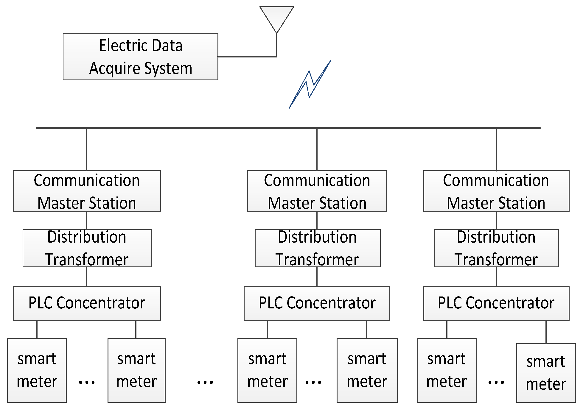
The working principle of the power user electric energy data acquisition system is as follows: in the same transformer power supply range, the concentrator sends a message to smart meters through the low voltage power line, and after receiving the instruction, the smart meters send the data information to the concentrator, the concentrator then sends the electricity information of the smart meters to the communication master station and finally, the master station transmits the data information to the power user electric energy data acquisition system through a special network, as is shown in Figure 1.

In an ideal state, the PLC concentrator can collect the electricity information of all smart meters within the same transformer power supply range. However, in practice, the transmission distance of the signal will be changed due to the noise interference of the power line channel, the multipath effect, the signal attenuation and so on. Therefore, in the same transformer power supply range, in order to increase the communication distance between the concentrator and smart meters, and ensure that the data information of all the smart meters are collected based on low-voltage power line communication, the paper uses the smart meter networking technology to enable the concentrator to communicate with remote smart meters. In the experiments, the transmission distance between the concentrator and the smart meter is 200 to 400 m within the same transformer power supply range, and the transmission distance between the smart meters is about 30 m. Each smart meter not only has the function of sending and receiving the message, but also has a relay function to transmit information to other smart meters. For the limiting conditions of the communication distance between the concentrator and the smart meter, and the static and dynamic combination method used for the smart meter networking, readers may refer to Section 3. The Networking Method of Static and Dynamic Combination

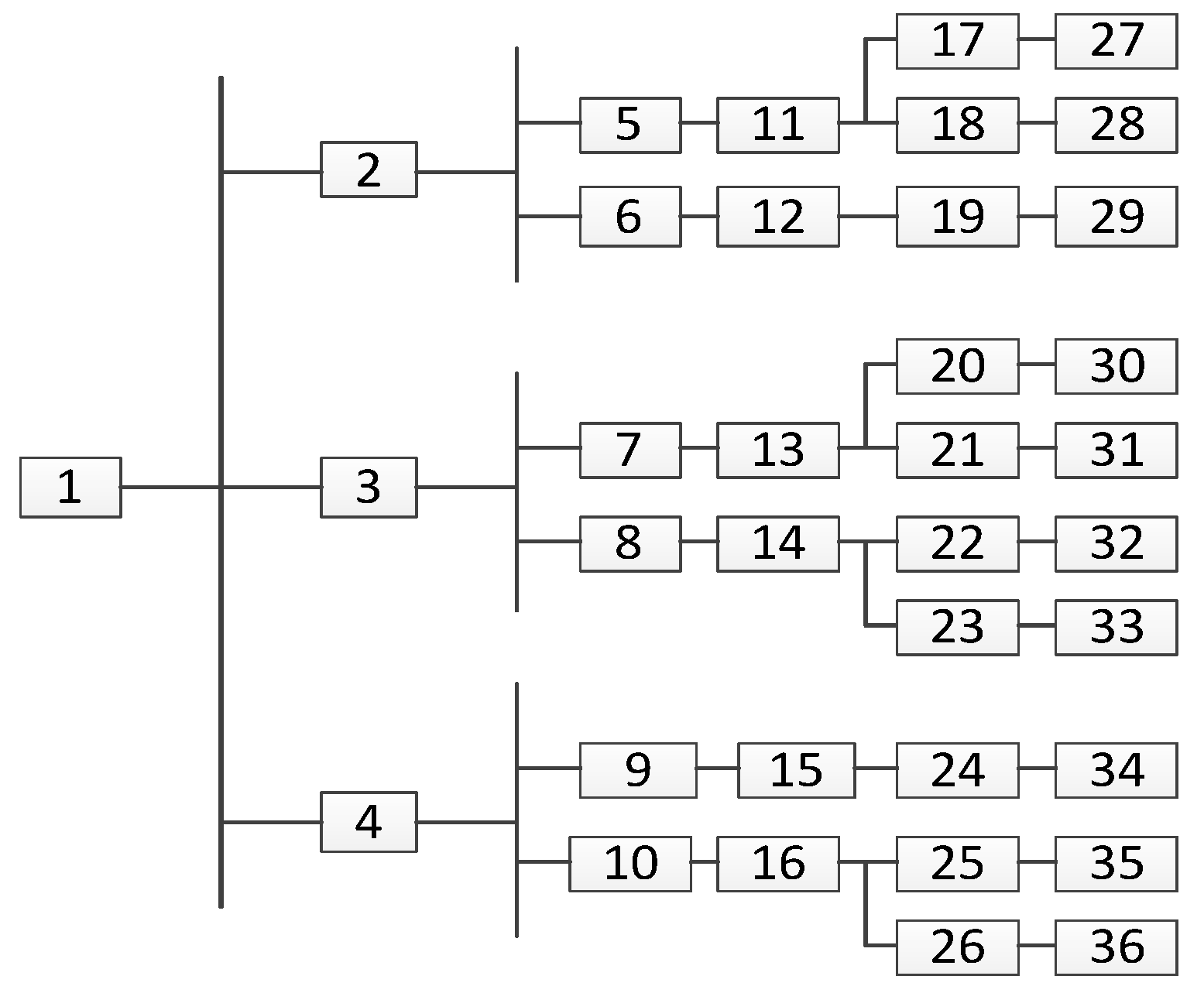
2.1. Network Topology of Smart Meters

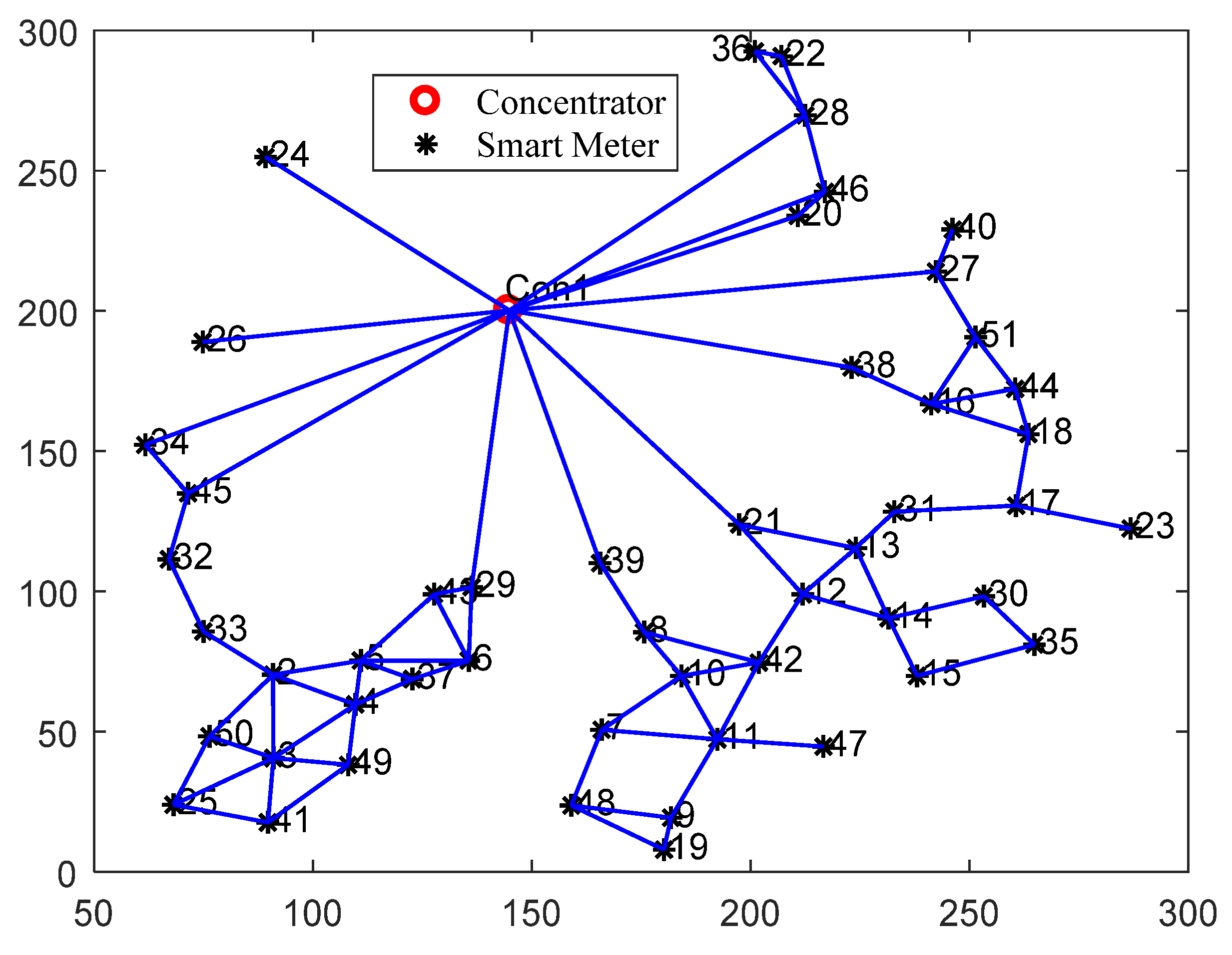
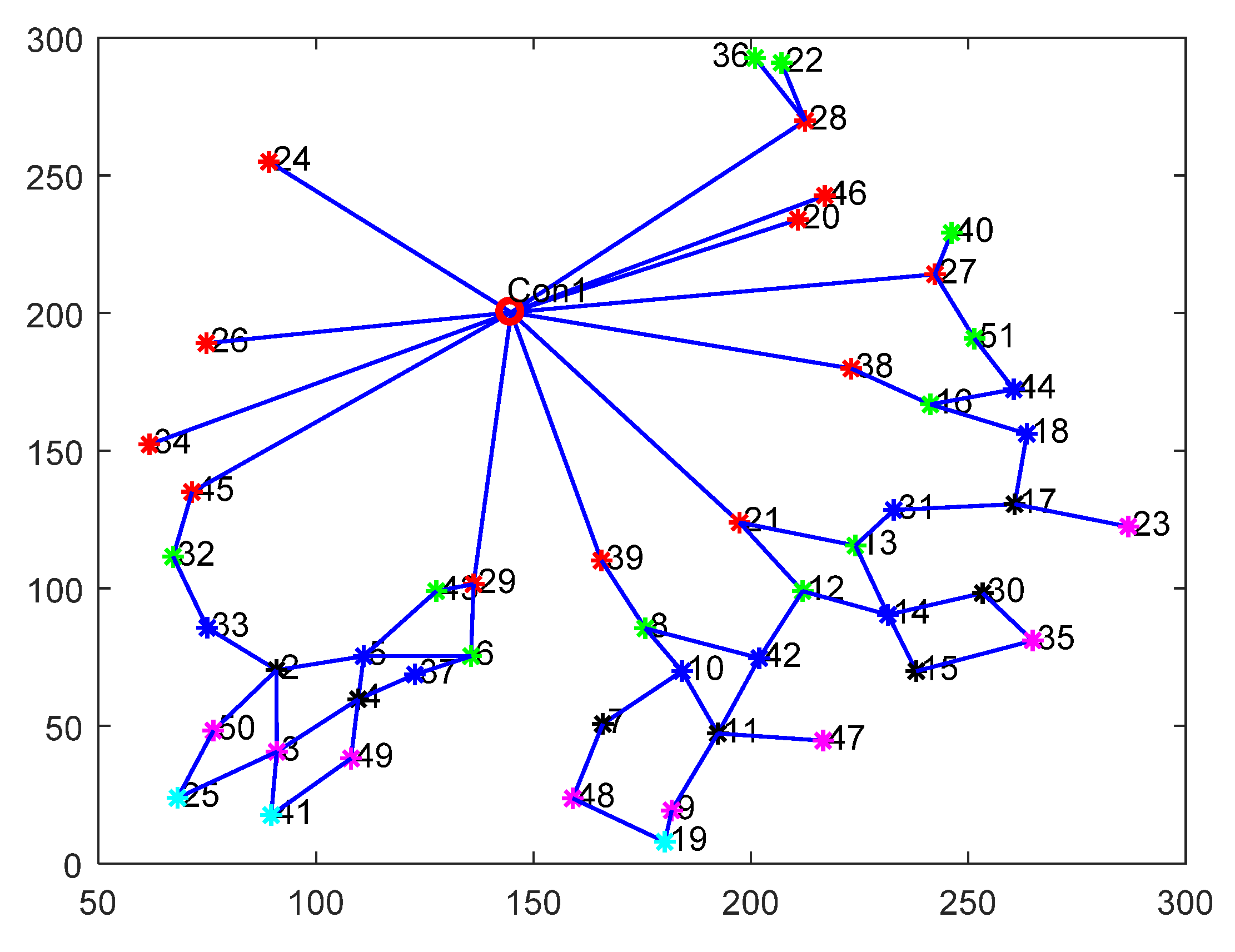
In the same transformer power supply range, the network structure of the smart meter and the concentrator refers to [20], and the data communication network structure in the low voltage distribution network is as shown in Figure 2, where, node 1 is the PLC concentrator, and the other nodes are the smart meters from which date needs to be collected.

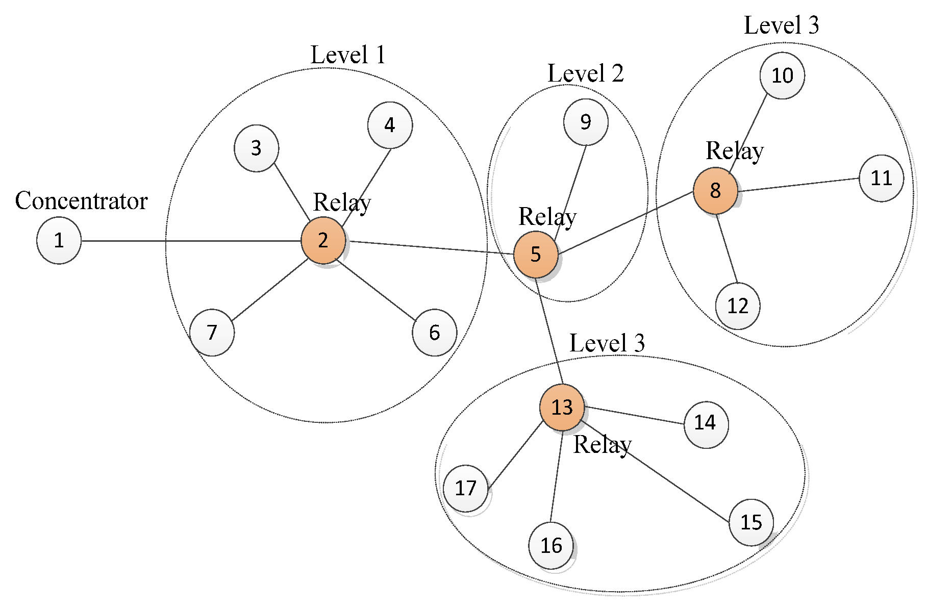
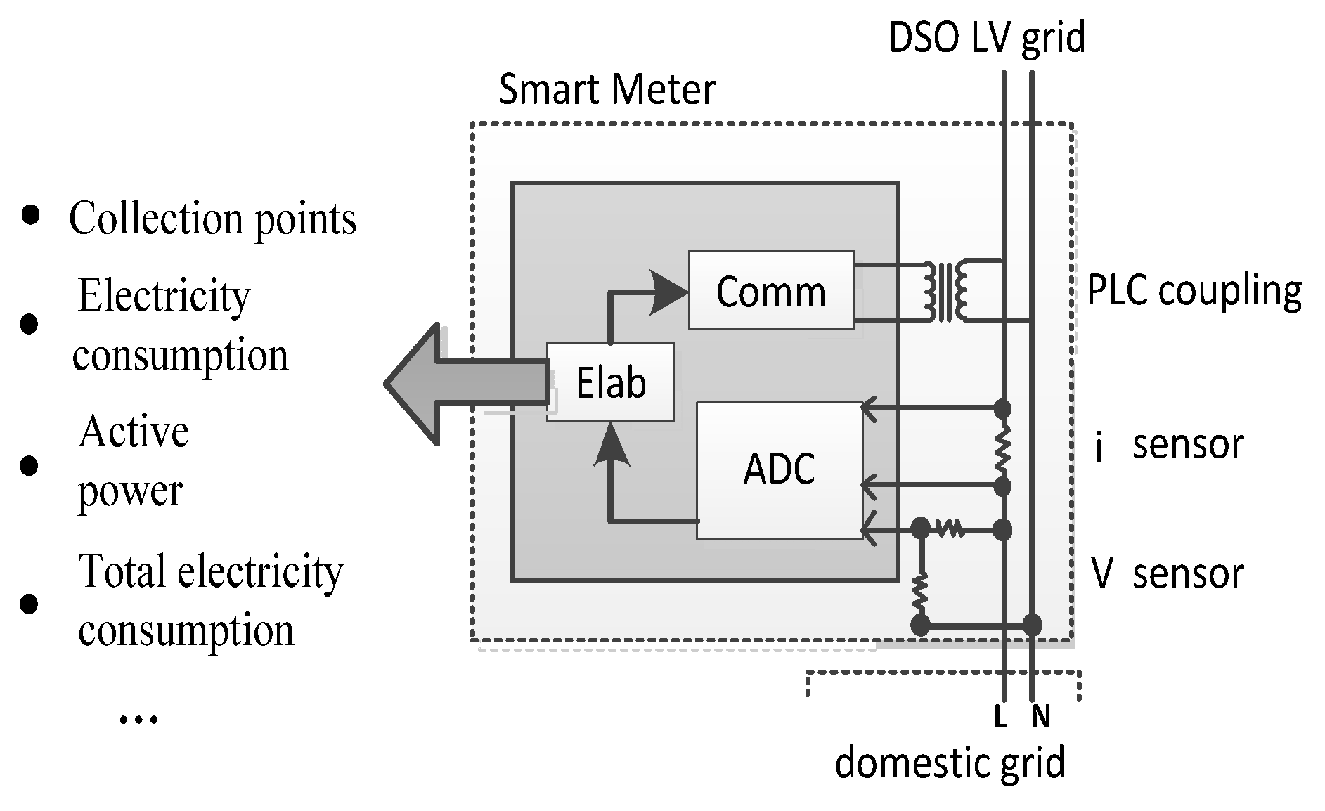
As shown in Figure 3, smart meter devices are typically installed at end-users on the low-voltage (LV) feeders [21], and there is some information that needs to be collected in the ELAB module of the smart meter, such as collection points, electricity consumption and so on.

2.2. Static Relay Selection

The paper divides the logical topology of the smart meters in the experimental area into several sub-networks. The schematic diagram of static relay selection for each sub-network is shown in Figure 4, and the networking steps of the sub-networks are as follows:

(1)

As shown in Figure 2, smart meters that can communicate directly with the PLC concentrator represented by No. 1 are placed in the first-level sub network, and they are used as relays of the first-level sub network, for example, smart meters No. 2, No. 3 and No. 4 all belong to the first-level sub network.

(2)

The smart meters directly connected with the first level relay (direct communication) are placed in the first level sub network, and there are several smart meters in each first level subnet. For example, in Figure 2, the No. 5 and No. 6 smart meters belong to the first-level subnet with No. 2 smart meter as the relay. No. 7 and No. 8 smart meters belong to the first-level subnet with No. 3 smart meter as the relay. No. 9 and No. 10 smart meters belong to the first-level subnet with No. 4 smart meter as the relay.

(3)

If the smart meter that does not belong to the first-level subnet could directly communicate with the smart meter in the first-level subnet, we place it in the second-level subnet and the smart meter in the first-level subnet connected to it is used as the relay of the second-level subnet. For example, No. 11 smart meter in Figure 2 is placed in the second-level subnet with No. 5 smart meter as the relay; No. 12 smart meter is placed in the second-level sub network with No. 6 smart meter as the relay; No. 13 smart meter is placed in the second-level sub network with No. 7 smart meter as the relay; No. 14 smart meter is placed in the second-level sub network with No. 8 smart meter as the relay. If there are multiple first-level smart meters and the same second-level smart meters to communicate, in order to avoid communication failure caused by the signal conflict, the best path is selected referring to Equation (2) below.

(4)

If there is a third-level subnet, a fourth-level subnet, and so on, follow the above steps to continue the hierarchical network until all static relays are selected.

Finally, referring to the logical topology structure between the concentrator and the smart meters within the same transformer power supply range, the hierarchical selection method based on static relay is used to perform relay selection for each level sub-network, so as to prepare for the establishment of the subsequent optimal communication path.

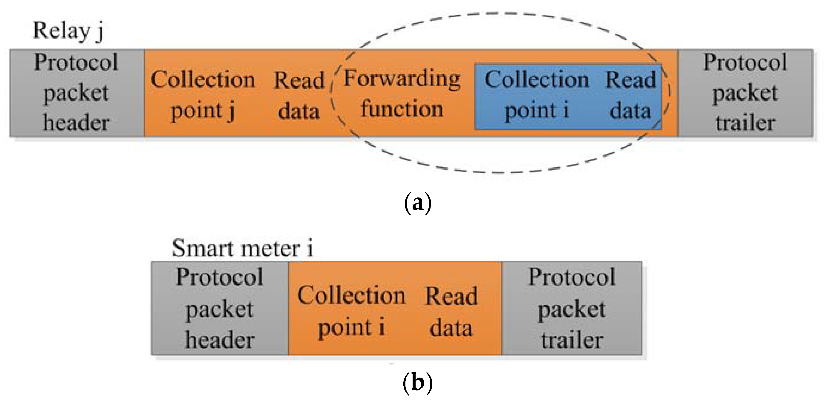
As a relay, the smart meter has the function of transmitting the concentrator’s information and the protocol format that it receives is shown in Figure 5a. The protocol format received by the smart meter that is not selected as relay is shown in Figure 5b. According to the comparison of the protocol format between the relay and the smart meter as is shown in Figure 5, the smart meter selected as the relay has the function of forwarding the message to the next smart meter, but the smart meter not selected as the relay does not have the function of forwarding message.

2.3. Dynamic Relay Selection

When the same smart meter can communicate with multiple relays at the same time, in order to avoid the actual signal conflict problem, the communication link is optimized to ensure that each level subnet has a unique relay. Therefore, in order to establish optimal communication paths between the concentrator and smart meters, this paper introduces the communication quality $Q$ and uses the communication distance between the two smart meters as the communication quality value. The smaller the value of $Q$, the better the communication quality.

It is assumed that the number of smart meters that can communicate directly with the No. $i$ relay is $F_{i,j}$. Set the smart meter number to: $1,2,...i$. The number of smart meters that the No. $i$ relay forward to the superior relay is:

$$F_{i,j}=N_{i,j}+{\displaystyle \sum _{l=1}^{N_{i,j}}{F}_{i,j-1}},$$

(1)

$N_{i,j}$ is the number of the smart meters in the $jth$ level sub network with the No. $i$ smart meter as the relay. $F_{l,j-1}$ is the number of the smart meters in the $(j-1)th$ level sub network with the No. $l$ smart meter as the relay.

When the same smart meter belongs to multiple relay communication ranges, the smart meter performs the best path selection according to the link optimization index, for example, the link optimization index of the number $i$ smart meter relay to the number $k$ smart meter:

$$Y_{i,j-k}=\alpha Q_{i,j-k}+\beta F_{i,j},$$

(2)

where $Y_{i,j-k}$ is the link optimization index between the No. $i$ relay and No. $k$ smart meter that belongs to the $jth$ level sub network. $\alpha$ is a link optimization weighted coefficient, $\beta$ is the weighted coefficient of the number of smart meters that need to be forwarded to a superior, $\alpha +\beta =1$, $\alpha$ and $\beta$ can vary according to the actual situation. In the experiments, the smaller the value of $Y_{i,j-k}$, the better, that is to choose the minimum $Y_{i,j-k}$ value as the optimal communication branch, and close the communication with other relays at the same time.

3. Dynamically Adjusting the Communication Branch According to the Characteristics of the Collected Data

In the experiments, the data collected from the smart meter mainly include collection points, electricity consumption, total electricity consumption, active power, power factor, voltage, current, date and time. When communication links fail to communicate normally due to impedance input, noise interference and other reasons, or when the collected data information is abnormal, we can dynamically adjust the link optimization index according to Equation (2) to select other communication branches, so the accurate judgment of abnormal data information is the key step to ensure the accurate detection of abnormal data information, according to the experimental results, in ensuring the accuracy and running time of optimal detection conditions, the extreme learning machine is used to monitor the collected data in the paper.

3.1. Basic Principles of Extreme Learning Machine (ELM)

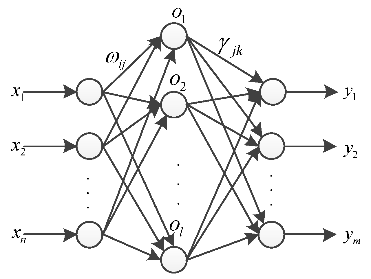
Extreme learning machine has the advantages of fast training and good generalization performance, unlike gradient-based learning algorithms which iteratively adjust network parameters, the weights and biases of the hidden nodes of the ELM are generated randomly. It is a new efficient learning algorithm for single hidden layer feed-forward neural network structure [22]. As is shown in Figure 6, it consists of an input layer, a hidden layer, and an output layer, and the input layer neurons and the hidden layer neurons are all connected, and the hidden layer neurons and the output layer neurons are all connected.

It is assumed that the input layer has $n$ neurons, corresponding to $n$ input variables, the hidden layer has $l$ neurons, the output layer has $m$ neurons, corresponds to $m$ output variables, the connection weight between the input layer and the hidden layer is $\omega$, and the connection weight between the hidden layer and the output layer is $\gamma$:

$$\omega ={\left[\begin{array}{cccc}{\omega }_{11}& {\omega }_{12}& ...& {\omega }_{1n}\\ {\omega }_{21}& {\omega }_{22}& ...& {\omega }_{2n}\\ ⋮& ⋮& ⋮& ⋮\\ {\omega }_{l1}& {\omega }_{l2}& \cdots & {\omega }_{\ln }\end{array}\right]}_{l\times n},$$

(3)

$$\gamma ={\left[\begin{array}{cccc}{\gamma }_{11}& {\gamma }_{12}& ...& {\gamma }_{1m}\\ {\gamma }_{21}& {\gamma }_{22}& ...& {\gamma }_{2m}\\ ⋮& ⋮& ⋮& ⋮\\ {\gamma }_{l1}& {\gamma }_{l2}& ...& {\gamma }_{\ln }\end{array}\right]}_{l\times m},$$

(4)

ω_ji is the connection weight between the i-th neuron of the input layer and the j-th neuron of the hidden layer. γ means the weight of the connection between the j-th neuron of the hidden layer and the k-th neuron of the output layer:

$$b={\left[\begin{array}{cccc}{b}_1& b_2& ...& b_l\end{array}\right]}_{1\times l}^T,$$

(5)

The input matrix X and the output matrix Y of the training are expressed as follows:

$$X={\left[\begin{array}{cccc}{x}_{11}& x_{12}& ...& x_{1Q}\\ x_{21}& x_{22}& ...& x_{2Q}\\ ⋮& ⋮& ⋮& ⋮\\ x_{m1}& x_{m2}& ...& x_{mQ}\end{array}\right]}_{m\times Q},$$

(6)

$$Y={\left[\begin{array}{cccc}{y}_{11}& y_{12}& ...& y_{1Q}\\ y_{21}& y_{22}& ...& y_{2Q}\\ ⋮& ⋮& ⋮& ⋮\\ y_{m1}& y_{m2}& ...& y_{mQ}\end{array}\right]}_{m\times Q},$$

(7)

It is assumed that the activation function of the neurons of the hidden layer is $g(x)$, the output $T$ of the network is listed as follows:

$$T={\left[\begin{array}{cccc}{t}_1,& t_2,& ...,& t_Q\end{array}\right]}_{m\times Q},$$

(8)

$$t_j=\left[\begin{array}{c}{t}_{1j}\\ t_{2j}\\ ⋮\\ t_{mj}\end{array}\right]={\left[\begin{array}{c}{\displaystyle \sum _{i=1}^l{\gamma }_{i1}g({\omega }_i{x}_j+b_i)}\\ {\displaystyle \sum _{i=1}^l{\gamma }_{i2}g({\omega }_i{x}_j+b_i)}\\ ⋮\\ {\displaystyle \sum _{i=1}^l{\gamma }_{im}g({\omega }_i{x}_j+b_i)}\end{array}\right]}_{m\times l},j=1,2,...,Q,$$

(9)

where ${\omega }_i=\left[\begin{array}{cccc}{\omega }_{i1},& {\omega }_{i2},& ...,& {\omega }_{in}\end{array}\right]$; $x_j={\left[\begin{array}{cccc}{x}_{1j},& x_{2j},& ...& x_{nj}\end{array}\right]}^T$.

The activation function used in this paper is listed as follows:

$$g(x)=\{\begin{array}{cc}1& x\ge 0\\ -1& x<0\end{array},$$

(10)

Equation (9) may be expressed as:

$$H\gamma =T^{\prime },$$

(11)

where, $T^{\prime }$ is the transposition of the matrix $T$, and $H$ is the hidden layer output matrix of the neural network.

If the number of the neurons in the hidden layer is equal to the number of the training set samples, it is able to obtain an approximate training sample with zero error for any $\omega$ and $b$ [23]. The formula (12) has been proved in the document [19]:

$${\displaystyle \sum _{j=1}^Q\left|\right|t_j-y_j\left|\right|=0},$$

(12)

where $y_j={[y_{1j},y_{2j},\cdots ,y_{mj}]}^T,j=1,2,\cdots ,Q$.

Referring to [24], the connection weight $\gamma$ between the hidden layer and the output layer can be obtained by solving the least square solution of the equations listed as follows:

$$\underset{\gamma }{\min }\Vert H\gamma -T^{\prime }\Vert ,$$

(13)

$$\stackrel{\wedge }{\gamma }=H^{+}{T}^{\prime },$$

(14)

where $H^{+}$ is the Moore–Penrose generalised inverse [25] of the hidden layer output matrix $H$. There are more details about ELM in [26,27].

3.2. Comparison of Wrapper Feature Selection Algorithms

The increase of input data will cause system redundancy. In order to remove irrelevant data and avoid system redundancy, the paper chooses the most representative subset from a set of known feature sets. The wrapper feature selection algorithm first proposed by John et al. [28,29], has the advantages of high quality of the selected feature, and high classification accuracy when the obtained subset of features is used for classification. In this paper, based on the concept of the wrapper feature selection, we select the characteristics of the data information of the smart meter. The wrapper feature algorithm is bound to a classification algorithm from the beginning to evaluate the quality of the feature by classification, and its formalization formula is listed as (15):

$$\underset{\sigma \in {\left\{0,1\right\}}^n}{\min }G(f^{*},\sigma ,X,Y),s.t\{\begin{array}{c}s(\sigma )\le {\sigma }_0\\ f^{*}=\tilde{T}(F,\sigma ,X,Y)\end{array},$$

(15)

where F is a given classification function, σ is a fixed vector and (X, Y) is the training data. f* is a classification or regression function obtained by learning the model $\tilde{T}$ on the data set X defined by σ. G is used to measure the performance of the classifier f*(σ) on a given set of training sets for a given σ, and G only treats f*(σ) as a black box.

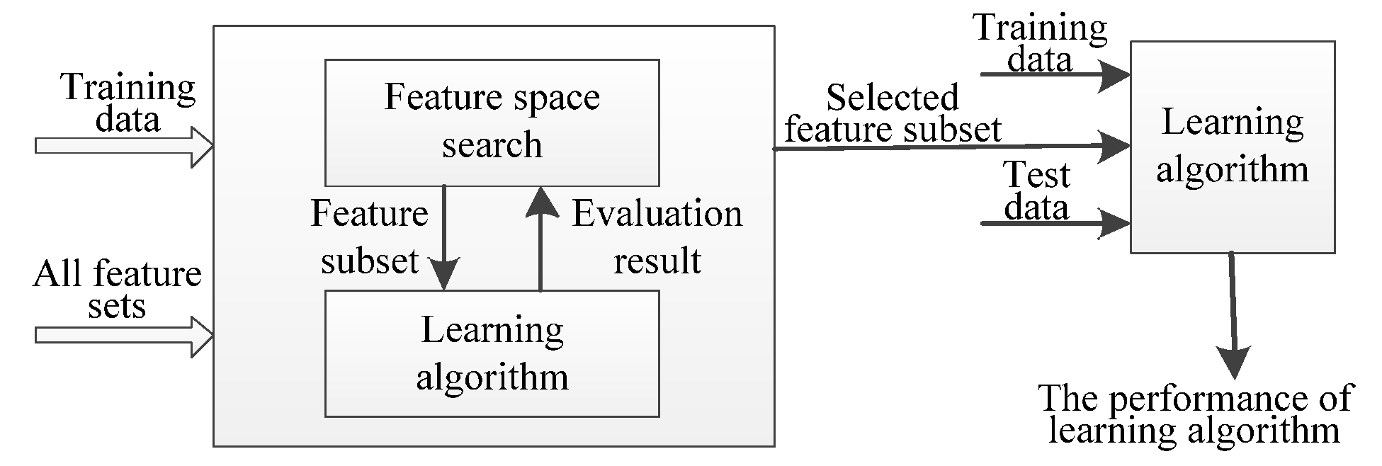
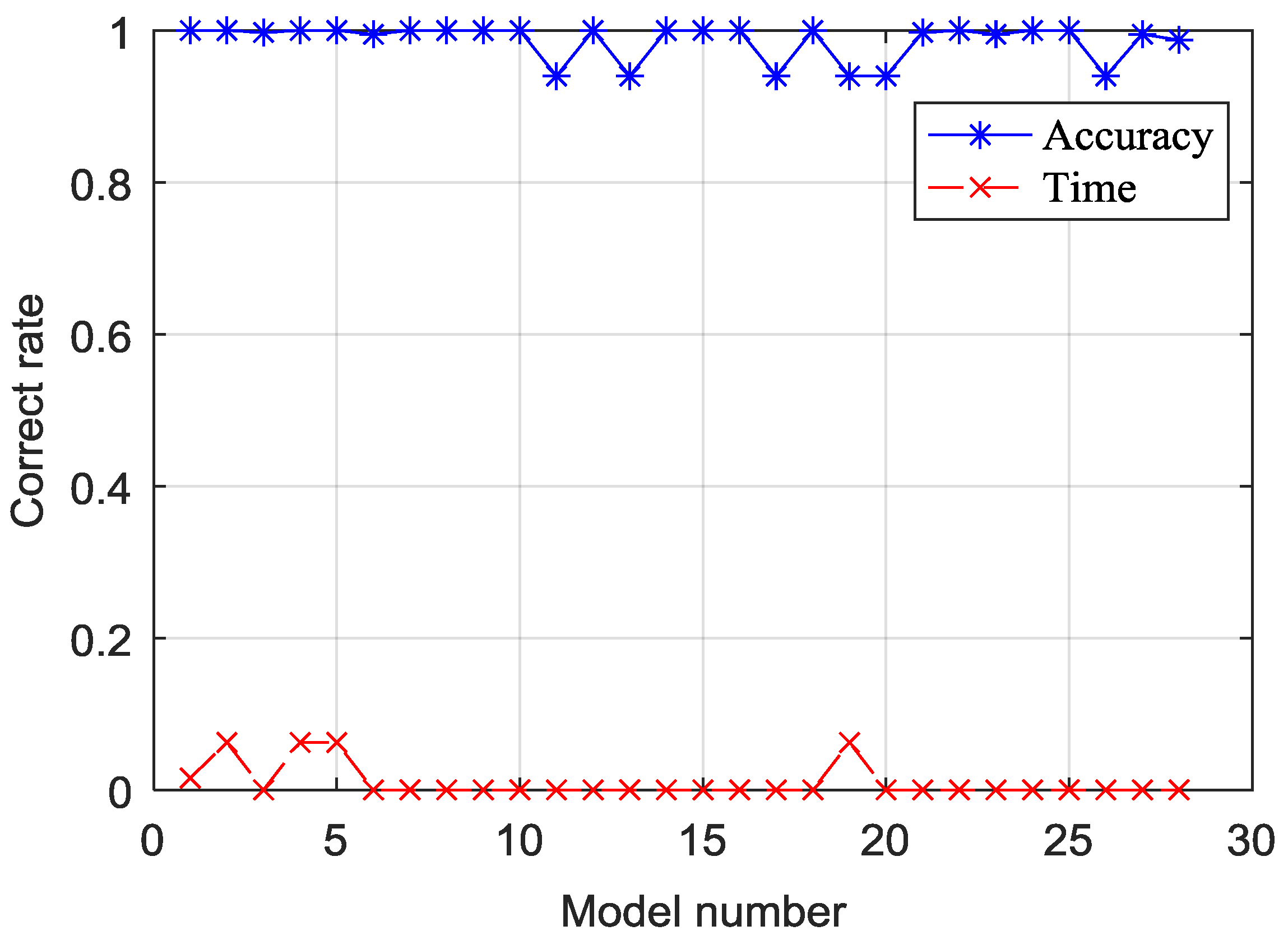
The specific way is to make different combinations of the information feature values, and then select training samples in each combination to train in extreme learning machine, and finally determine the optimal combination by detecting the correct rate and running time of the samples. According to the wrapper feature process which is listed in Figure 7, this paper uses MATLAB to train the extreme learning machine through 910 groups of samples, and the experimental results are shown in Figure 8.

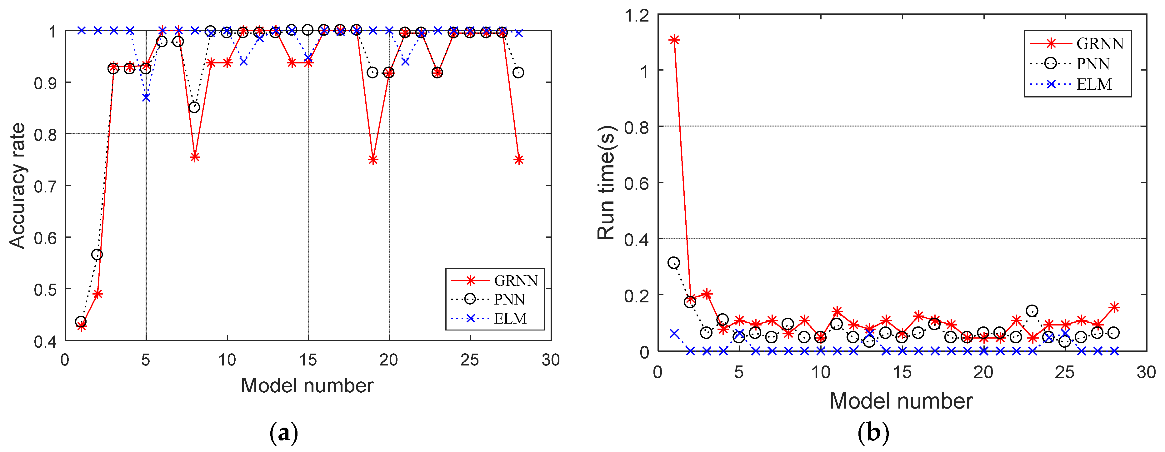
Figure 8 shows that the accuracy of multiple combination models trained by the extreme learning machine reaches 100% while the running time is also minimal. To ensure that the selected feature combination is optimal, referring to the probabilistic neural network (PNN) algorithm which is used for monitoring in [30,31,32] and the generalized regression neural network (GRNN) algorithm which is proposed for use in detection and judgment in [33,34], binding feature selection algorithm experiments with PNN and GRNN are carried out in this paper and the experimental results are shown in Figure 9. From Figure 9, the accuracy of GRNN, PNN, and ELM are all up to 100% at No. 16 and No. 18 models. In practical work, because the concentrator takes electricity usage information from smart meters every 15 min, it needs to consider the running time of the model. From the comparison, under the condition of ensuring the correct rate, the operation speed of ELM is fastest.

3.3. Spatial Distribution of Selected Feature Data

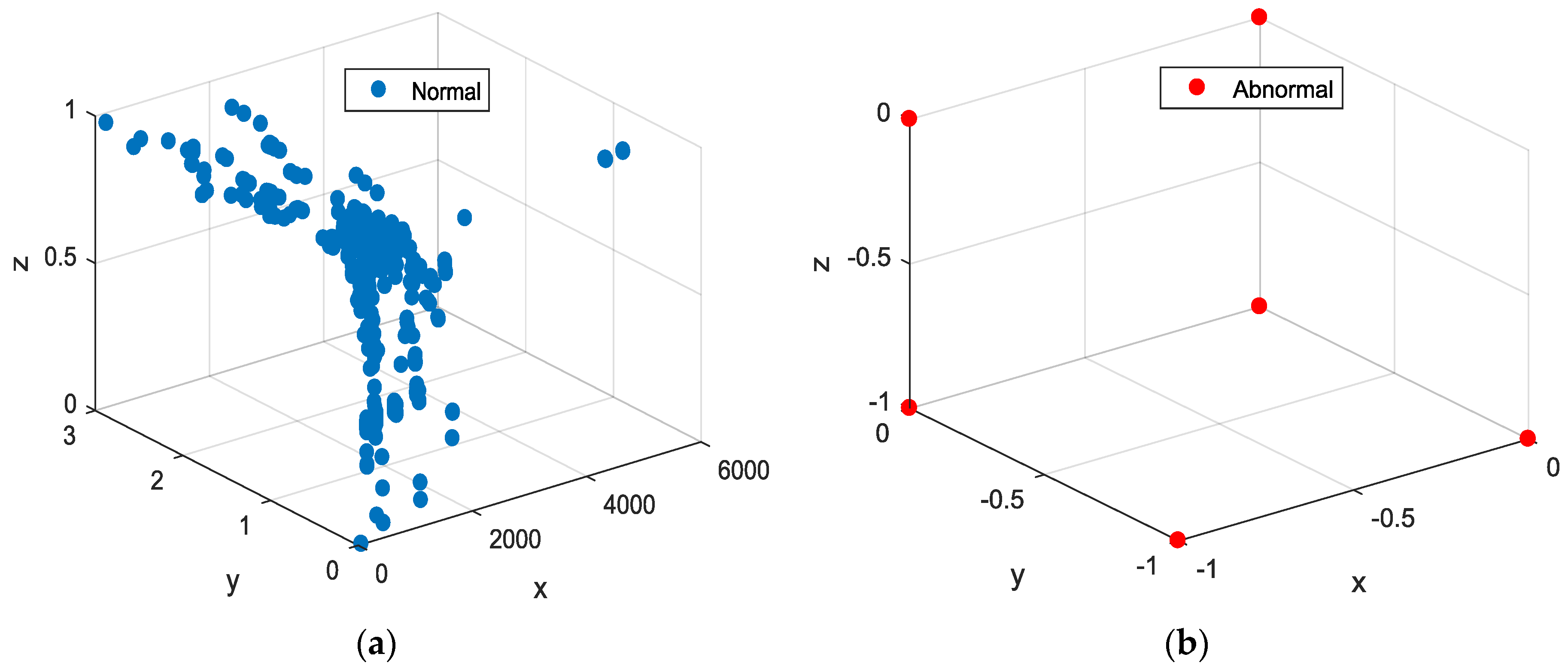
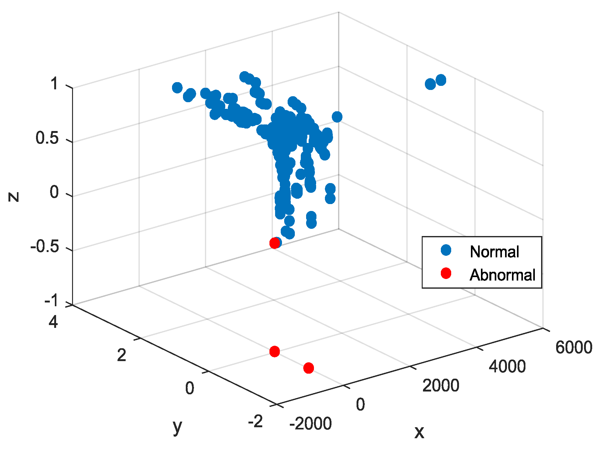
In Figure 9, this paper selects feature values from the sixteenth and eighteenth combination models, and the characteristics of the sixteenth combination models include total electricity consumption, active power, and power factor. The characteristics of eighteenth combination models are total electricity consumption, active power, power factor, voltage, and current. Taking into account the factor of system redundancy, the sixteenth combination has fewer characteristic values. Therefore, this paper selects the sixteenth combination as the characteristics of the electricity usage information and the distribution in three-dimensional space is as shown in Figure 10. Figure 11 gives the distribution of normal data and abnormal data respectively of the sixteenth feature combination model. In the Figure 11, the abnormal data is fixed in six locations, and without data processing, it can be quickly identified.

3.4. The Selection of the Number of Neurons in the Hidden Layera

The selected feature combination is reentered into ELM for training, and it is found that the prediction accuracy of the test set will change with the number of the hidden layer neurons. When the number of neurons in the hidden layer is equal to the number of training samples, ELM can approximate all training samples with zero error [23]. However, in the experiments, more number of neurons in the hidden layer was not better, and sometimes there was a tendency to decrease. 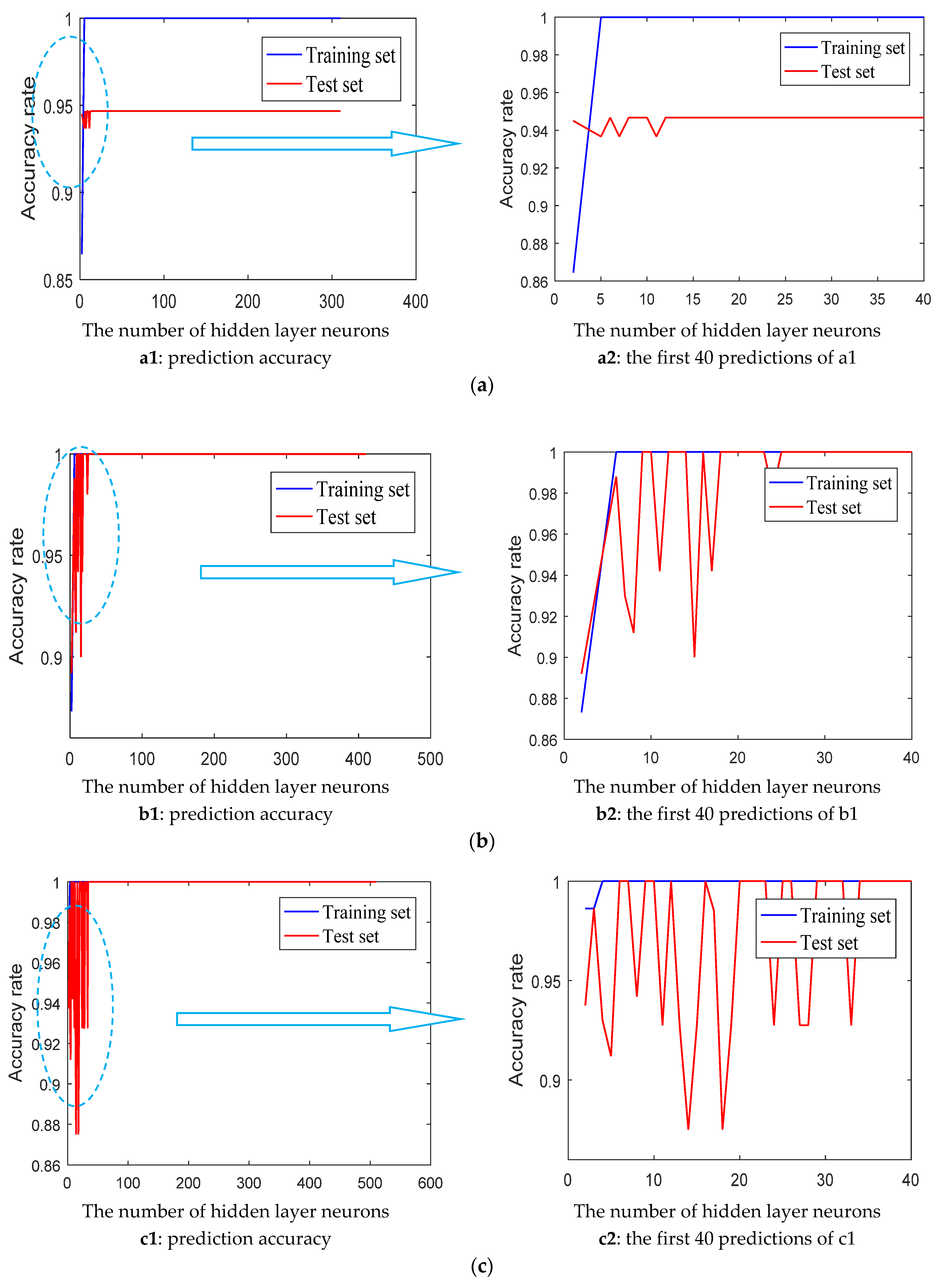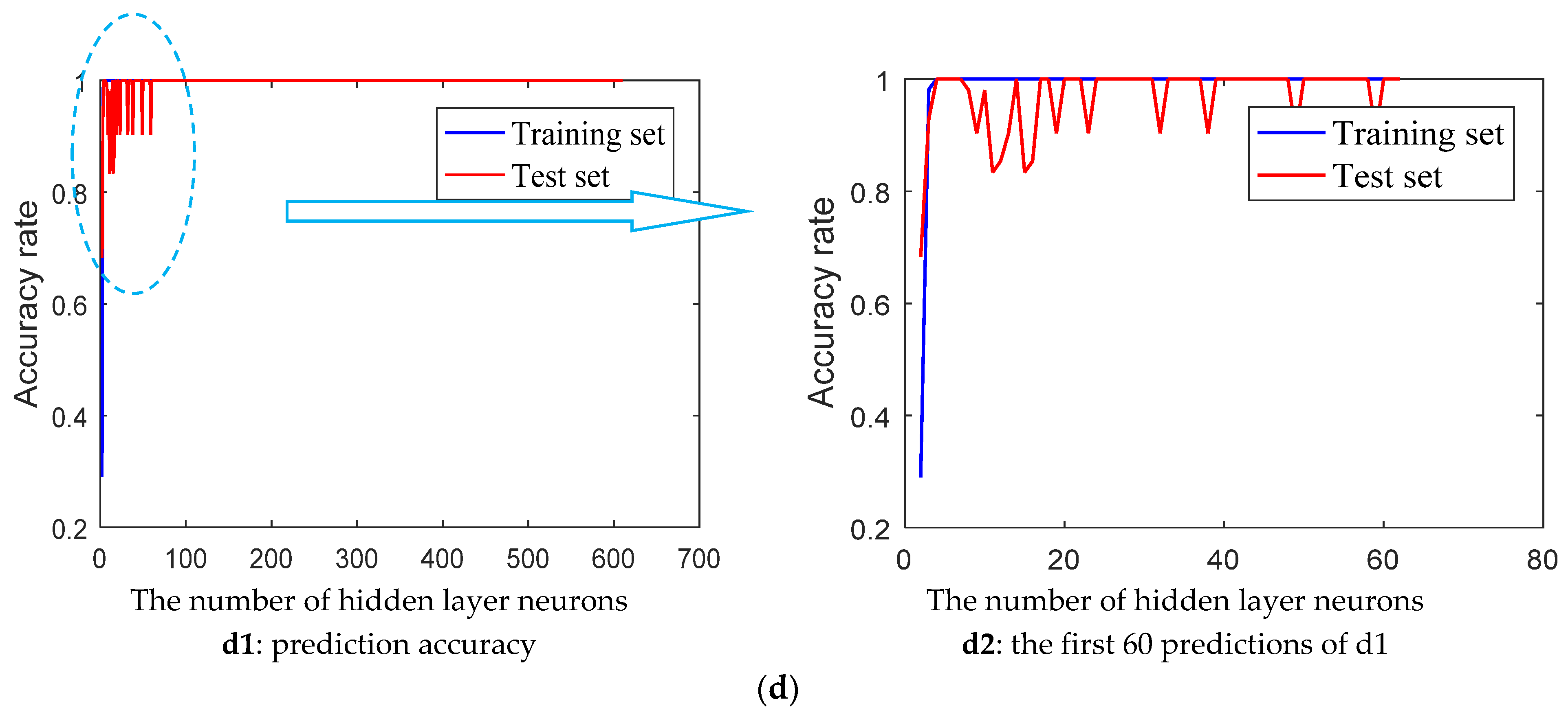Figure 12 lists four different sets of training samples, and the prediction accuracy of the training set and test set varies with the number of neurons in the hidden layer. Therefore, in order to identify the abnormal signal more accurately, the accuracy of the training set and the test set is considered in this paper, and the number of suitable hidden layer neurons is selected.

In Figure 12, (a) is the forecast of 310 training samples and 600 test samples, (b) is the forecast of 410 training samples and 500 test samples, (c) is the forecast of 510 training samples and 400 test samples, (d) is the forecast of 610 training samples and 300 test samples. The training sample could approximate all training samples with zero error when the number of neurons in the hidden layer is small. However, when the number of neurons in the hidden layer is less than 100, the prediction accuracy rate will be in a concussion as the number of hidden neurons increases. Considering the speed of system operation, the number of neurons in the hidden layer is set to 30 in this paper.

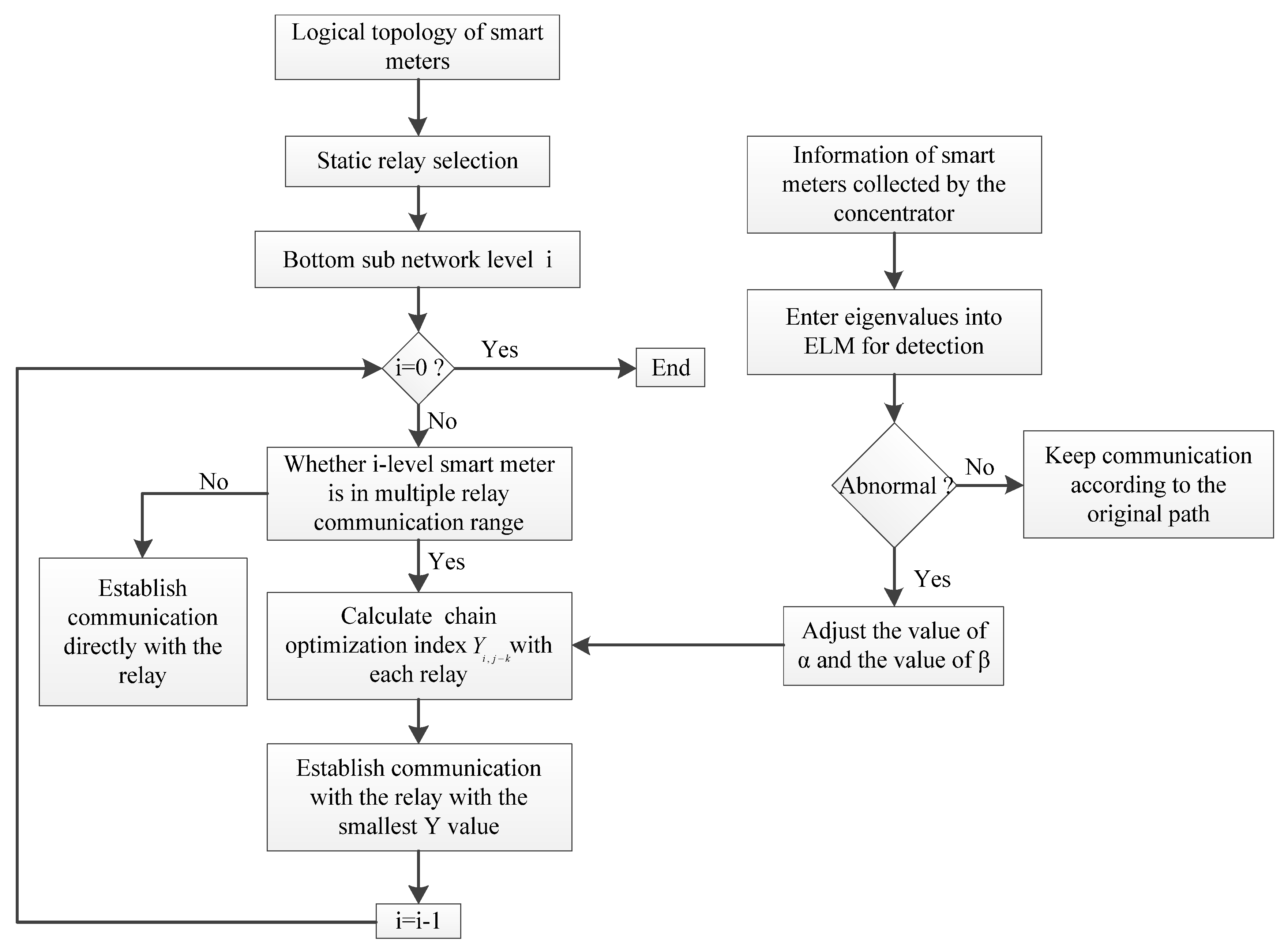
4. Simulation Experiment of Dynamic Adjustment of Communication Branch

The overall experimental procedure refers to Figure 13, and in this paper, Matlab is used to simulate the dynamic adjustment of the communication branch. Figure 14 is the logical topology between the concentrator and the smart meters. Figure 15 is a logical topology based on the selection method of static relay routing where the same color is the smart meter with the same level subnet.

In Figure 15, red represents the smart meter that belongs to the first-level subnet, green is the smart meter belonging to the second-level subnet, blue is the smart meter belonging to the third-subnet, purple is the smart meter belonging to the fourth-level subnet, cyan is the smart meter belonging to the fifth-level subnet. According to the principle of static relay selection, the same level smart meters do not communicate with each other, so there is no communication branch between the same level smart meters on the logical topology. As shown in Figure 15, after the static selection of the relay, the communication between the smart meters in the same sub network is closed, thus reducing the communication branches between the same sub networks, greatly reducing the number of subsequent optimal paths, speeding up the computation speed and improving the system efficiency. However, as can be seen from Figure 15, smart meters: No. 2, No. 3, No. 4, No. 14, No. 17, No. 19, No. 25, No. 41 and No. 44 are all in the communication range of two superior smart meters at the same time. In order to avoid the communication failure caused by the signal conflict, it uses the above method of dynamic relay selection to dynamically network from the low-level sub network to the high-level sub network. According to the actual situation, the link optimization weighting coefficient for each level subnet and the weight coefficient of the number of smart meter that is relayed to the higher level are all different. In this paper, the weight coefficients of subnets at all levels are calculated according to

Table 1. $\alpha$ and $\beta$ values of subnets at all levels.

First Level Subnet		Second Level Subnet		Third Level Subnet		Fourth Level Subnet		Fifth Level Subnet
$\alpha$	$\beta$	$\alpha$	$\beta$	$\alpha$	$\beta$	$\alpha$	$\beta$	$\alpha$	$\beta$
0.70	0.30	0.75	0.25	0.80	0.20	0.90	0.10	0.99	0.01

.

Referring to the logical topology of Figure 15, in the process of dynamic selection of relays from the lowest subnet, when the smart meter has multiple relays to communicate with it, it chooses the smallest link optimization index as the optimal communication path.

Table 2. Dynamic relay link optimization index.

Subnets	Communication Link	$\mathit{F}$	$\mathit{Y}$
Fifth level subnet	25-50	1	25.5286
	25-3	2	28.0120
	41-3	2	22.7859
	41-9	1	27.2615
	19-48	1	26.1475
	19-9	1	11.4238
Fourth level subnet	2-33	3	18.2742
	2-5	7	17.9471
	4-5	7	14.3206
	4-37	4	13.6763
	11-10	5	20.2870
	11-42	4	24.0006
	17-31	2	26.8972
	17-18	2	23.3184
Third level subnet	5-43	4	22.9051
	5-6	9	21.1908
	42-8	8	22.5131
	42-12	5	20.9748
	14-12	8	18.0438
	14-13	5	20.8795
	44-16	4	15.9352
	44-51	1	15.6752

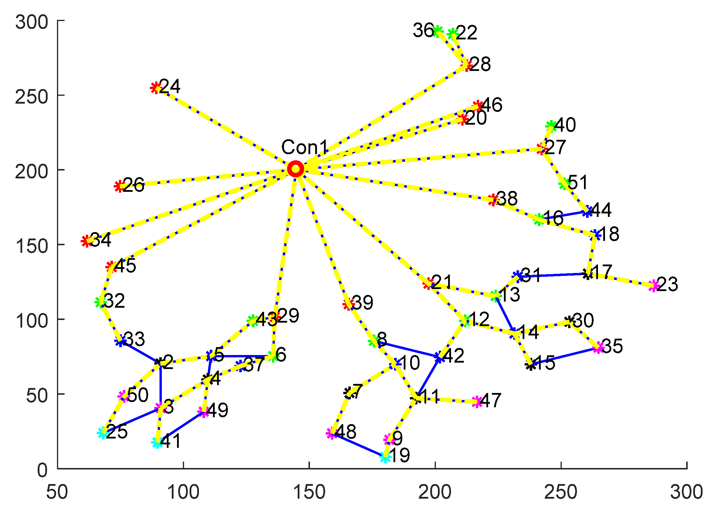
shows the link optimization values $Y$ for the smart meters that can communicate with multiple superiors at the same time and the number $F$ of smart meters that the selected relay needs to relay to the superior. Figure 16 is the communication path of all smart meters after dynamic selection based on Table 2, and the yellow connection line represents the final communication path. In order to prevent signal conflicts, the blue line is closed.

According to the characteristics of the electricity usage information, it could dynamically adjust the link optimization weighting coefficient $\alpha$ and the weighting coefficient $\beta$ of the number of the smart meter to relay to the superior, so as to establish other communication paths quickly. For example, when the data of the No. 44, No. 4, No. 25 and No. 11 smart meters are abnormal, reduce the inter link optimization weighting coefficient $\alpha$, and increase the weighting coefficient $\beta$ at the same time. Recalculate the link optimization index $Y$ according to Equation (2) above and then the communication path of 44-46-38-1, the communication path of 4-5-43-29-1, the communication path of 25-3-4-37-6-29-1 and the communication path of 11-42-12-21-1 are chosen as the optimal links to communicate, which can find out the optimal communication path quickly and timely, and increase the reliability of data communication for the next time.

5. Conclusions

In order to ensure the accurate collection of smart meter information, and to overcome the problem of signal conflict in the process of smart meter networking and the continued abnormality of information being collected from a certain smart meter, this paper adopts the idea of static and dynamic combination and the method of dynamically adjusting the communication path according to the characteristics of power consumption information to network the smart meters. This paper classifies the smart meters referring to the logical topology structure of the smart meters in the experimental area and selects an appropriate smart meter as the relay for each sub-network. If the same smart meter belongs to communication range of multiple relays, the optimal relay is selected for communication according to the principle proposed in this paper that the smaller of link optimization index, the better. Because of the uniqueness of the relay, it can effectively avoid the signal conflict in the process of smart meter communication. In addition, in the process of collecting information, the ELM can quickly detect abnormal information. Then, by adjusting the chain optimization weighted coefficient $\alpha$ and the weighted coefficient $\beta$ of the number of the relayed smart meters, a new communication path can be found, which can effectively prevent the continuous abnormality of the smart meter information. The networking method proposed in this paper solves some problems existing in current smart meter networking, thereby improving the reliability of smart meter communication and ensuring the accurate collection of smart meter information. In practical work, there are some issues that need to be further studied:

(1)

The logical topology of smart meter communication is complex. The research in this paper is carried out under the condition that the logical topology structure is known. Therefore, the logical topology structure between the concentrator and the smart meters can be studied later.

(2)

In the process of dynamic networking, this article mainly considers the communication quality and relay forwarding number. However, in practice, the time-varying power line channel has a great influence on the communication quality in the networking process, and the time-varying power line channel can be introduced into the dynamic networking for further research.

References

- Bahrami, S.; Wong, V.W. An Autonomous Demand Response Program in Smart Grid with Foresighted Users. In Proceedings of the IEEE Smart Grid Communications, Miami, FL, USA, 2–5 November 2015; pp. 205–210. [Google Scholar] [CrossRef]
- Amini, M.H.; Frye, J.; Ilić, M.D.; Karabasoglu, O. Smart Residential Energy Scheduling Utilizing Two Stage Mixed Integer Linear Programming. In Proceedings of the North American Power Symposium (NAPS), Charlotte, NC, USA, 4–6 October 2015; pp. 1–6. [Google Scholar] [CrossRef]
- Bahrami, S.; Wong, V.W.; Huang, J. An Online Learning Algorithm for Demand Response in Smart Grid. Trans. Smart Grid 2017. [Google Scholar] [CrossRef]
- Amini, M.H.; Nabi, B.; Haghifam, M.R. Load Management Using Multi-agent Systems in Smart Distribution Network. In Proceedings of the IEEE Power and Energy Society General Meeting, Vancouver, BC, Canada, 21–25 July 2013; pp. 1–5. [Google Scholar] [CrossRef]
- Tian, S.; Luan, W.; Zhang, D.; Liang, C.; Sun, Y. Technical Forms and Key Technologies on Energy Internet. Proc. CSEE 2015, 35, 3482–3494. [Google Scholar] [CrossRef]
- Yu, K.; Yong, J.; Liang, S.; Tian, Q. An Improved Power Line Signaling Technique Based Anti-islanding Protection Approach for Distributed Generation System. Proc. CSEE 2015, 35, 3283–3291. [Google Scholar] [CrossRef]
- Khalil, K.; Gazalet, M.G.; Corlay, P.; Coudoux, F.X.; Gharbi, M. An MIMO Random Channel Generator for Indoor Power-line Communication. IEEE Trans. Power Deliv. 2014, 29, 1561–1568. [Google Scholar] [CrossRef]
- Li, J.; Jia, Z.; Zhang, T.; Zeng, L. Network Construction Method of Cable Anti-theft Network Based on Improved Ant Colony Algorithm. J. Chongqing Univ. Technol. 2017, 31, 160–165. [Google Scholar]
- Mishra, M.; van Riet, M. A Channel Model for Power Line Communication Using 4PSK Technology for Diagnosis: Some Lessons Learned. Int. J. Electr. Power Energy Syst. 2018, 95, 617–634. [Google Scholar] [CrossRef]
- Cao, W.; Yin, C.; Xie, Z.; Liang, X.; Li, X. Research on Broadband MIMO Power Line Communications Model. Proc. CSEE 2017, 37, 1136–1141. [Google Scholar] [CrossRef]
- Zimmermann, M.; Dostert, K. A Multipath Model for the Power Line Channel. IEEE Trans. Commun. 2002, 50, 553–559. [Google Scholar] [CrossRef]
- Qi, J.; Liu, X.; Xu, D.G.; Li, Y.; Mou, Y.F. Simulation Study on Cluster-based Routing Algorithm and Reconstruction Method of Power Line Communication Over Lower-voltage Distribution. Proc. CSEE 2008, 28, 65–71. [Google Scholar] [CrossRef]
- Liu, X.; Zhang, L.; Zhou, Y.; Xu, D. Performance Analysis of Power Line Communication Network Model Based on Spider Web. In Proceedings of the IEEE 8th International Conference on Power Electronics and ECCE Asia (ICPE & ECCE), Jeju, Korea, 30 May–3 June 2011; pp. 953–959. [Google Scholar]
- Liu, X.; Zhang, L.; Zhou, Y.; Qi, J.; Huang, N. Performance Analysis of Novel Low-voltage Power Line Communication Model. Trans. China Electrotech. Soc. 2012, 27, 271–277. [Google Scholar] [CrossRef]
- Su, H.; Shi, J.; Liang, Z.; Wu, C. Automatic Transmission Line Path Selection Based on GIS and Improved CA. Electr. Power Autom. Equip. 2016, 36, 109–114. [Google Scholar] [CrossRef]
- Ran, Q.; Wu, Y.; Qi, M. Research on Automatic Routing Method of Low-voltage Power Line Carrier Network. Power Syst. Prot. Control 2011, 39, 53–63. [Google Scholar]
- Chen, K.; Hu, X. Method of relay routing based on genetic adaptive ant colony system algorithm. J. Central South Univ. 2013, 44, 571–579. [Google Scholar]
- Xing, N.; Zhang, S.; Shi, Y.; Guo, S. PLC-oriented Access Point Location Planning Algorithm in Smart-grid Communication Networks. China Commun. 2016, 13, 91–102. [Google Scholar] [CrossRef]
- Wang, Y.; Xue, C.; Jiao, Y. Hierarchical Classification PLC Routing Algorithm Combinating Static Relay With Dynamic Relay in Medium Voltage Distribution Network. Electr. Power Autom. Equip. 2017, 37, 8–15. [Google Scholar] [CrossRef]
- Navarro-Espinosa, A.; Mancarella, P. Probabilistic Modeling and Assessment of the Impact of Electric Heat Pumps on Low Voltage Distribution Networks. Appl. Energy 2014, 127, 249–266. [Google Scholar] [CrossRef]
- Ni, F.; Nguyen, P.H.; Cobben, J.F.G.; Van den Brom, H.E.; Zhao, D. Three-phase State Estimation in the Medium-voltage Network With Aggregated Smart Meter Data. Int. J. Electr. Power Energy Syst. 2018, 98, 463–473. [Google Scholar] [CrossRef]
- Khosravi, V.; Ardejani, F.D.; Yousefi, S.; Aryafar, A. Monitoring Soil Lead and Zinc Contents via Combination of Spectroscopy with Extreme Learning Machine and Other Data Mining Methods. Geoderma 2018, 318, 29–41. [Google Scholar] [CrossRef]
- Feng, G.; Huang, G.B.; Lin, Q.; Gay, R. Error Minimized Extreme Learning Machine with Growth of Hidden Nodes and Incremental Learning. IEEE Trans. Neural Netw. 2009, 20, 1352–1357. [Google Scholar] [CrossRef] [PubMed]
- Yeom, C.U.; Kwak, K.C. Short-Term Electricity-Load Forecasting Using a TSK-Based Extreme Learning Machine with Knowledge Representation. Energies 2017, 10, 1613. [Google Scholar] [CrossRef]
- Serre, D. Matrices: Theory and Application; Springer: New York, NY, USA, 2002. [Google Scholar]
- Zhu, Q.Y.; Qin, A.K.; Suganthan, P.N.; Huang, G.B. Evolutionary Extreme Learning Machine. Pattern Recogn. 2005, 38, 1759–1763. [Google Scholar] [CrossRef]
- Huang, G.B.; Zhu, Q.Y.; Siew, C.K. Extreme Learning Machine: Theory and Applications. Neurocomputing 2006, 70, 489–501. [Google Scholar] [CrossRef]
- John, G.H.; Kohavi, R.; Pfleger, K. Irrelevant Features and the Subset Selection Problem, Machine Learning. In Proceedings of the Eleventh International Conference, Rutgers University, New Brunswick, NJ, USA, 10–13 July 1994; pp. 121–129. [Google Scholar]
- Kohavi, R.; John, G.H. Wrappers for Feature Subset Selection. Artif. Intell. 1997, 97, 273–324. [Google Scholar] [CrossRef]
- Teles, L.O.; Fernandes, M.; Amorim, J.; Vasconcelos, V. Video-tracking of Zebrafish (Danio rerio) as A Biological Early Warning System Using Two Distinct Artificial Neural Networks: Probabilistic Neural Network (PNN) and Self-organizing Map (SOM). Aquat. Toxicol. 2015, 165, 241–248. [Google Scholar] [CrossRef] [PubMed]
- Ali, J.B.; Saidi, L.; Mouelhi, A.; Chebel-Morello, B.; Fnaiech, F. Linear Feature Selection and Classification Using PNN and SFAM Neural Networks for A Nearly Online Diagnosis of Bearing Naturally Progressing Degradations. Eng. Appl. Artif. Intell. 2015, 42, 67–81. [Google Scholar] [CrossRef]
- Hajmeer, M.; Basheer, I. A Probabilistic Neural Network Approach for Modeling and Classification of Bacterial Growth/no-growth Data. J. Microbiol. Methods 2002, 51, 217–226. [Google Scholar] [CrossRef]
- Modaresi, F.; Araghinejad, S.; Ebrahimi, K. A Comparative Assessment of Artificial Neural Network, Generalized Regression Neural Network, Least-square Support Vector Regression, and K-nearest Neighbor Regression for Monthly Streamflow Forecasting in Linear and Nonlinear Conditions. Water Resour. Manag. 2018, 32, 243–258. [Google Scholar] [CrossRef]
- Ye, H.; Ren, Q.; Hu, X.; Lin, T.; Shi, L.; Zhang, G.; Li, X. Modeling Energy-related CO2 Emissions from Office Buildings Using General Regression Neural Network. Resour. Conserv. Recycl. 2018, 129, 168–174. [Google Scholar] [CrossRef]
© 2018 by the authors. Licensee MDPI, Basel, Switzerland. This article is an open access article distributed under the terms and conditions of the Creative Commons Attribution (CC BY) license (http://creativecommons.org/licenses/by/4.0/).