Boundary Conditions Accuracy Effect on the Numerical Simulations of the Thermal Performance of Building Elements

Abstract

Numerical simulation is widely used in the field of computational building physics for the definition of the thermal performance of building elements. An integral component of numerical simulation using finite elements is the boundary conditions, which, in the case of simulating the thermal performance of a building element, are usually expressed in terms of the external surface temperature as a function of time. The purpose of this study is to examine the effect of the accuracy of the boundary conditions on the thermal performance simulation of building elements. The assumption that the temperature versus time is a sinusoidal function, applied in standard methods, is comparatively assessed with the actual function for diverse climatic conditions using finite elements simulation. The findings of the analysis indicate that the sinusoidal function fails to accurately simulate real boundary conditions. The originality of this study lies within the adoption of a signal reconstruction algorithm, which follows a novel approach by reconstructing the actual temperature versus time signal for the simulation of the actual boundary conditions.

1. Introduction

Heat transfer problems are, in general, classified as steady state or transient. The term “steady” implies no change with time at any point within the medium, while the term “transient” implies variation with time or time dependence. The heat flux remains unchanged with time in cases of steady heat transfer modelling through a medium at any location, although it may vary from one location to another. The quasi-steady-state methods calculate the heat balance over a sufficiently long time, while the transient methods calculate the heat balance using short times steps, taking into account the heat stored in and released from the mass of the building.

Concerning the energy performance of buildings, a steady-state calculation gives the correct results on an annual basis; however, estimates for individual months often have large relative errors [1]. According to the findings of previous studies, a large gap exists between the average values of the calculated and the measured energy in cases where steady-state calculation methods have been applied. In some cases, the ratio between the calculated and the measured energy was found to exceed 4 [2]. In transient heat transfer, the temperature normally varies with time, as well as position. Most heat transfer problems encountered in practice are transient in nature, however, they are usually analyzed under some presumed steady conditions as steady processes are computationally less expensive to simulate.

In the case of heat transfer in building elements, the two principal factors relating to the external thermal environment are the outdoor air temperature and the solar radiation intensity [3]. Both of these are subject to erratic fluctuations and, therefore, steady-state heat transmission seldom occurs in the outside walls of a building. Regarding the internal thermal conditions, these are usually regulated by heating ventilating and air-conditioning (HVAC) systems and, as such, they can be considered as constant. Dynamic methods may facilitate the calculation of heat transmission using specific schedules, such as temperature set-points, outdoor climatic conditions, ventilation modes, etc. Dynamic methods produce time resolved results, ensuring accuracy and applicability for a buildings dynamic thermal behavior.

According to ISO 13786:2007 [4], the variations of the external temperature and heat flows through a building element vary sinusoidally with time around their long term average values. This is also the practice followed in numerous scientific studies in the literature. However, the temperature sinusoidal function assumption is a hypothesis which is not accurate. Specifically, the assumptions of the existing methodology framework for a buildings dynamic thermal behavior have the following drawbacks.

The sinusoidal function of time of the external temperature is a simplified approach as it does not consider nonlinearities such as the temperature dependence of the thermal conductivity and radiation boundary conditions.

The current applied practice poses particular problems for the accuracy of the estimates due to the fact that not all heat transfer mechanisms are thoroughly considered. With the exception of steady one-dimensional or transient heat conduction problems, all heat transfer problems result in partial differential equations, and solving such equations usually requires mathematical methods such as orthogonality, eigenvalues, Fourier and Laplace transforms, Bessel and Legendre functions, and infinite series. A further objection is often made concerning the penetration depth of the material layers and the one dimensional approach.

The purpose of this study is to examine the impact of the sinusoidal temperature boundary condition assumption on the accuracy of the results obtained by numerical simulation for the thermal performance of building elements, and to introduce an improved model for the definition of the boundary temperature. In Section 2, the theoretical background of the existing methodology framework for a buildings dynamic thermal behavior and the current practices found in the literature are described. In Section 3 the methods and the case studies examined in this study are presented. Section 4 presents the comparative assessment of the heat flux within a building element for both actual and sinusoidal boundary conditions using finite element heat transfer simulation. In Section 5, a signal reconstruction algorithm is used to define an improved algorithm for the definition of the temperature boundary conditions for the simulation of the actual external temperature for diverse climatic conditions.

2. Theoretical Background

2.1. Boundary Conditions in Standardized Methods

EN Standard 13786:2007 [4] entitled “Thermal performance of building components—Dynamic thermal characteristics—Calculation methods” provides a means to assess the contribution that building products and services make to energy conservation and to the overall energy performance of buildings. This standard describes the dynamic thermal characteristics of a building component when it is subject to variable boundary conditions, i.e., a variable heat flow rate or variable temperature at one or both of its boundaries. In this International Standard, only sinusoidal boundary conditions are considered: boundaries are subject to sinusoidal variations of temperature or heat flow rate. The variations of the temperature and heat flows around their long-term average values vary are described by a sine function with time:

$$T_n\left(t\right)=\overline{T_n}+\left|\widehat{T_n}\right|cos\left(\omega t+\psi \right)=\overline{T_n}+\frac{1}{2}\left[{\widehat{T}}_{+n}{e}^{j\omega t}+{\widehat{T}}_{-n}{e}^{-j\omega t}\right],$$

(1)

$$Q_n\left(t\right)=\overline{Q_n}+\left|{\widehat{Q}}_n\right|cos\left(\omega t+\psi \right)=\overline{Q_n}+\frac{1}{2}\left[{\widehat{Q}}_{+n}{e}^{j\omega t}+{\widehat{Q}}_{-n}{e}^{-j\omega t}\right].$$

(2)

2.2. Boundary Condition Common Practices in the Literature

The numerical simulation studies found in the literature for the investigation of the thermal performance of building elements fall into two categories: those approaching the boundary temperature as a sinusoidal function versus time, and those applying real local meteorological data to model the exterior temperature. Based on this categorization, this section reviews a selection of numerical simulation studies of buildings and building elements.

Kontoleon and Eumorfopoulou [5], Zhang and Wachenfeldt [6], Viot et al. [7], and Yang et al. [8] employed sinusoidal functions to model the fluctuations in the exterior temperature over time. The outside environmental data in Kontoleon and Eumorfopoulou [5] correspond to the mild Mediterranean climate, which can be represented by a steady pattern with approximately the same diurnal average over a period of several days. The temperatures of the outdoor environment were varied from 22 °C to 30 °C, while the selected desired indoor temperature was 24 °C. In Zhang and Wachenfeldt [6], a sinusoidal temperature profile fluctuating between 20 °C and 30 °C over a period of 5 days was applied, with the initial temperature for all of the models set to 20 °C. The heat transfer coefficient between the wall surface and the media temperature was calculated according to the standard EN 15265:2007 as 8 W/m² °C. The model used for the work undertaken in Viot et al. [7] similarly used a cyclic outside temperature ranging between 10 °C and 30 °C over a 24 h period for three days, considering a constant internal temperature of 20 °C. When the AC is working, the indoor temperature is assumed to be 26 °C. Yang et al. [8] also employed a periodic function to simulate the outdoor temperature conditions, and for the exterior and interior surfaces, the convection heat transfer coefficients were 18.3 W/m² °C and 8.6 W/m² °C, respectively.

Tariku et al. [9], Abahri et al. [10], Kontoleon [11], Liu et al. [12], and Mazzeo et al. [13] employed real local meteorological data to model the exterior temperature for the investigation of the thermal performance of building elements in their models. The exterior surfaces in Tariku et al. [9] were exposed to real weather conditions, and the initial condition of the construction and indoor air was 20 °C, while the indoor temperature was maintained between 20 °C and 27 °C using a thermostatically-controlled mechanical system. Additionally, the heat transfer coefficient of the interior surface was 8.3 W/m² °C, the respective transfer coefficient for the exterior surface was 29.3 W/m² °C, and an emissivity and absorptivity of the external opaque surfaces were set to 0.9 and 0.6, respectively. Abahri et al. [10] defined the outdoor ambient temperature values using meteorological data for a one year period, and the initial and interior boundary conditions were assumed to be 10 °C and 25 °C, respectively. Regarding the work of Kontoleon [11], data for the monthly minimum and maximum ambient temperatures were taken from the National Meteorological Service of Greece, and the initial values of the interior and exterior convection coefficients were defined as 8.33 W/m² °C and 16.67 W/m² °C, respectively, considering the outside and the indoor zone temperatures. The heat transfer coefficient employed in Liu et al. [12] was quoted from the literature, while the outdoor conditions for the three case study cities in China were taken from typical meteorological annual data, generated based on the measured weather data for the years 1971–2003. The indoor conditions were taken to be 26 °C for the cooling period and 18 °C for the heating period, according to the design code for heating ventilation and air conditioning for civil buildings. When the AC is working, the indoor temperature is assumed to be 26 °C. In this work and CFD software is used to simulate the heat transfer process. The model created was used for thermal analysis in steady periodic regime conditions. The hourly data for the external air, the apparent sky temperature, and solar irradiation conditions used to simulate the outdoor environmental conditions of Mazzeo et al.’s [13] model were relative to average monthly values for the city of Turin. Indoors, the air temperature was kept constant and equal to 20 °C during the heating period, 26 °C during the cooling period, and 23 °C in the intermediate months. The heat transfer coefficient for the interior surface was set to 7.7 W/m² °C, for the exterior 20 W/m² °C, while the solar absorption coefficient was assumed to be 0.6.

Table 1. Review table of the boundary conditions for previous numerical simulation studies of heat transfer in building elements.

Work	Title	Tin (°C)	Tint (°C)	Text (°C)	hint (W/m2 K)	hext (W/m2 K)	α	ε
Kontoleon and Eumorfopoulou (2008) [5]	The influence of wall orientation and exterior surface solar absorptivity on time lag and decrement factor in the Greek region	-	24	22–30 sinusoidal	-	-	-	-
Zhang and Wachenfeldt (2009) [6]	Numerical study on the heat storing capacity of concrete walls with air cavities	20	-	20–30 sinusoidal	8	-	-	-
Tariku et al. (2010) [9]	Integrated analysis of whole building heat, air and moisture transfer	-	20–27	real weather conditions	8.3	29.3	0.6	0.9
Abahri et al. (2011) [10]	Contribution to analytical and numerical study of combined heat and moisture transfers in porous building materials	10	25	meteorological data for one year period	-	-	-	-
Kontoleon (2012) [11]	Dynamic thermal circuit modelling with distribution of internal solar radiation on varying façade orientations	-	-	daily temperature variation using real data	8.33	16.67	-	-
Liu et al. (2015) [12]	Determination of optimum insulation thickness for building walls with moisture transfer in hot summer and cold winter zone of China	-	26 (summer); 18 (winter)	typical meteorological year data	8.72	23.26	-	-
Mazzeo et al. (2015) [13]	Multiple bi-phase interfaces in a PCM layer subject to periodic boundary conditions characteristic of building external walls	-	26 (summer); 20 (winter); 23 (spring)	meteorological data based on average monthly days	7.7	20	0.6	-
Viot et al. (2015) [6]	Comparison of different methods for calculating thermal bridges: Application to wood-frame buildings	-	20	10–30 sinusoidal	-	-	-	-
Yang et al. (2015) [8]	Heat transfer analysis of hollow block ventilated wall based on CFD modeling	-	26	28–46 sinusoidal	8.6	18.3	-	-

summarizes the boundary conditions considered for studies found in the literature, simulating the heat transfer in building elements.

3. Methodology

3.1. Numerical Simulation

In this study, the impact of the boundary conditions on the thermal performance of a tested building element was investigated using the 2D finite element method (FEM) model of the software Comsol Multiphysics (COMSOL Inc., Burlington, NJ, USA). The dimensions of the simulation mode representing the building envelope were 0.30 m × 1 m and conduction was considered employing the fact that the building element is a solid block and conduction is the dominant heat transfer mechanism in solids. Accordingly, the transient heat transfer in the solid nodes was based on the following equation for the modelling of heat transfer:

$$\rho C_p\frac{\partial T}{\partial t}+\rho C_{p}U\nabla T=\nabla \left(k\nabla T\right)+Q.$$

(3)

For all case study models the initial (Tin) boundary conditions for the building element and the specified interior (open) boundary conditions (Tin) for the building element were assumed to be 24 °C.

Within this context, actual wall surface temperature data were recorded for:

• a solar exposed vertical building element in sunny spring conditions (ESS);
• a solar non-exposed vertical building element in sunny spring conditions (NESS); and
• a solar exposed vertical building element in sunny winter conditions (ESW).

For the measurement of the wall surface temperatures, temperature probes were placed on the exposed vertical walls of an actual building for a time period of one year. The building’s masonry consists of a perforated thermal brick 30 cm in thickness with plaster on both sides of the wall of 2.5 cm thickness, which represents a typical construction solution for the geographic location under examination after the adoption of the Energy Performance of Buildings Directive (EPBD) [14].

The investigated cases represented characteristic weather conditions that prevail throughout the year in southern Europe. For each case, two models were developed; in the first one, the actual recorded temperature data were employed for the external boundary conditions, while for the second model, the exterior boundary conditions were represented by a sinusoidal function, based on the actual surface temperature data. The actual recorded temperature data are provided in Appendix A.

In this study, a parametric analysis was also conducted to investigate the effects of the wall’s heat transmissivity on the interior temperature and the heat flux of the wall. For this reason, the thermal conductivity of the construction material of the investigated walls was varied (k = 0.2, 0.5, 1). The choice of thermal conductivity values is consistent with typical values for construction materials commonly used at the geographical region under examination, where the actual exterior wall temperature data employed in this work have been measured (Appendix A).

3.2. Temperature Reconstruction Algorithm Using Elementary Signals

In this work, the temperature was sampled at a sampling period of $P$ over a 24 h period and was represented as a vector $y\left(n\right)=1,\dots ,N$ where N is the total number of data points. Measured data were modelled using a continuous time function that consisted of a sum of waveforms that were amplitude scaled, time-shifted, frequency shifted, and time scaled according to:

$$f\left(t\right)={{\displaystyle \sum }}_{j=1}^J{\mu }_j{s}_j\left(t\right), 0\le t\le P,$$

(4)

where $P$ was the signal duration that was set equal to the measurement selection interval and where:

$$s_j\left(t\right)=\frac{1}{{\xi }_j}cos\left(2\pi v_{j}t\right)e^{\frac{{\left(t-P\prime /2-{\tau }_j\right)}^2}{a_j/2}}, 0\le t\le P\prime$$

(5)

where $P^{\prime }$ was the duration of the elementary signal and ${\xi }_j=f{s}_j^2\left(t\right)dt$ was the energy of $s_j\left(t\right)$. Moreover, parameters ${\mu }_j, {\tau }_j, {\alpha }_j$ and $v_j$ with $j=1,\dots ,J$ were the amplitude scale, time shift, time scale, and frequency shift, respectively. In order to identify the best set of parameter values ${\left\{{\mu }_j,{\tau }_{j,}{a}_j,v_j\right\}}_{j=1}^J$ a greedy approach was used, as in [15], in which the parameters for each index $j=1,\dots ,J$ were sequentially selected. The selection was based on the best match, given by the higher inner product, of the elementary signals constructed as in Equation (6) with the residue vector of the data points that remained after every iteration.

The applied process was as follows:

• A set of elementary signals were discretized using the sampling period of the measurement vector P and defined similarly to Equation (5) as:

  $$s_{\tilde{\tau },\tilde{\nu },\tilde{\alpha }}\left(n\right)=\frac{1}{{\xi }_{\tilde{\tau },\tilde{\nu },\tilde{\alpha }}}cos\left(2\pi \tilde{v}nP\right)e^{\frac{{\left(nP-P\prime /2-\tilde{\tau }\right)}^2}{\tilde{\alpha }/2}}, n=1,\dots ,N,$$

  (6)

  where ${\xi }_j={{\displaystyle \sum }}_{n=1}^N{s}_{\tilde{\tau },\tilde{\nu },\tilde{\alpha }}^2\left(n\right)$ and $\tilde{\tau }\in \tilde{T}, \tilde{v}\in \tilde{V}, \tilde{a}\in \tilde{A}$.
  Moreover $\tilde{T}=\left\{{\tau }_{min},{\tau }_{min}+{\tau }_{step},\dots ,{\tau }_{max}\right\}$, $\tilde{V}=\left\{v_{min},v_{min}+v_{step},\dots ,v_{max}\right\}$, and $\tilde{A}=\left\{a_{min},a_{min}+a_{step},\dots ,a_{max}\right\}$, are discrete sets from which the parameter values were selected.
• The residue measurement vector was set to be the original measurement vector as $r_j\left(n\right)=y\left(n\right), n=1,\dots ,N$ for $j=0$. The best matching elementary signal in Equation (6) for $j=1$ was determined by identifying the maximum inner product between each elementary signal and the measured data points, where the inner product was given by:

  $${\tilde{\mu }}_j\left(\tilde{\tau },\tilde{v},\tilde{a}\right)={\displaystyle \sum }_{n=1}^N{s}_{\tilde{\tau },\tilde{v},\tilde{a}}\left(n\right)r_j\left(n\right),$$

  (7)

  and the best set of parameters was selected using Equation (7) as:

  $$\left\{{\tau }_j,v_j,a_j\right\}=argma{x}_{\tilde{\tau },\tilde{v},\tilde{a}}{\tilde{\mu }}_J\left(\tilde{\tau },\tilde{v},\tilde{a}\right)$$

  (8)

  with amplitude scaling:

  $${\mu }_j=ma{x}_{\tilde{\tau },\tilde{v},\tilde{a}}{\tilde{\mu }}_j\left(\tilde{\tau },\tilde{v},\tilde{a}\right)$$

  (9)

  for $\tilde{\tau }ϵ\tilde{T},\tilde{v}ϵ\tilde{V},\tilde{a}ϵ\tilde{A}$.
• The selected discretized elementary signal was constructed as in Equation (6):

  $${\check{s}}_j\left(n\right)=\frac{1}{{\xi }_{{\tau }_j,v_j,a_j}}cos\left(2\pi v_{j}nP\right)e^{\frac{{\left(nP-P\prime /2-{\tau }_j\right)}^2}{a_j/2}}, n=1,\dots ,N$$

  (10)
• The residue was calculated as:

  $$r_j\left(n\right)=r_{j-1}\left(n\right)-{\mu }_j{\check{s}}_j\left(n\right),n=1,\dots ,N$$

  (11)

  and the discretised function that models the data was constructed using Equations (7) and (8) as:

  $${\check{f}}_j\left(n\right)={\displaystyle \sum }_{j^{\prime }=1}^j{\mu }_{j^{\prime }}{\check{s}}_{j^{\prime }}\left(n\right), n=1,\dots ,N$$

  (12)
• The root mean squared error (RMSE) was calculated as:

  $${\check{E}}_j=\sqrt{\frac{1}{N}{\displaystyle \sum }_{n=1}^N{\left(\check{f_J}\left(n\right)-y\left(n\right)\right)}^2}$$

  (13)
• Index j was increased by 1 and the process continued until the maximum number of iterations J_max was reached or when the RMSE representing the data dropped below a threshold defined by $\widetilde{E_J}<E_{th}$.
• When the process was completed then $J=j·E=E_J f\left(t\right)={{\displaystyle \sum }}_{j=1}^J{\mu }_J{s}_J\left(t\right)$ as in Equations (4) and (5) were set.

The algorithm to determine the set of parameters for each elementary signal composing the reconstructed signal in Equation (4) is provided in

Table 2. Signal reconstruction algorithm.

● For j = 1,…,Jmax

–With $\stackrel{\sim }{\tau }$$\in$ $\tilde{T}$, $\stackrel{\sim }{\nu }$$\in$$\stackrel{\sim }{\nu }$, $\stackrel{\sim }{\alpha }\in \stackrel{\sim }{A}$

–Let {${{\displaystyle \tau }}_{j,}{{\displaystyle \nu }}_{j,}{{\displaystyle \alpha }}_j$} = $\underset{\tilde{\tau },\tilde{\nu },\tilde{\alpha }}{{\displaystyle \arg \max }}{\tilde{\mu }}_j(\tilde{\tau },\tilde{\nu },\tilde{\alpha })$

–Let ${\mu }_j$=$\begin{array}{l}\underset{\tilde{\tau },\tilde{\nu },\tilde{\alpha }}{{\displaystyle \max }}{\tilde{\mu }}_j(\tilde{\tau },\tilde{\nu },\tilde{\alpha })\\ \end{array}$

–Calculate residue as            $r_j\left(n\right)=r_{j-1}\left(n\right)-{\mu }_j{\check{s}}_j\left(n\right),n=1,\dots ,N$

–Let reconstructed function as             ${\check{f}}_j\left(n\right)={\displaystyle \sum }_{j^{\prime }=1}^j{\mu }_{j^{\prime }}{\check{s}}_{j^{\prime }}\left(n\right), n=1,\dots ,N$

–Calculate RMSE as

${\check{E}}_j=\sqrt{\frac{1}{N}{\displaystyle \sum }_{n=1}^N{\left(\check{f_J}\left(n\right)-y\left(n\right)\right)}^2}$

–If ${\check{E}}_j$< Eth then let J = j , break loop

● Let reconstructed signal $f(t)={\displaystyle {\sum }_{j=1}^J{\mu }_j{s}_j}(t)$

● Let final RMSE error E = ${\check{E}}_j$

.

4. Numerical Simulation Results and Discussion

The recorded wall surface temperature and air temperature data for the ESS case are illustrated in Figure 1. The impact of the radiation on the exposed building walls is evident in the observed temperature difference between the two graphs during the daytime hours (t = 3–12 h). Also noteworthy is the temperature difference during the afternoon hours when the sun sets (t = 12–15 h), which is the result of the impact of radiation from the built environment to the natural environment.

The exterior and interior temperature results for the building wall simulation models under investigation for sunny spring conditions are illustrated in Figure 2.

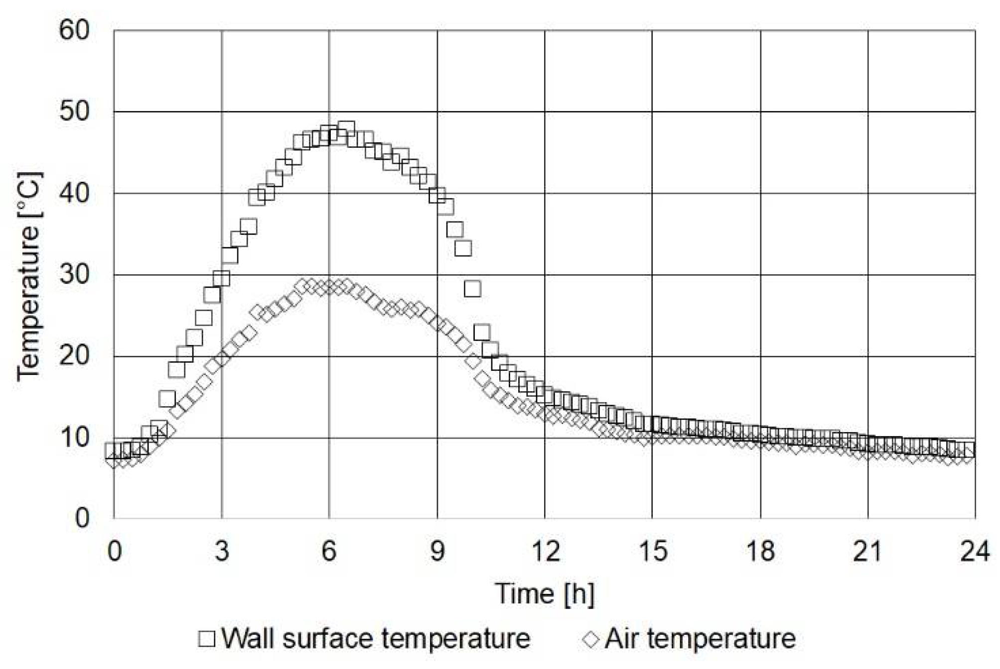
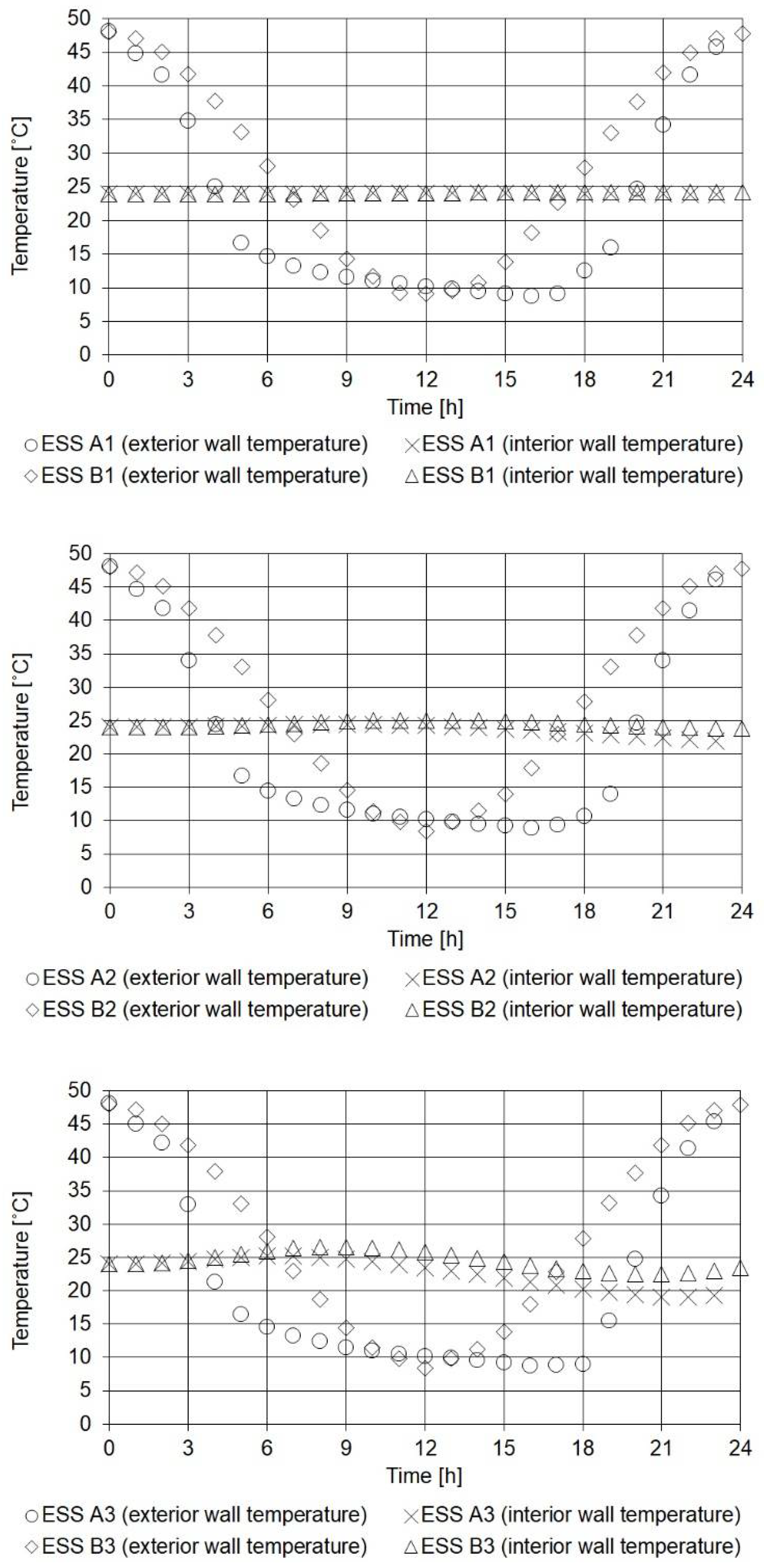
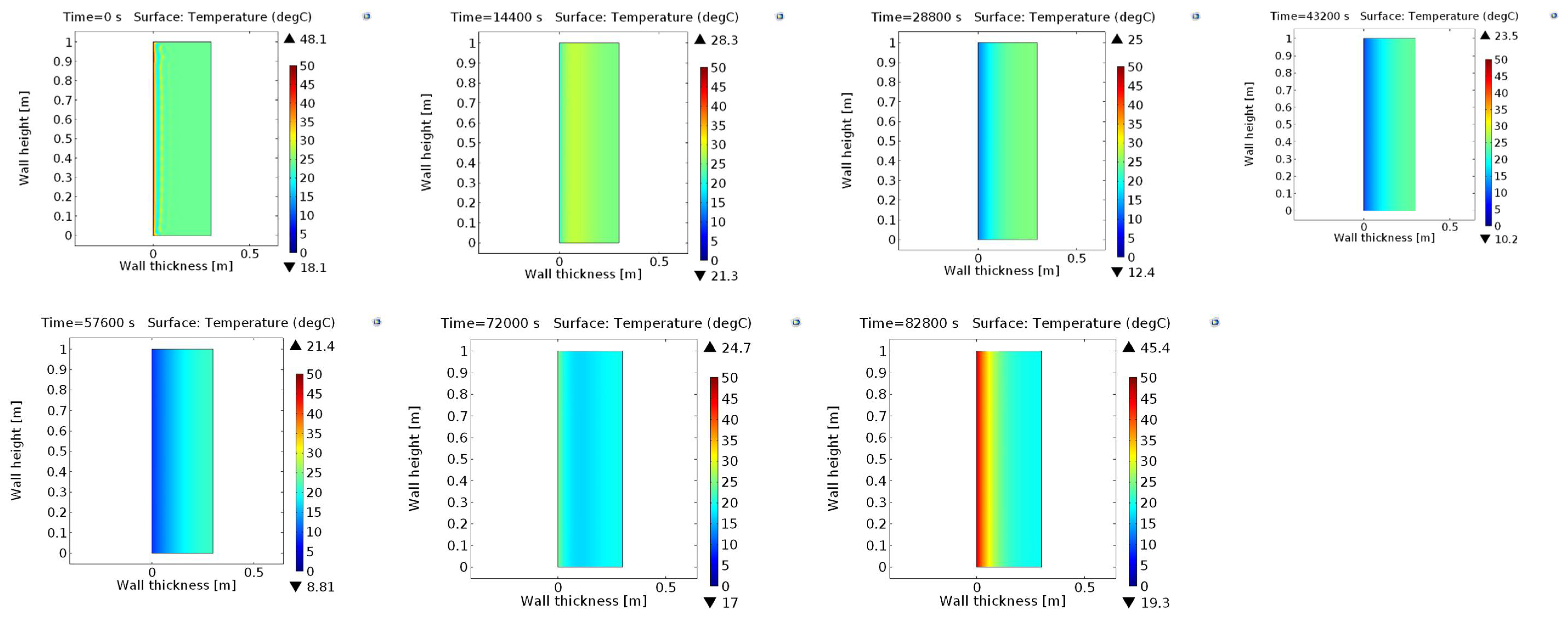
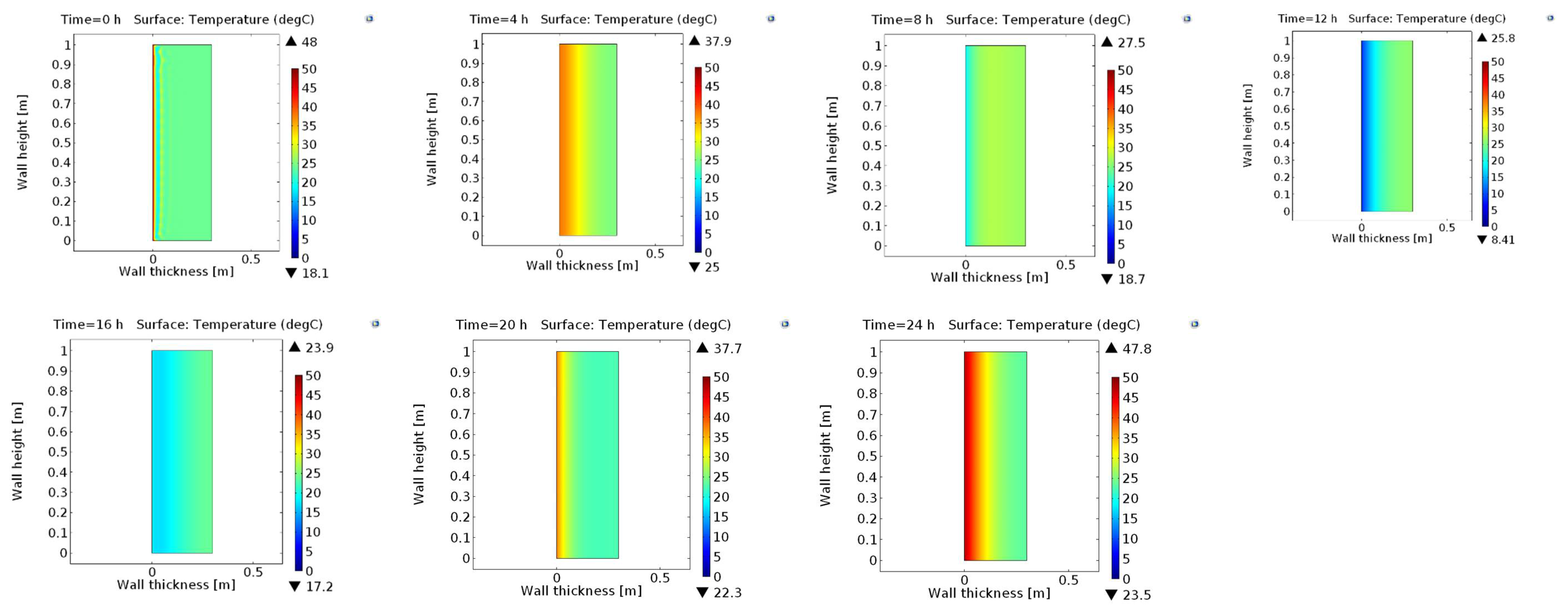
4.1. Exposed Wall in Sunny Spring Conditions (ESS)

Figure 2 demonstrates the effectiveness of the building walls of both Models A1 and B1 in maintaining the indoor wall temperatures at 24 °C. This is attributable to the low thermal conductivity of the wall’s construction material (k = 0.2 W/m² K), which allows for a very low value of heat flux―approximately 200 W/m², also verified by the data presented in

Table 3. Total heat flux of the building wall models under investigation and deviations.

Simulation Building Wall Model	Total Heat Flux, Q (W/m2)	Deviation of Model B from Model A (%)
ESS A1	206.91	-
ESS A2	529.34
ESS A3	1066.58
ESS B1	202.80	1.99
ESS B2	519.84	1.79
ESS B3	1074.97	0.79
NESS A1	125.53	-
NESS A2	310.50
NESS A3	603.57
NESS B1	127.68	1.71
NESS B2	325.84	4.94
NESS B3	675.68	11.95
ESW A1	175.17	-
ESW A2	418.36
ESW A3	766.07
ESW B1	146.70	16.25
ESW B2	368.77	11.86
ESW B3	716.78	6.43

. Evidently, the temperature profiles of Models A1 and B1 are in very good agreement.

Table 4. Building wall properties and boundary conditions of numerical simulation study for the building wall models under investigation.

Simulation Building Wall Model	Material Properties	Boundary Conditions
	Thermal Conductivity, k (W/m K)	Weather Conditions	Exterior Boundary Conditions, Text (°C)
ESS A1	0.2	ESS	24-h actual surface temperature data (see Appendix A)
ESS A2	0.5
ESS A3	1.0
ESS B1	0.2	ESS	28.05 + 19.75 sin [2π (t/24)]
ESS B2	0.5
ESS B3	1.0
NESS A1	0.2	NESS	24-h actual surface temperature data (see Appendix A)
NESS A2	0.5
NESS A3	1.0
NESS B1	0.2	NESS	23.58 + 12.67 sin [2π (t/24)]
NESS B2	0.5
NESS B3	1.0
ESW A1	0.2	ESW	24-h actual surface temperature data (see Appendix A)
ESW A2	0.5
ESW A3	1.0
ESW B1	0.2	ESW	17.62 + 12.98 sin [2π (t/24)]
ESW B2	0.5
ESW B3	1.0

indicates the detail of each investigated case study model. The simulation results of the models, considering the real surface temperature measurements for the external boundary conditions (Models A), are assessed against the respective model results employing the developed sinusoidal function (Models B). The temperature profiles of the exterior wall boundaries across all models, as expected, appear to be very similar since the exterior temperatures are not affected by the conductivity of the building wall. However, considerable deviation between the temperatures values of the pairs (Models A and B) is observed.

4.2. Exposed Wall in Sunny Spring Conditions (ESS)

Figure 2 demonstrates the effectiveness of the building walls of both Models A1 and B1 in maintaining the indoor wall temperatures at 24 °C. This is attributable to the low thermal conductivity of the wall’s construction material (k = 0.2 W/m² K), which allows for a very low value of heat flux―approximately 200 W/m², also verified by the data presented in Table 3. Evidently, the temperature profiles of Models A1 and B1 are in very good agreement.

With reference to Models A2 and B2, the interior wall temperatures appear to fluctuate between 22 °C and 25 °C over a period of 24 h. The reasoning behind this is the higher thermal conductivity of the building material (k = 0.5 W/m² K); in fact, the total average heat fluxes of two models for a 24 h period were estimated to be around 500 W/m² (Table 3). The temperature profiles of Models A2 and B2 reveal minor deviations in the results. More specifically, Model A2, which considers the real surface temperature measurements for the external boundary conditions, indicates a gradual drop of the temperature of the interior wall boundary during the period of midnight to midday, dropping to 22 °C. Model B2 simulates a small rise in the temperature of the interior wall boundary during the night time, reaching 25 °C, as a result of the external environmental conditions during the daytime. The small peak is followed by the restoration of the initial indoor temperature, as shown in Figure 2.

The indoor wall temperature profiles for Models A3 and B3 indicate considerable temperature fluctuations, as well as significant deviations between the two. The indoor wall temperature for Model A3 fluctuates between 25 °C at night and 19 °C in the morning, while for Model B3 it fluctuates between 26.5 °C and 22.5 °C. It is noteworthy that the indoor wall temperature for Model B3 is restored by hour 24, while this is not the case for Model A3. These differences are also evident in the 2D temperature contours, illustrated in Figure 3 and Figure 4 for a time period of 24 h with four (4) hour time steps. Figure 3 presents the temperature contours of the model using 24 h actual surface temperature data for the modelling of the external boundary conditions, while Figure 4 represents the model whose external boundary conditions are defined by the sinusoidal function of the EN ISO 13786:2007. The temperature fluctuations in the indoor temperature are a result of the increased U-value of the building wall; in fact the total average heat fluxes of the two models for a 24 h period exceed 1000 W/m² (Table 3).

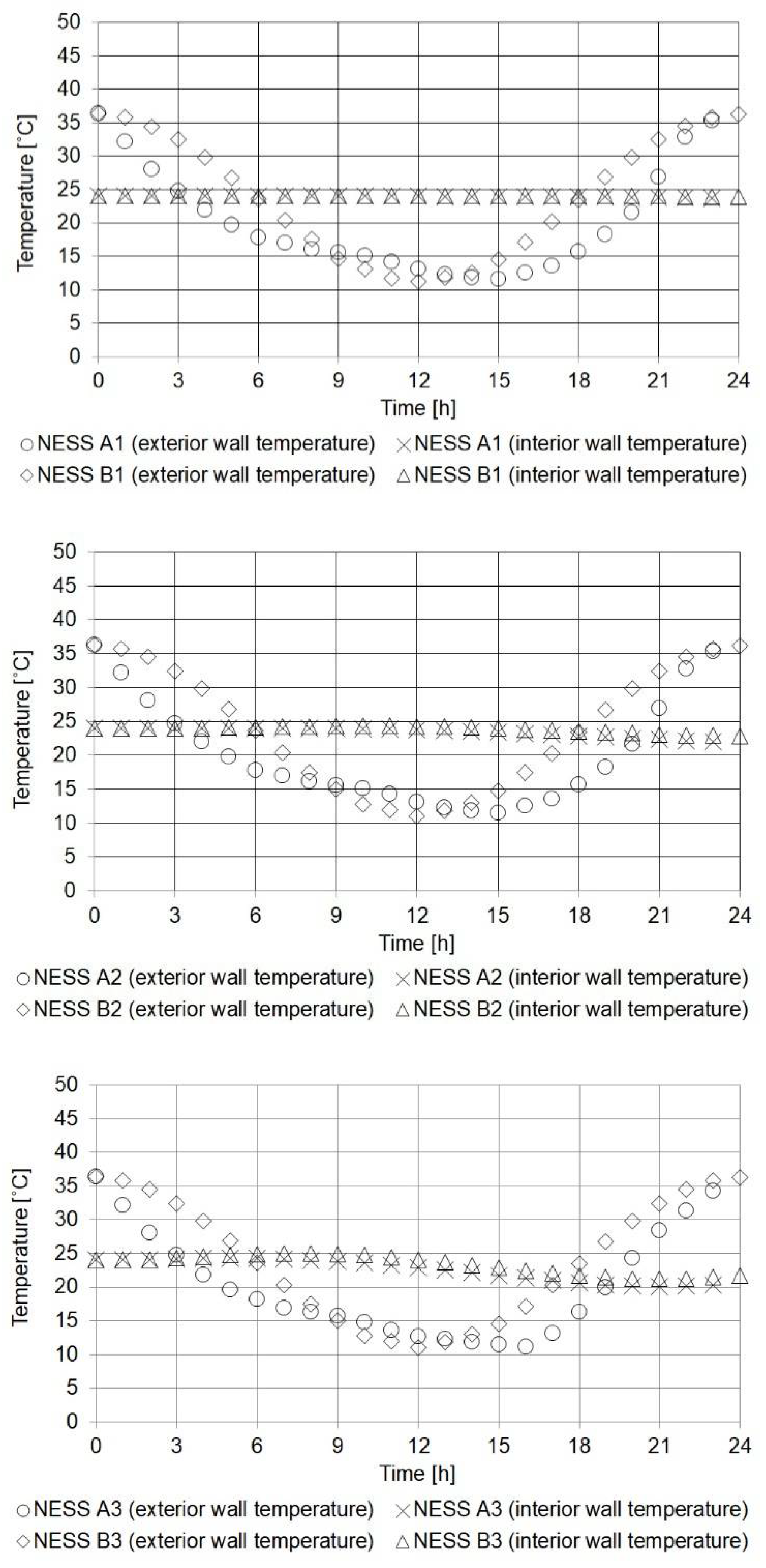
4.3. Non-Exposed Wall in Sunny Spring Conditions (NESS)

Similarly to the previous case, the indoor wall temperature for Models A1 and B1 are maintained at 24 °C throughout the day (Figure 5). With reference to Models A2, B2, A3, and B3, the interior temperatures are noted to be more susceptible to the exterior fluctuating conditions, reaching as low as 20 °C in Model A3. Furthermore, the temperature profiles comparing Models A2 and B2, and Models A3 and B3 reveal smaller deviations in the results to the ESS case. Noteworthy is the fact that the difference in the indoor temperatures of Models A3 and B3 has decreased to 1.2 °C from 2.5 °C in the ESS case.

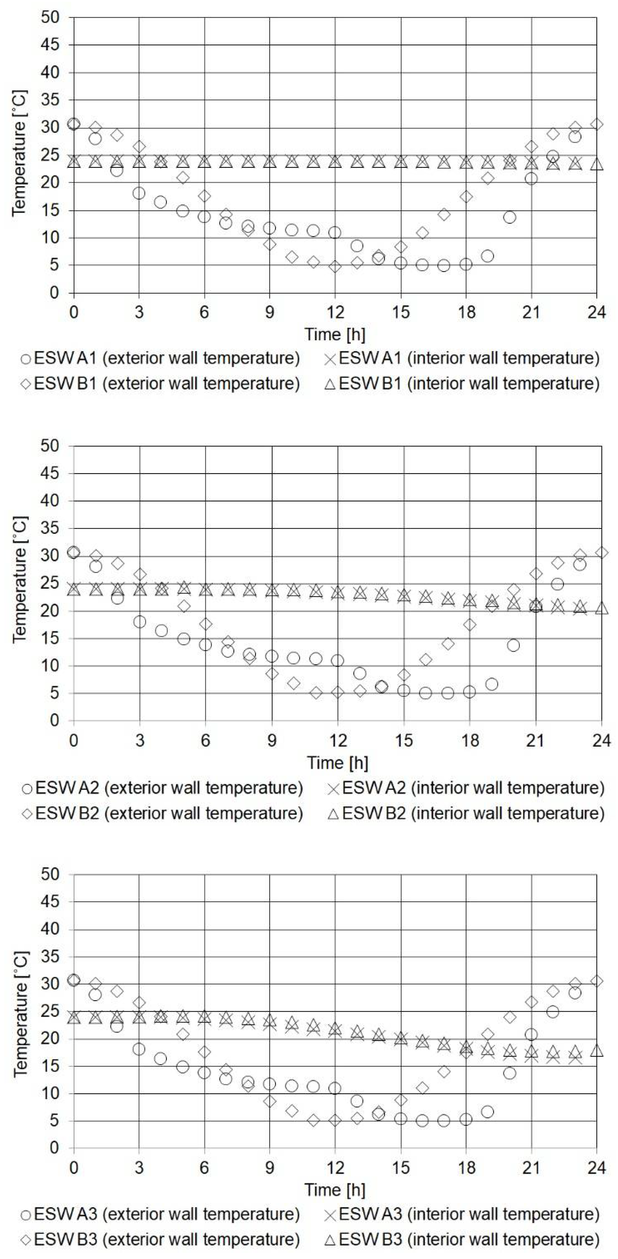
4.4. Exposed Wall in Sunny Winter Conditions (ESW)

For the case of an exposed wall in sunny winter conditions, a similar pattern is indicated; the indoor temperatures for the case of the wall with the lowest thermal conductivity are unaffected by the external conditions (Figure 6). On the other hand, the indoor wall temperatures have dropped by 3 °C and 7 °C in the models with building walls of 0.5 W/m² K and 1.0 W/m² K thermal conductivity, respectively. However, the interior temperature profiles for Models A and B across all three cases

4.5. Heat Flux of Building Walls Under Investigation

In order to establish quantitatively whether the sinusoidal function defined by the EN ISO 13786:2007 for the modelling of the external boundary conditions provides a reliable representation of the actual weather conditions that building walls experience, the total heat fluxes for the models under investigation for a 24 h period were calculated using data obtained from the employed numerical simulation tool and these are provided in Table 3. With reference to the ESS condition, Models B show very small deviations from their respective Models A, at less than 2% for each case study. On the contrary, the deviations of the heat fluxes for the NESS and ESW conditions are greater. In the NESS case, the deviation of Model B3 from Model A3 reaches 12%, while for the case of ESW, Model B1 deviates from its respective Model A1 by 16%. The results indicate that the sinusoidal function defined by the relevant standards for the modelling of the external boundary conditions is accurate for the case of an exposed wall in sunny spring conditions, whereas quite considerable differences are noted for the cases of a non-exposed walls in sunny spring conditions and of exposed walls in sunny winter conditions.

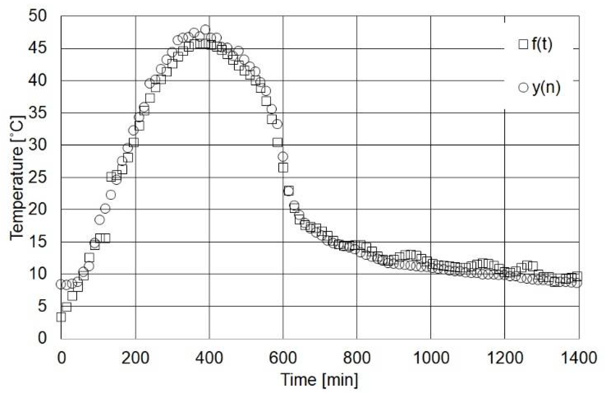
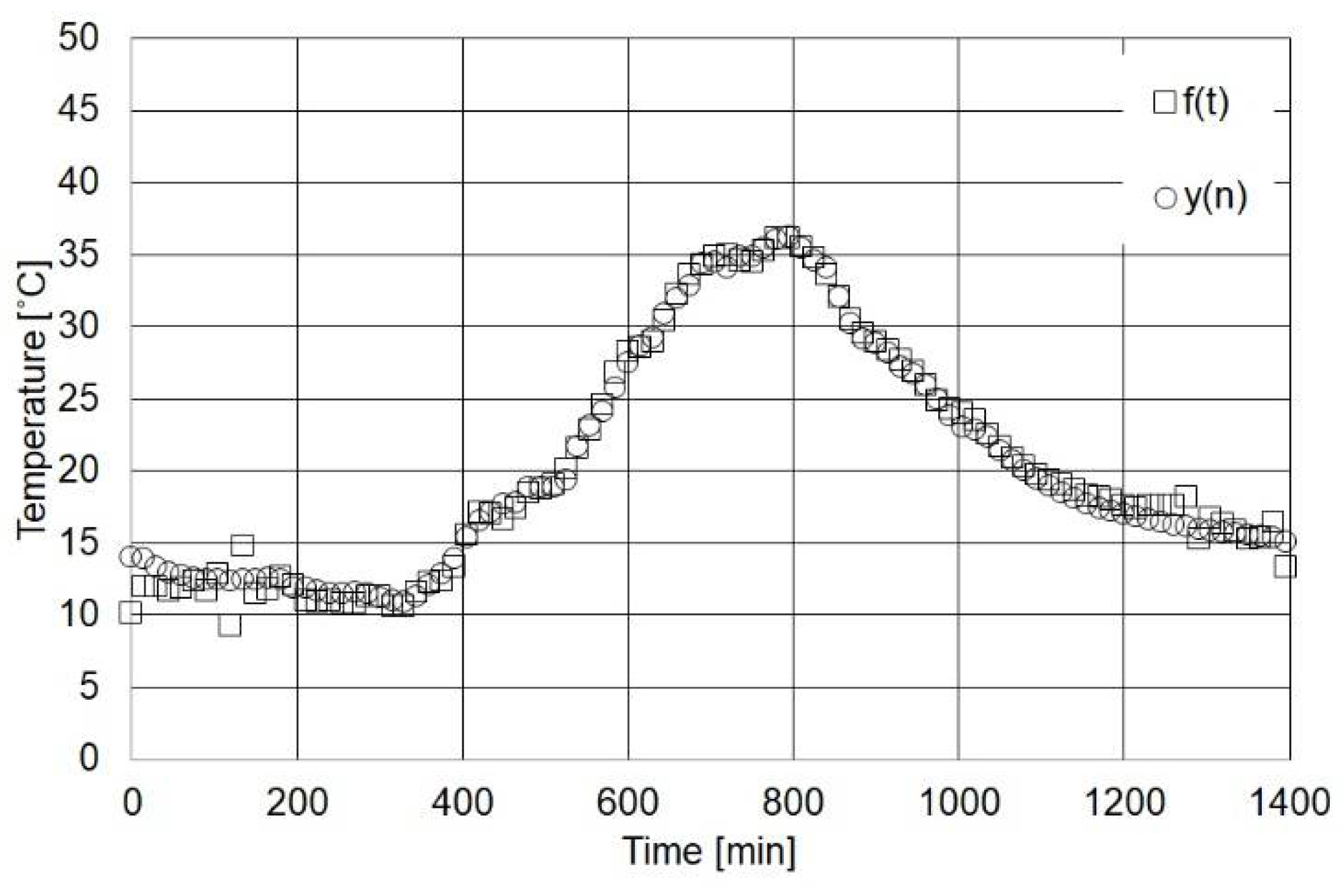
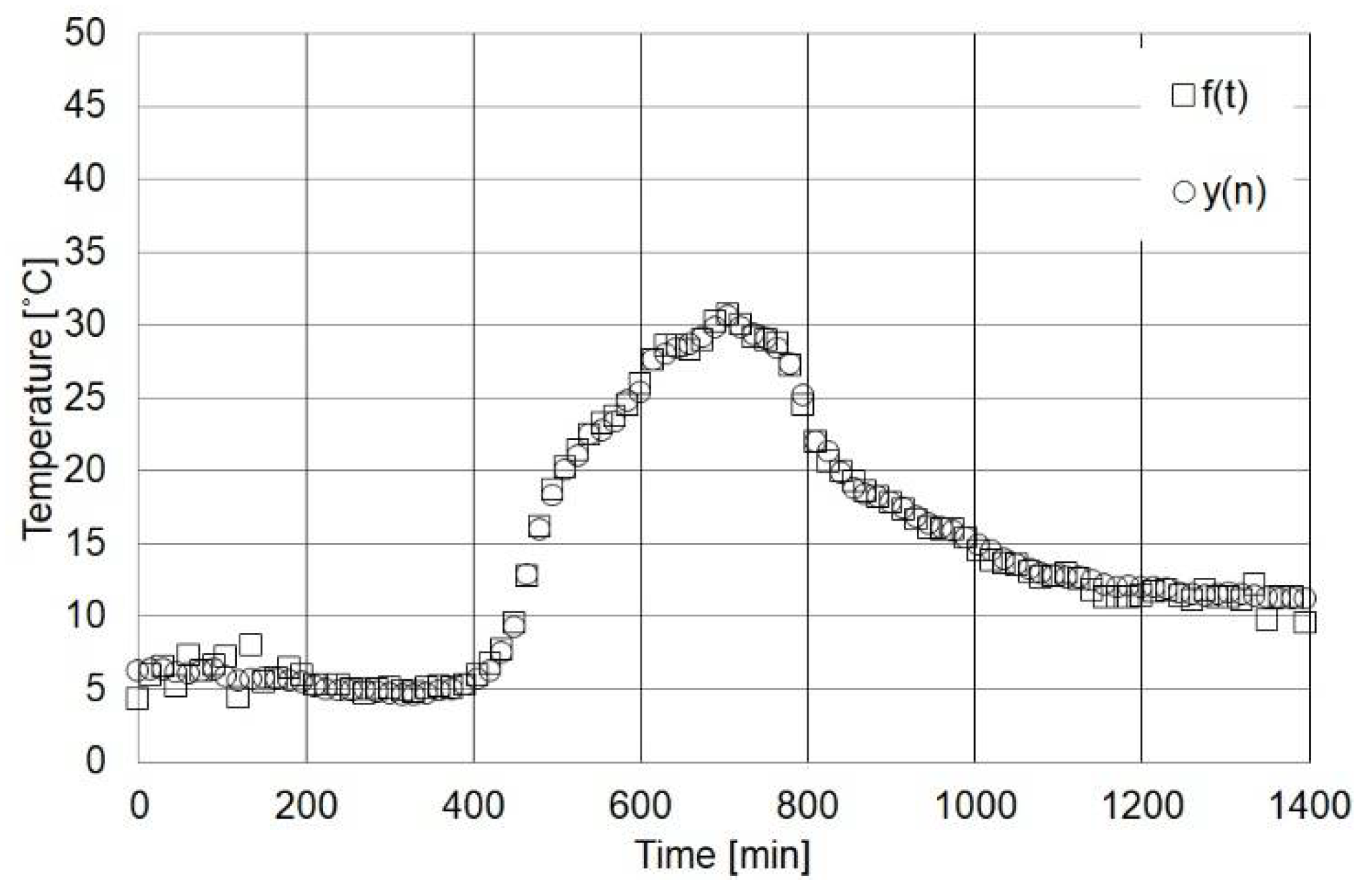
5. Function Modeling from Measured Data

For the reliable simulation of the actual weather conditions that the walls of buildings are experiencing, this study introduces a signal reconstruction algorithm, presented in Table 2. This algorithm follows a novel approach by reconstructing the actual temperature versus time signal for the simulation of the actual boundary conditions. The measured data over a 24 h period are represented as a vector, $y\left(n\right)$, and are modelled using a continuous time function comprised of a sum of the amplitude scaled, time-shifted, frequency shifted, and time scaled waveforms, as defined in Section 3 of this work. Accordingly, the settings of the signal reconstruction algorithm are the following:

$${\tau }_{min}=0 \mathrm{s},{\tau }_{step}=900 \mathrm{s},{\tau }_{max}=9000 \mathrm{s}$$

$$v_{min}=0,v_{step}=5.56\times {10}^{-7},v_{max}=1.11\times {10}^{-4}$$

$$a_{min}={10}^7,a_{step}=100,a_{max}={10}^8$$

$$T=1440 \min ,T^{\prime }=1290 \min ,J=50,T_S=15 \min ,N=96.$$

The comparison between the actual measured temperature data points, represented by the vector $y\left(n\right)$, and the continuous function, $f\left(t\right)$, provided by the signal re-construction algorithm for:

• an exposed wall in sunny spring conditions (ESS);
• a non-exposed wall in sunny spring conditions (NESS); and
• an exposed wall in sunny winter conditions (ESW)

are provided in Figure 7, Figure 8 and Figure 9, respectively.

6. Conclusions

External boundary conditions play a crucial role in the investigation of the thermal performance of building elements using finite element numerical simulation. ISO 13786:2007 indicates that these conditions can be represented by a sinusoidal function with time, which is a simplified approach followed in numerous scientific studies in the literature but is, however, inaccurate. The key objectives of this work were to investigate the accuracy of numerical simulation results for the thermal performance of building elements generated by adopting the sinusoidal temperature boundary condition assumption, and to propose an improved model for the definition of the external boundary conditions. In this context, numerical simulation models for different case studies that employed 24 h actual surface temperature data and the sinusoidal temperature boundary conditions were developed. The results of this analysis indicated that the sinusoidal function does not correctly represent the actual thermal performance of building elements, with deviations of up to 16% in terms of total heat fluxes. On the contrary, the proposed signal reconstruction algorithm achieves the accurate simulation of the actual boundary conditions by accurately describing the variation of the actual temperature versus time. Accordingly, the algorithm establishes a novel approach in computational building physics in regard to the boundary conditions of simulated building elements, which will enable a more precise modelling of building performance for the transition of the European building stock [16].

References

1. 13790:2008. Energy Performance of Buildings—Calculation of Energy Use for Space Heating and Cooling; ISO: Geneva, Switzerland, 2008.
2. Fokaides, P.A.; Maxoulis, C.N.; Panayiotou, G.P.; Neophytou, M.K.A.; Kalogirou, S.A. Comparison between measured and calculated energy performance for dwellings in a summer dominant environment. Energy Build. 2011, 43, 3099–3105. [Google Scholar] [CrossRef]
3. Kylili, A.; Fokaides, P.A. Numerical simulation of phase change materials for building applications: A review. Adv. Build. Energy Res. 2015, 11, 1–25. [Google Scholar] [CrossRef]
4. 13786:2007. Thermal Performance of Building Components—Dynamic Thermal Characteristics—Calculation Methods; ISO: Geneva, Switzerland, 2007.
5. Kontoleon, K.J.; Eumorfopoulou, E.A. The influence of wall orientation and exterior surface solar absorptivity on time lag and decrement factor in the Greek region. Renew. Energy 2008, 33, 1652–1664. [Google Scholar] [CrossRef]
6. Zhang, Z.L.; Wachenfeldt, B.J. Numerical study on the heat storing capacity of concrete walls with air cavities. Energy Build. 2009, 41, 769–773. [Google Scholar] [CrossRef]
7. Viot, H.; Sempey, A.; Pauly, M.; Mora, L. Comparison of different methods for calculating thermal bridges: Application to wood-frame buildings. Build. Environ. 2015, 93, 339–348. [Google Scholar] [CrossRef]
8. Yang, J.; Yu, J.; Xiong, C. Heat Transfer Analysis of Hollow Block Ventilated Wall Based on CFD Modeling. Procedia Eng. 2015, 121, 1312–1317. [Google Scholar] [CrossRef]
9. Tariku, F.; Kumaran, K.; Fazio, P. Integrated analysis of whole building heat, air and moisture transfer. Int. J. Heat Mass Transf. 2010, 53, 3111–3120. [Google Scholar] [CrossRef] [Green Version]
10. Abahri, K.; Belarbi, R.; Trabelsi, A. Contribution to analytical and numerical study of combined heat and moisture transfers in porous building materials. Build. Environ. 2011, 46, 1354–1360. [Google Scholar] [CrossRef]
11. Kontoleon, K.J. Dynamic thermal circuit modelling with distribution of internal solar radiation on varying façade orientations. Energy Build. 2012, 47, 139–150. [Google Scholar] [CrossRef]
12. Liu, X.; Chen, Y.; Ge, H.; Fazio, P.; Chen, G.; Guo, X. Determination of optimum insulation thickness for building walls with moisture transfer in hot summer and cold winter zone of China. Energy Build. 2015, 109, 361–368. [Google Scholar] [CrossRef]
13. Mazzeo, D.; Oliveti, G.; Arcuri, N. Multiple Bi-phase Interfaces in a PCM Layer Subject to Periodic Boundary Conditions Characteristic of Building External Walls. Energy Procedia 2015, 82, 472–479. [Google Scholar] [CrossRef]
14. Fokaides, P.A.; Christoforou, E.A.; Kalogirou, S.A. Legislation driven scenarios based on recent construction advancements towards the achievement of nearly zero energy dwellings in the southern European country of Cyprus. Energy 2014, 66, 588–597. [Google Scholar] [CrossRef]
15. Mallat, S.G.; Zhang, Z. Matching pursuits with time-frequency dictionaries. IEEE Trans. Signal Process. 1993, 41, 3397–3415. [Google Scholar] [CrossRef] [Green Version]
16. Kylili, A.; Fokaides, P.A. European smart cities: The role of zero energy buildings. Sustain. Cities Soc. 2015, 15, 86–95. [Google Scholar] [CrossRef]
Figure 1. Wall surface and air temperatures for an exposed vertical building element.
Energies 11 01520 g001
Figure 2. Simulation results for building wall models A and B for sunny spring conditions (ESS).
Energies 11 01520 g002
Figure 3. Two-dimensional (2D) temperature contours for a time period of 24 h (time step: 4 h) for the exposed wall of thermal conductivity of 1 W/m K in sunny spring conditions (SSE), using 24-h actual surface temperature data for the modeling of the external boundary conditions. Note: left-hand boundary of the model: exterior wall surface; right-hand boundary of model: interior wall surface.
Energies 11 01520 g003
Figure 4. Two-dimensional (2D) temperature contours for a time period of 24 h (time step: 4 h) for the exposed wall of thermal conductivity of 1 W/m K in sunny spring conditions (SSE), using the sinusoidal function defined by the EN ISO 13786:2007 for the modeling of the external boundary conditions. Note: left-hand boundary of model: exterior wall surface; right-hand boundary of model: interior wall surface.
Energies 11 01520 g004
Figure 5. Simulation results for building wall models A and B for non-exposed wall in sunny spring conditions (NESS).
Energies 11 01520 g005
Figure 6. Simulation results for building wall models A and B for sunny winter conditions (ESW).
Energies 11 01520 g006
Figure 7. Measured temperature data points versus the continuous function provided by the signal reconstruction algorithm for an exposed wall in sunny spring conditions (ESS).
Energies 11 01520 g007
Figure 8. Measured temperature data points versus the continuous function provided by the signal reconstruction algorithm for a non-exposed wall in sunny spring conditions (NESS).
Energies 11 01520 g008
Figure 9. Measured temperature data points versus the continuous function provided by the signal reconstruction algorithm for an exposed wall in sunny winter conditions (ESW).
Energies 11 01520 g009