Artificial Neural Network–Based Control of a Variable Refrigerant Flow System in the Cooling Season


Abstract
:1. Introduction
2. ANN Model for Predicting Cooling Energy of the VRF System
2.1. ANN Literature Review on Building Thermal Controls
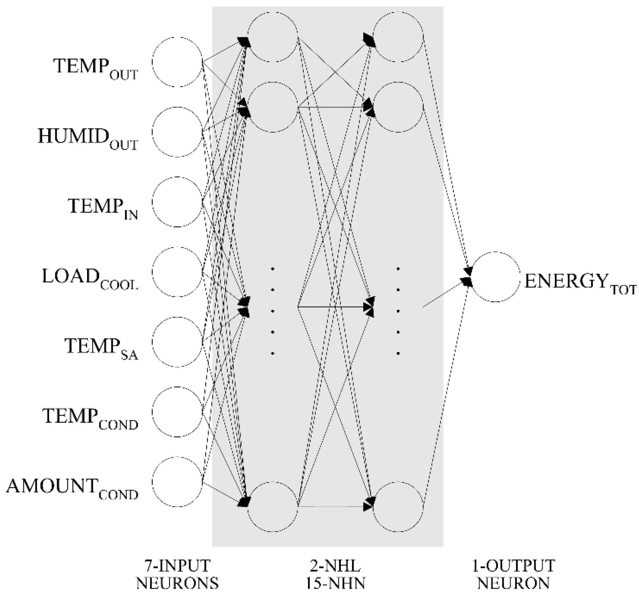
2.2. Development Process of the Predictive Model
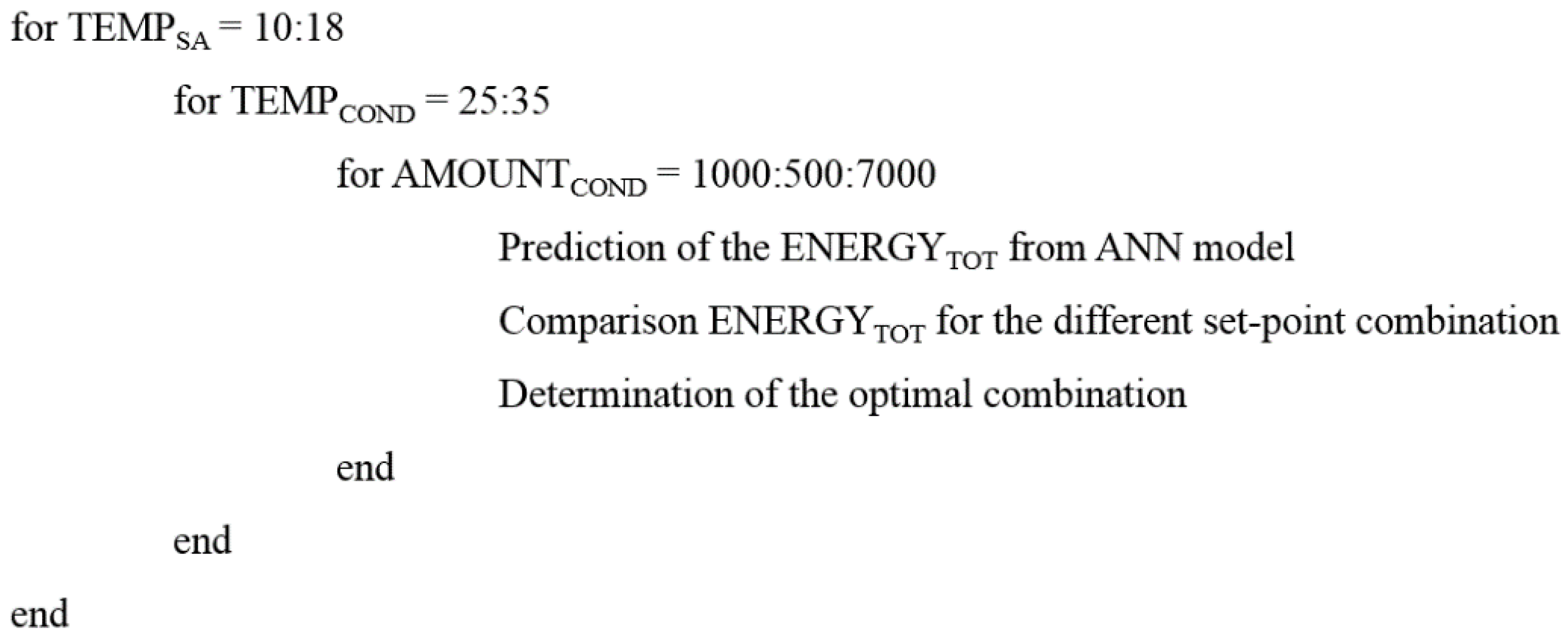
3. Development and Evaluation of the Predictive Control Algorithm
4. Performance of the Predictive Control Algorithm
5. Conclusions
- (1)
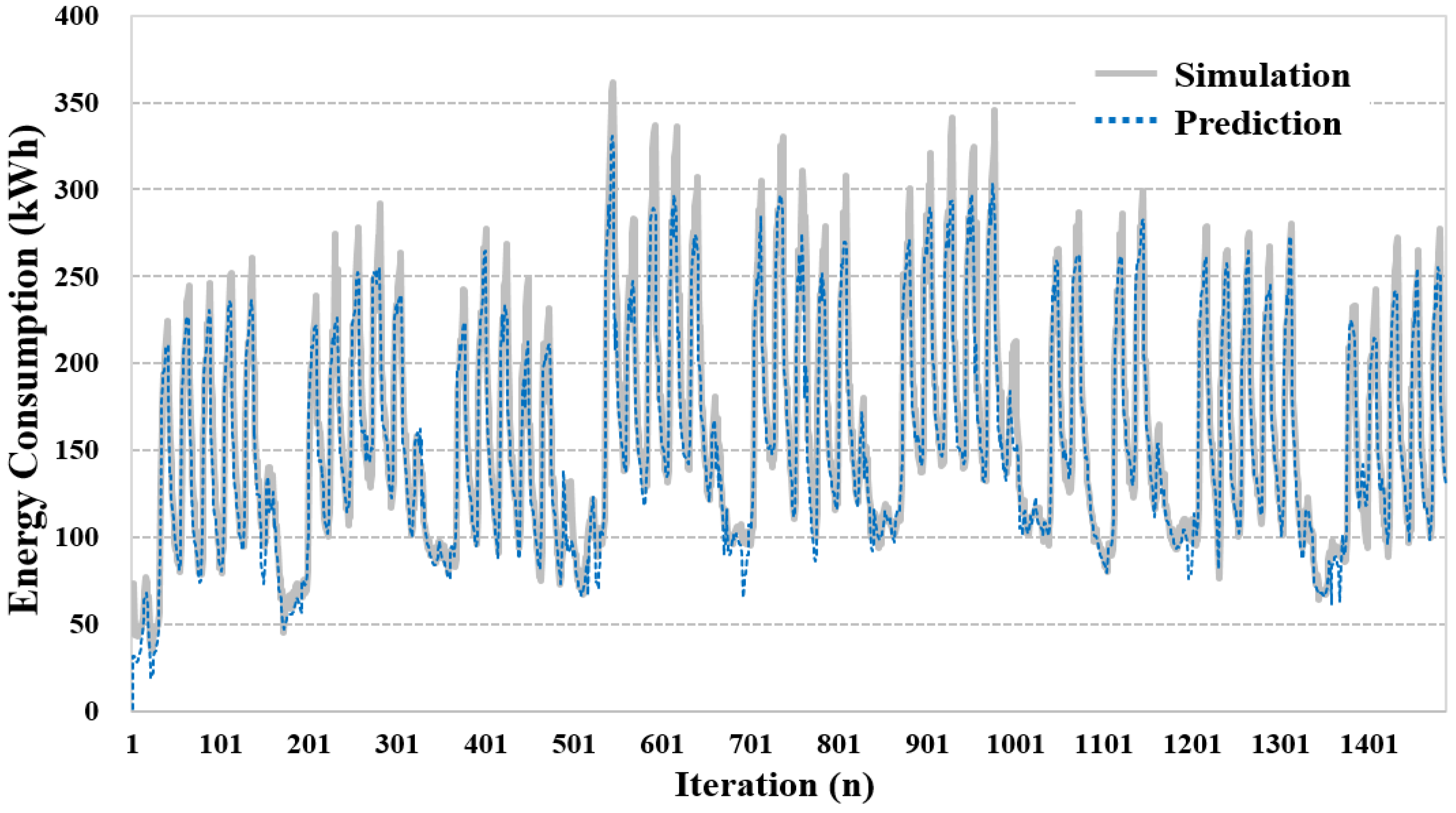
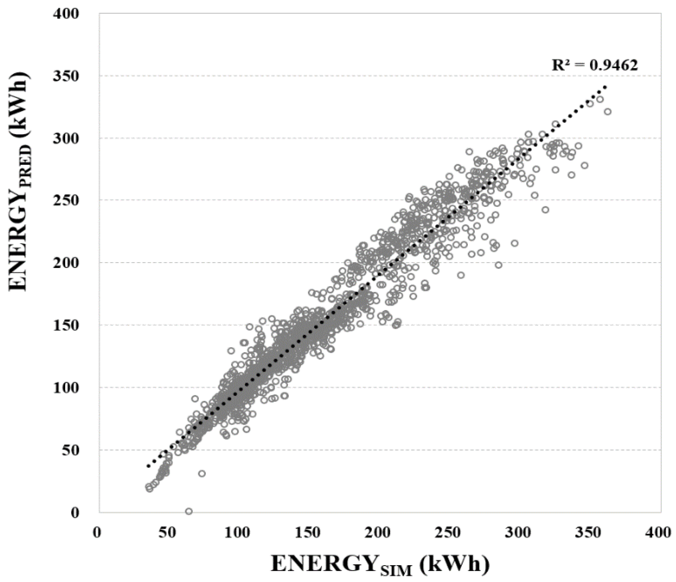
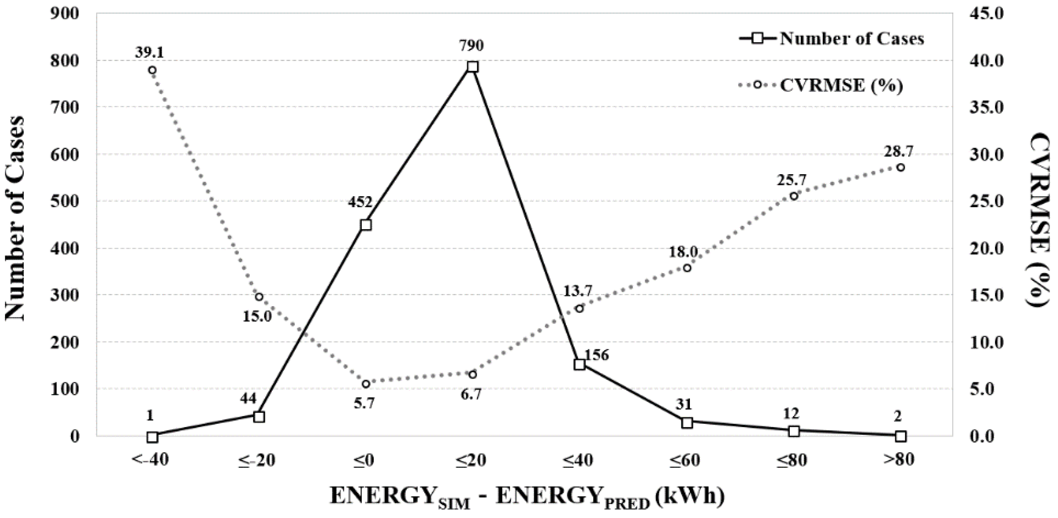
- The prediction model embedded in the control algorithm showed an acceptable prediction accuracy. For the number of cycles (1488 h), the results revealed the CVRMSE of 10.3% between the simulated and predicted cooling energy.
- (2)
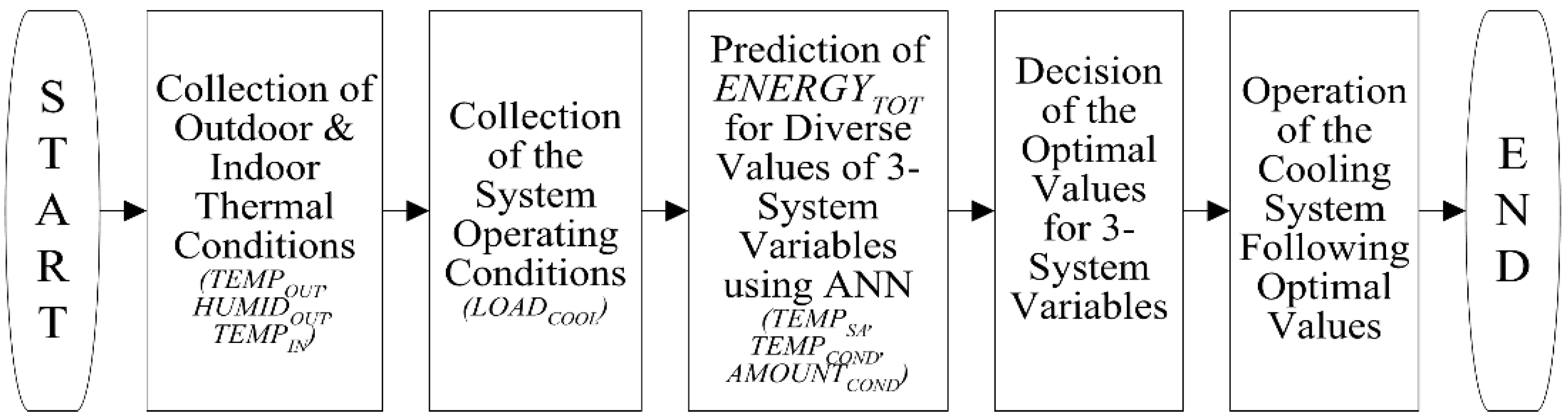
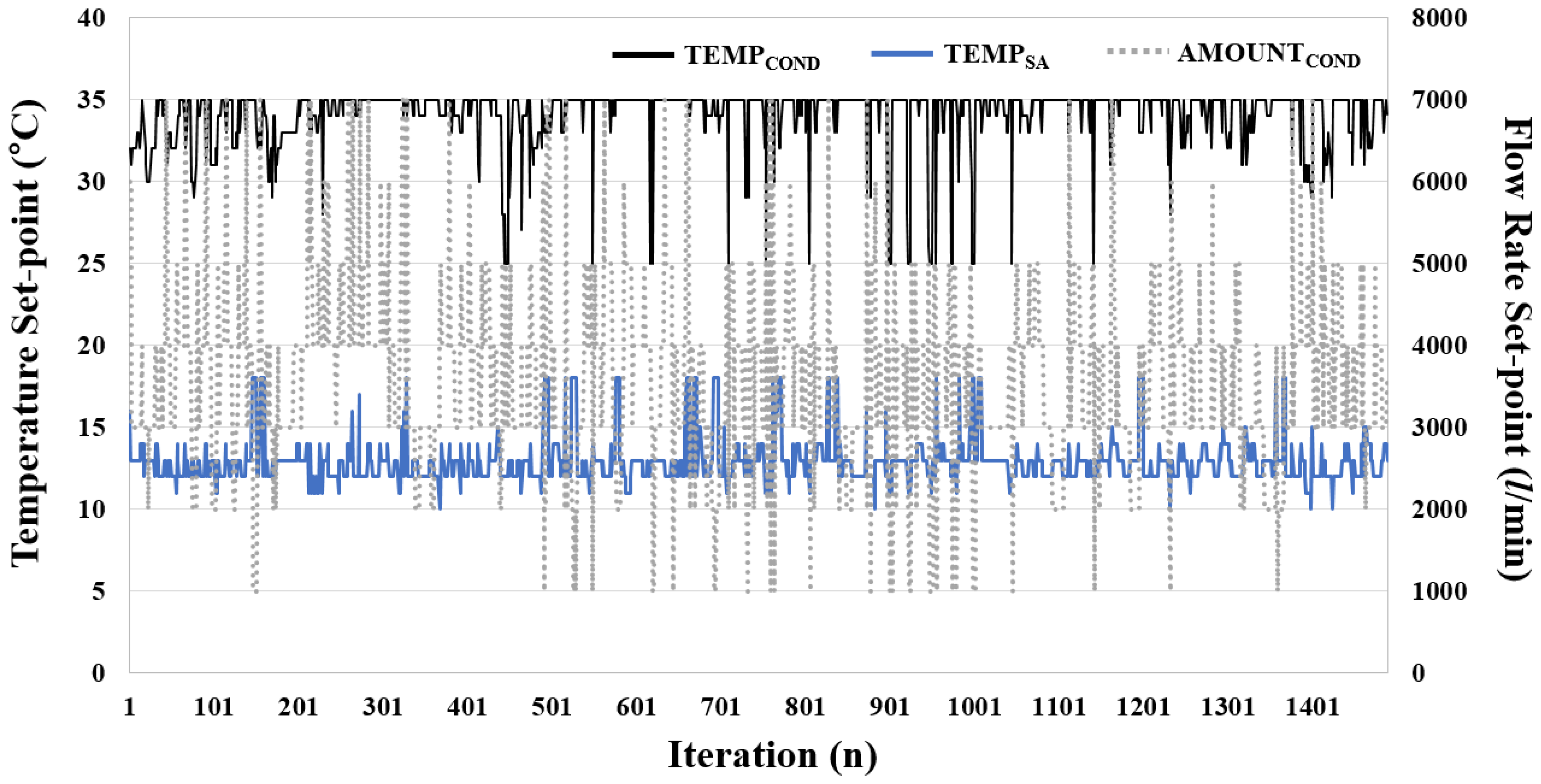
- The ANN-based predictive control algorithm determined the optimal set-points of the VRF system. For most of the cases, TEMPSA, TEMPCOND, and AMOUNTCOND were in the stable range of 12–14 °C, 35 °C, and 3000–5000 L/min, respectively
- (3)
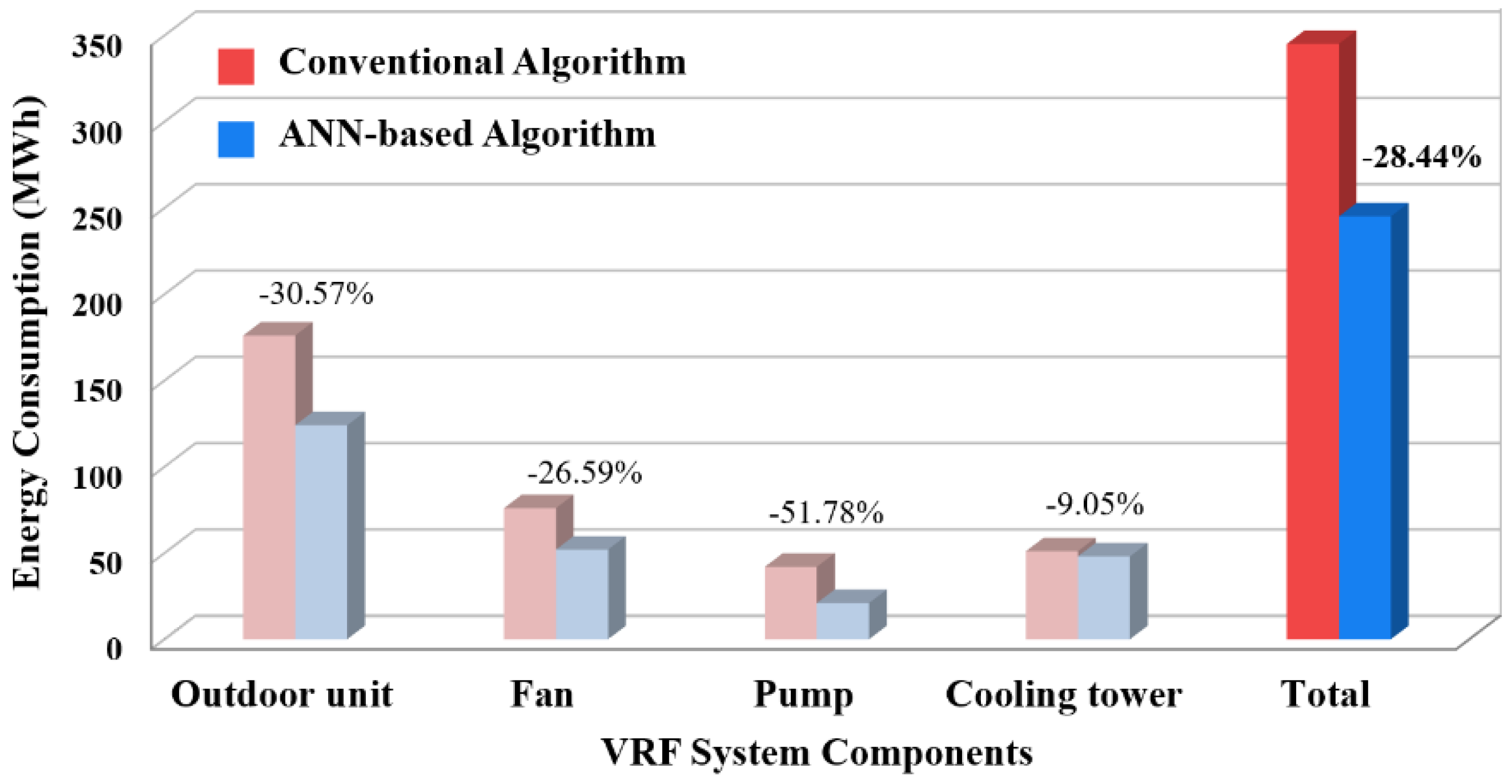
- The algorithm also markedly saved the cooling energy consumption of the VRF cooling system during the 62 days from the 1 July to the 31 August. The total cooling energy saved was 28.44%, which corresponds to an electrical energy reduction of approximately 95,509 kWh or 13,562,278 Korean won (12,054 U.S. dollars).
Author Contributions
Funding
Acknowledgments
Conflicts of Interest
Nomenclature
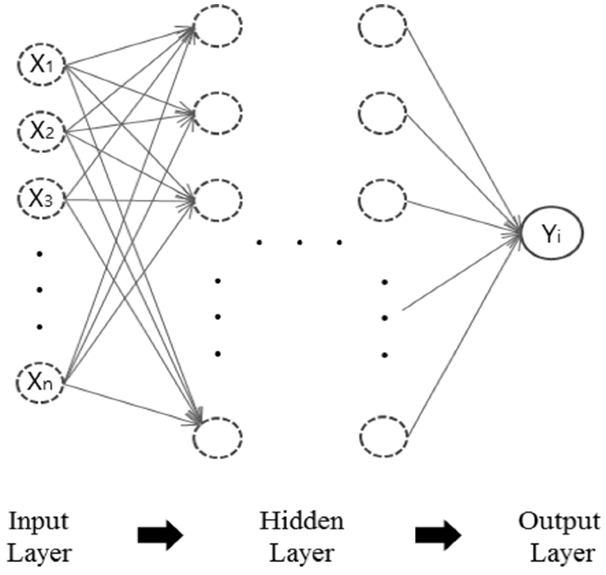
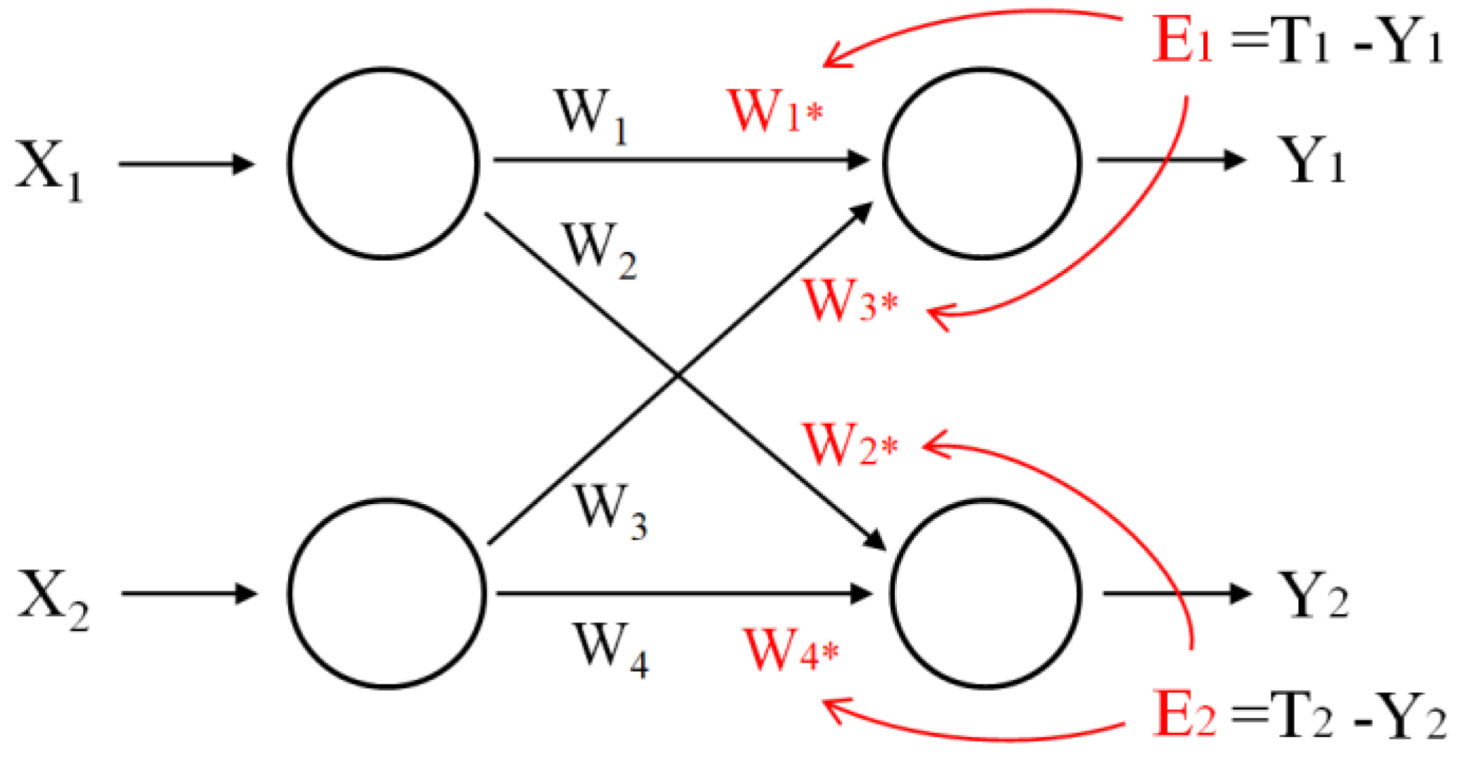
| ANN | artificial neural network |
| OECD | organization for economic cooperation and development |
| TOE | ton of oil equivalent |
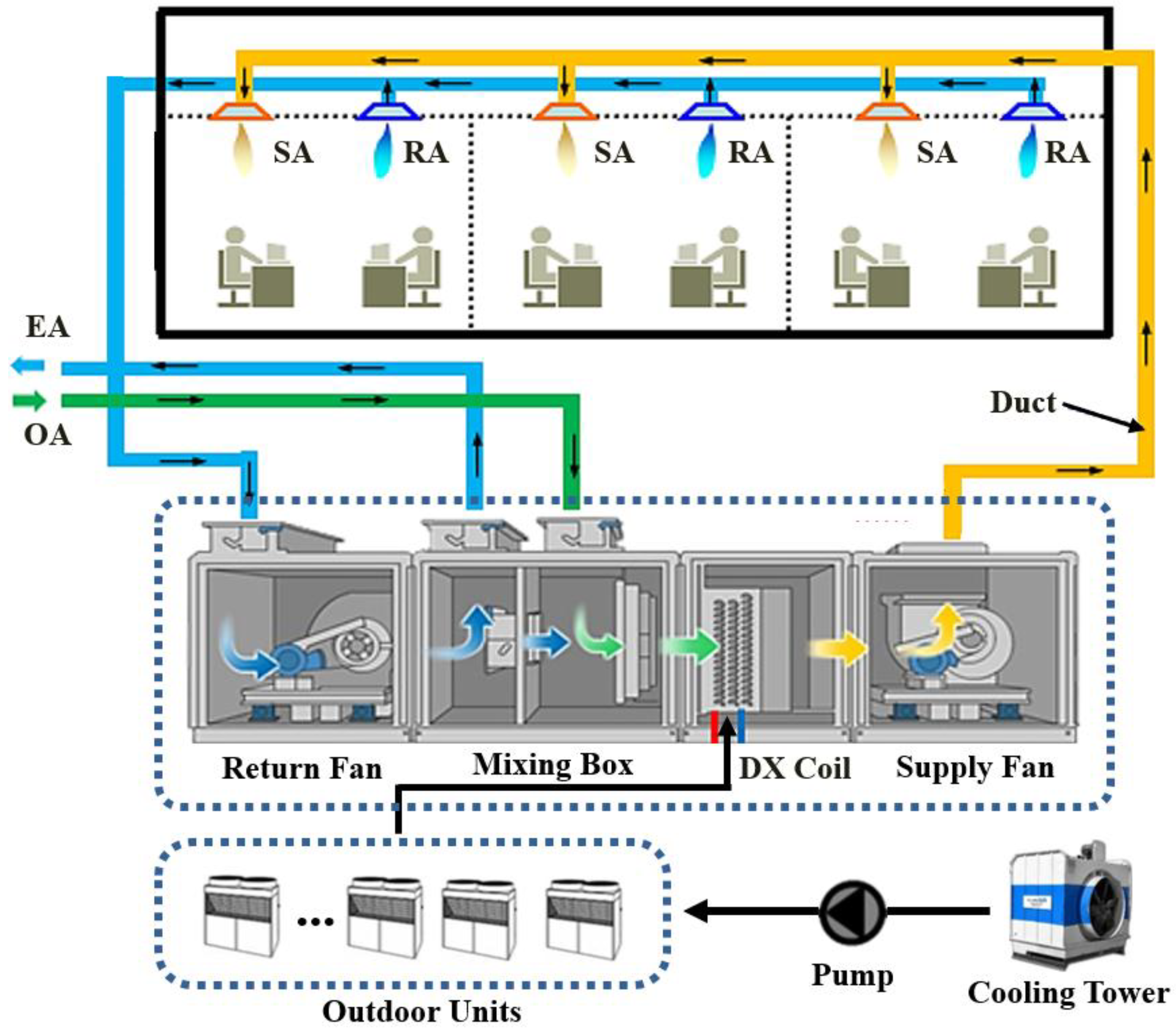
| DX AHU | direct expansion air handling unit |
| R2 | coefficient of determination |
| CVRMSE | coefficient of variation root mean square error |
| ASHRAE | American Society of Heating, Refrigerating and Air-Conditioning Engineers |
| SA | supply air |
| RA | return air |
| EA | exhaust air |
| OA | outdoor air |
| TEMPSA | air handling unit supply air temperature set-point (°C) |
| TEMPCOND | condenser fluid temperature set-point (°C) |
| AMOUNTCOND | condensing warm fluid amount set-point (liter/minute) |
| TEMPOUT | average outdoor temperature (°C) |
| HUMIDOUT | average outdoor humidity (%) |
| SOLAR | average solar radiation (W/m2) |
| TEMPIN | average indoor temperature (°C) |
| LOADCOOL | internal load that generated from the cooling tower (kWh) |
| ENERGYTOT | predicted total cooling energy for the next 1 h (kWh) |
| NHL | number of hidden layer |
| NHN | number of hidden neuron in each hidden layer |
| LR | learning rate |
| MO | moment |
References
- Meehl, G.A.; Tebaldi, C. More intense, more frequent, and longer lasting heatwaves in the 21st Century. Science 2004, 305, 994–997. [Google Scholar] [CrossRef] [PubMed]
- International Energy Agency. Energy Balances of OECD/Non-OECD Countries; IEA Statistics: Paris, France, 2015. [Google Scholar]
- Korea Energy Agency. 2016 Korea Energy Handbook; KEA: Yongin-si, Korea, 2016. [Google Scholar]
- Ahn, B.L.; Kim, C.H.; Kim, J.Y.; Jang, C.Y. A study on the analysis of building energy rating considering the region. J. Korean Sol. Energy Soc. 2009, 29, 53–58. [Google Scholar]
- Jang, H.I.; Cho, Y.H.; Jo, J.H. Application and improvement of the renewable energy management system in existing buildings. J. Architect. Inst. Korea 2013, 29, 227–234. [Google Scholar]
- Korea Energy Economics Institute. 2014 Energy Consumer Survey; Korea Energy Economics Institute: Ulsan, Korea, 2015. [Google Scholar]
- National Institute of Environmental Research. Greenhouse Gas Reduction Technologies and Their Costs in Commercial and Public Sector; National Institute of Environmental Research: Tsukuba, Japan, 2010. [Google Scholar]
- Korea Energy Economics Institute. Building Energy Consumption Standing Sampling Survey; Korea Energy Economics Institute: Ulsan, Korea, 2016. [Google Scholar]
- Korea Energy Agency. 2015 Energy Usage Statistics; KEA: Yongin-si, Korea, 2016. [Google Scholar]
- Ministry of Land, Infrastructure and Transport. The 1st Green Building Basic Plan; Ministry of Land, Infrastructure and Transport: Sejong, Korea, 2014. [Google Scholar]
- Lee, J.H.; Song, Y.H.; Yoon, H.J.; Choi, D.S.; Tae, S.J.; Kim, I.K. A study on development and effectiveness verification of set-point control algorithm for water-cooled VRF System. Soc. Air-Cond. Refrig. Eng. Korea 2016, 399–402. [Google Scholar]
- Aynur, T.N. Va riable refrigerant flow systems: A review. Energy Build. 2010, 42, 1106–1112. [Google Scholar] [CrossRef]
- Thornton, B.; Wagner, A. Variable Refrigerant Flow Systems; Pacific Northwest National Laboratory: Richland, WA, USA, 2012. [Google Scholar]
- Lee, K.H. A calculation method of the cooling performance for the direct expansion (DX) air handling unit (AHU)-water source VRF system. Soc. Air-Cond. Refrig. Eng. Korea 2016, 45, 64–68. [Google Scholar]
- Zhang, D.; Zhang, X.; Liu, J. Experimental study of performance of digital variable multiple air conditioning system under part load conditions. Energy Build. 2011, 43, 1175–1178. [Google Scholar] [CrossRef]
- Chung, M.H.; Yang, Y.K.; Lee, K.H.; Lee, J.H.; Moon, J.W. Application of artificial neural networks for determining energy-efficient operating set-points of the VRF cooling system. Build. Environ. 2017, 125, 77–87. [Google Scholar] [CrossRef]
- Panja, P.; Velasco, R.; Pathak, M.; Deo, M. Application of artificial intelligence to forecast hydrocarbon production from shales. Petroleum 2018, 4, 75–89. [Google Scholar] [CrossRef]
- Gupta, A.K.; Kumar, P.; Sahoo, R.K.; Sahu, A.K.; Sarangi, S.K. Performance measurement of plate fin heat exchanger by exploration: ANN, ANFIS, GA, and SA. J. Comput. Des. Eng. 2017, 4, 60–68. [Google Scholar] [CrossRef]
- Ferdyn-Grygierek, J.; Grygierek, K. Multi-variable optimization of building thermal design using genetic algorithms. Energies 2017, 10, 1570. [Google Scholar] [CrossRef]
- Yang, J.; Rivard, H.; Zmeureanu, R. Building energy prediction with adaptive artificial neural networks. In Proceedings of the 9th International IBPSA Conference, Montréal, QC, Canada, 15–18 August 2005; pp. 1401–1408. [Google Scholar]
- McCulloch, W.S.; Pitts, W. A logical calculus of ideas immanent in nervous activity. Bull. Math. Biophys. 1943, 5, 115–133. [Google Scholar] [CrossRef]
- Basheer, I.D.; Hajmeer, M. Artificial neural networks: Fundamentals, computing, design, and application. J. Microbiol. Meth. 2000, 43, 3–31. [Google Scholar] [CrossRef]
- Nielsen, F. Neural Networks-Algorithms and Application; Niels Brock Business College: København, Denmark, 2001. [Google Scholar]
- Zhang, G.; Patuwo, B.E.; Hu, M.Y. Forecasting with artificial neural networks: The state of the art. Int. J. Forecast. 1998, 14, 35–62. [Google Scholar] [CrossRef]
- Renno, C.; Petito, F.; Gatto, A. Artificial neural network models for predicting the solar radiation as input of a concentrating photovoltaic system. Energy Convers. Manag. 2015, 106, 999–1012. [Google Scholar] [CrossRef]
- Werbos, P. Beyond regression: New Tools for Prediction and Analysis in the Behavior Sciences. Ph.D. Thesis, Harvard University, Cambridge, MA, USA, 1974. [Google Scholar]
- Rumelhart, D.; McClelland, J. Parallel Distributed Processing: Explorations in the Microstructure of Cognition; MIT Press: Cambridge, MA, USA, 1986. [Google Scholar]
- Lippman, R.P. An introducing to computing with neural nets. IEEE ASSP Mag. 1987, 4, 4–22. [Google Scholar] [CrossRef]
- Azadeh, A.; Saberi, M.; Anvari, M.; Mohamadi, M. An integrated artificial neural network-genetic algorithm clustering ensemble for performance assessment of decision making units. J. Intell. Manuf. 2011, 22, 229–245. [Google Scholar] [CrossRef]
- Deb, C.; Eang, L.S.; Yang, J.; Santamouris, M. Forecasting diurnal cooling energy load for institutional buildings using artificial neural networks. Energy Build. 2016, 121, 284–297. [Google Scholar] [CrossRef]
- Kalogirou, S.A. Applications of artificial neural networks for energy systems. Appl. Energy 2000, 67, 17–35. [Google Scholar] [CrossRef]
- Moon, J.W.; Jung, S.K. Algorithm for optimal application of the setback moment in the heating season using an artificial neural network model. Energy Build. 2016, 127, 859–869. [Google Scholar] [CrossRef]
- Kwon, H.S. Optimal Operating Strategy of a Hybrid Chiller Plant Utilizing Artificial Neural Network Based Load Prediction in a Large Building Complex. Ph.D. Thesis, Seoul City University, Seoul, Korea, 2013. [Google Scholar]
- American Society of Heating. Refrigerating, and Air-Conditioning Engineer, ASHRAE Guideline 14—Measurement of Energy and Demand Savings; ASHRAE Inc.: Atlanta, GA, USA, 2002. [Google Scholar]
- American Society of Heating. Refrigerating, and Air-Conditioning Engineer, Energy Standard for Buildings Except Low-Rise Residential Building; ASHRAE Inc.: Atlanta, GA, USA, 2015. [Google Scholar]


| Steps | Outcomes |
|---|---|
| (1) Factor analysis | Found 7 relevant factors to the cooling energy cost
|
| (2) Initial model development |
|
| (3) Model optimization |
|
| Control Variables | Control Algorithms | |
|---|---|---|
| Conventional | Predictive | |
| TEMPSA | 16 °C | 10~18 °C |
| TEMPCOND | 32 °C | 25~35 °C |
| AMOUNTCOND | 6000 L/min | 1000~7000 L/min |
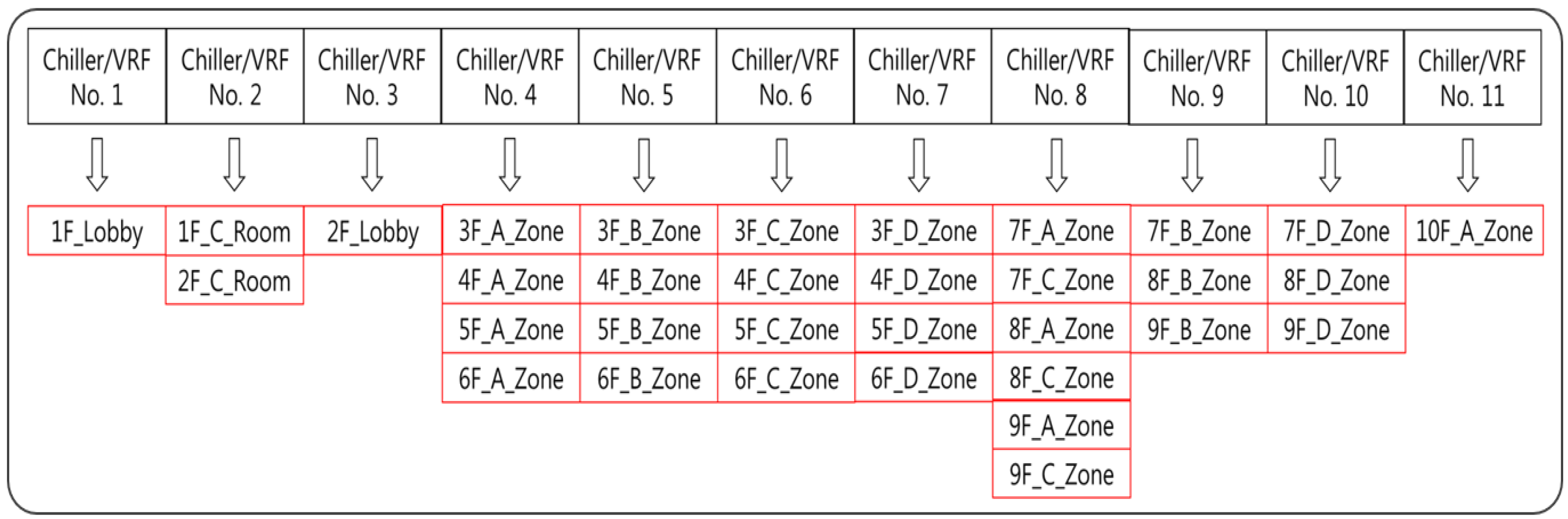
| Capacity (kW) | |||||||||
|---|---|---|---|---|---|---|---|---|---|
| VRF No. 1 | VRF No. 2 | VRF No. 3 | VRF No. 4 | VRF No. 5 | VRF No. 6 | ||||
| 83.1 | 52.8 | 83.3 | 112.3 | 111.7 | 112.8 | ||||
| VRF No. 7 | VRF No. 8 | VRF No. 9 | VRF No. 10 | VRF No. 11 | |||||
| 111.6 | 178.4 | 82.2 | 82.0 | 67.4 | |||||
| Components | Unit | Input Value |
|---|---|---|
| Occupants | Person/Area | 0.078 person/m2 |
| Lighting | Watts/Area | 21.52 W/m2 |
| Electric Equipment | Watts/Area | 16.14 W/m2 |
| Cooling Schedule | Occupants (Ratio) | Lighting (Ratio) | Electric Equipment (Ratio) |
|---|---|---|---|
| Weekdays | 00:00~06:00 (0.000) 06:00~22:00 (0.500) 22:00~23:59 (0.025) | 00:00~23:59 (0.250) | 00:00~23:59 (1.000) |
| Saturday | 00:00~06:00 (0.000) | 00:00~06:00 (0.012) | 00:00~06:00 (0.300) |
| 06:00~08:00 (0.500) | 06:00~08:00 (0.025) | 06:00~08:00 (0.400) | |
| 08:00~12:00 (0.150) | 08:00~12:00 (0.075) | 08:00~12:00 (0.500) | |
| 12:00~17:00 (0.050) | 12:00~17:00 (0.037) | 12:00~17:00 (0.350) | |
| 17:00~23:59 (0.000) | 17:00~23:59 (0.012) | 17:00~23:59 (0.300) | |
| Sunday | 00:00~23:59 (0.000) | 00:00~23:59 (0.012) | 00:00~23:59 (0.300) |
| Category | Input Value |
|---|---|
| Simulation program | EnergyPlus v8.5 |
| Site/weather location | Seoul/Republic of Korea |
| Window-to-wall ratio | 40% |
| Chiller based conventional AHU/water-cooled VRF schedule | 24 h |
| Cooling setpoint | 26 °C |
| COP | 4.787 |
| Pump motor efficiency | 90% |
| Infiltration | 0.0003167 m3/s-m2 |
© 2018 by the authors. Licensee MDPI, Basel, Switzerland. This article is an open access article distributed under the terms and conditions of the Creative Commons Attribution (CC BY) license (http://creativecommons.org/licenses/by/4.0/).
Share and Cite
Kang, I.; Lee, K.H.; Lee, J.H.; Moon, J.W. Artificial Neural Network–Based Control of a Variable Refrigerant Flow System in the Cooling Season. Energies 2018, 11, 1643. https://doi.org/10.3390/en11071643
Kang I, Lee KH, Lee JH, Moon JW. Artificial Neural Network–Based Control of a Variable Refrigerant Flow System in the Cooling Season. Energies. 2018; 11(7):1643. https://doi.org/10.3390/en11071643
Chicago/Turabian StyleKang, Insung, Kwang Ho Lee, Je Hyeon Lee, and Jin Woo Moon. 2018. "Artificial Neural Network–Based Control of a Variable Refrigerant Flow System in the Cooling Season" Energies 11, no. 7: 1643. https://doi.org/10.3390/en11071643
APA StyleKang, I., Lee, K. H., Lee, J. H., & Moon, J. W. (2018). Artificial Neural Network–Based Control of a Variable Refrigerant Flow System in the Cooling Season. Energies, 11(7), 1643. https://doi.org/10.3390/en11071643