A New Hybrid Approach Using the Simultaneous Perturbation Stochastic Approximation Method for the Optimal Allocation of Electrical Energy Storage Systems


Abstract
1. Introduction
- A distributed storage is considered to catch the potential advantages brought by EESSs in an unbalanced distribution system.
- The procedure accounts for many economic and technical aspects of the EESSs allocation.
- The implementation of the solving algorithm based on the SPSA method allows to considerably shorten the computational time while providing good-quality solutions.
- The inner simplified approach allows it to quickly carry out the daily scheduling of the EESSs, further shortening the computational time.
- The comparison of the obtained results with the results of a Genetic Algorithm (GA) and of an exhaustive procedure gives evidence of the accuracy and of the computational effort reduction.
2. Problem Formulation
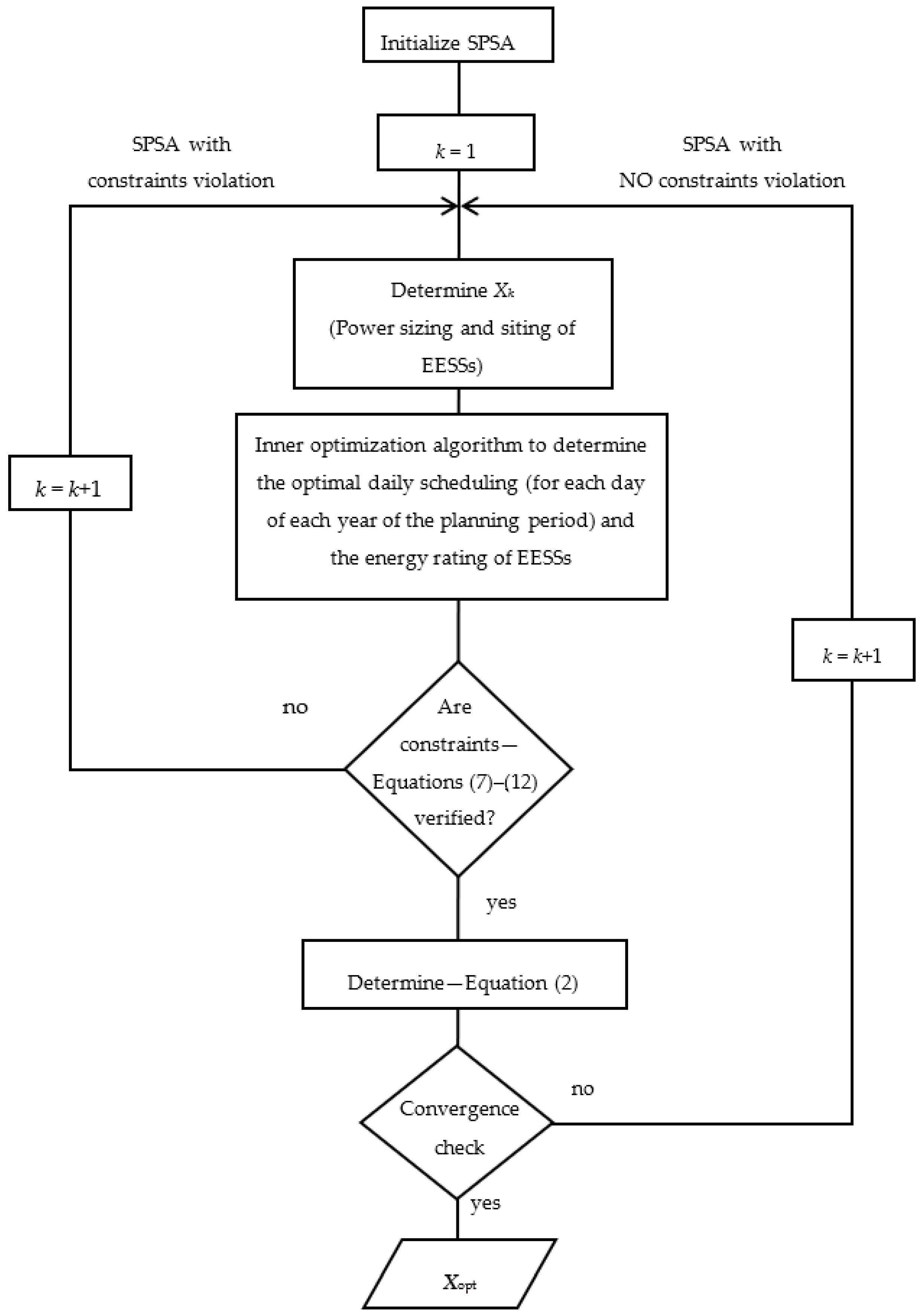
3. Solving Procedure
3.1. The Simultaneous Perturbation Stochastic Approximation Method
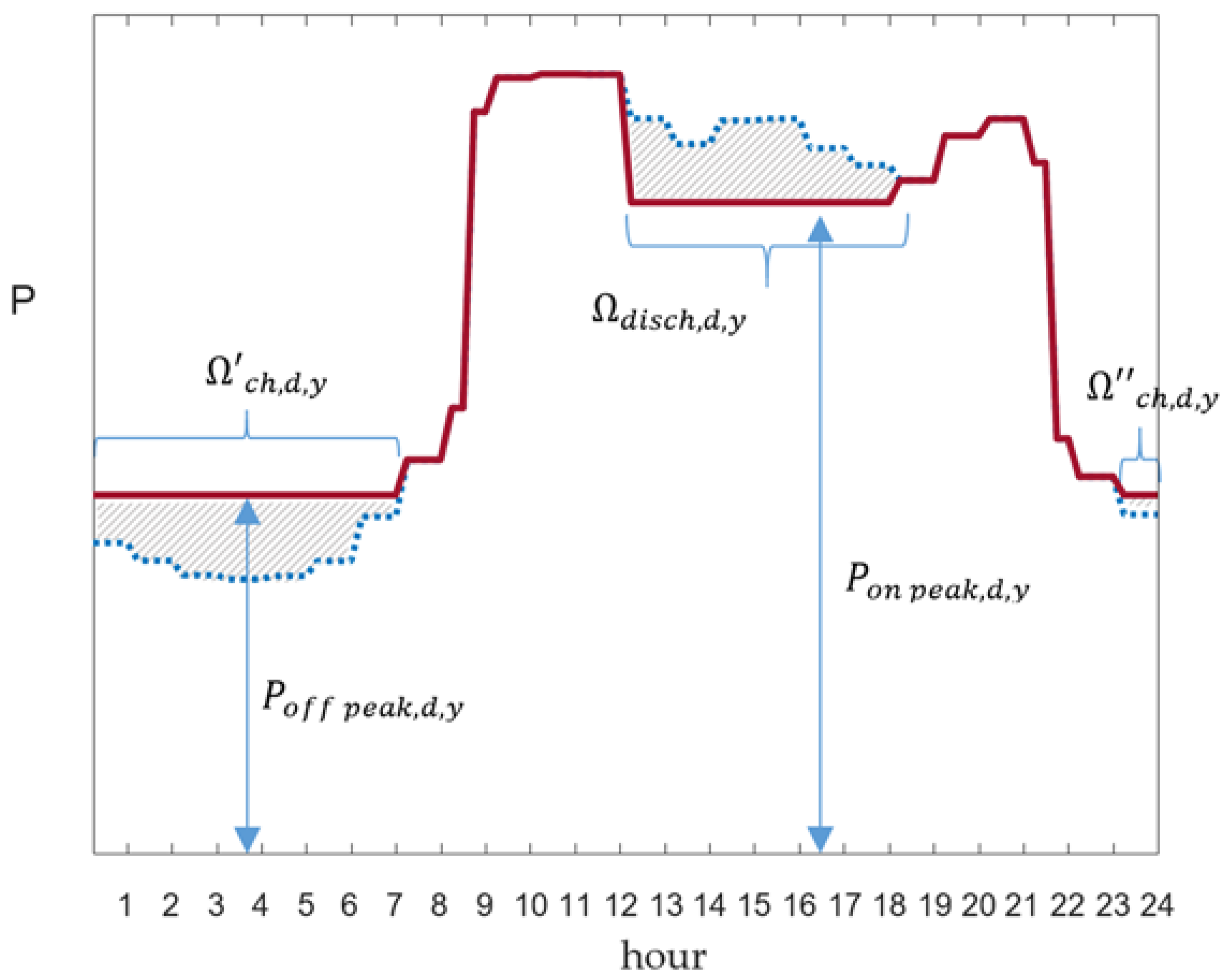
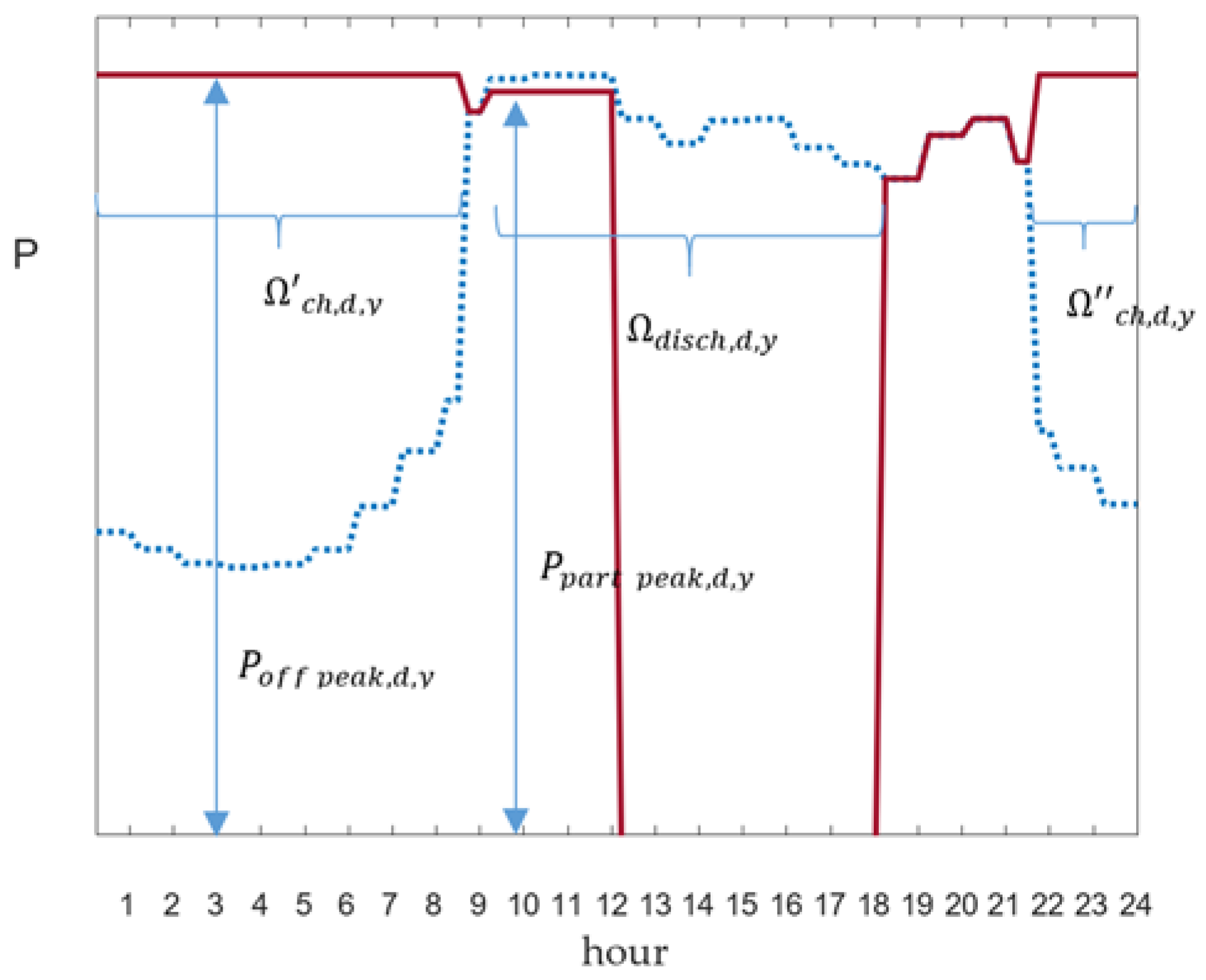
3.2. Inner Algorithm: the EESSs Daily Scheduling
- i
- capacity of the grid: the “updated” daily curves (provided by the sum of the load powers and of the EESS power) do not have to exceed the peak power of the loads,
- ii
- exportation is not allowed: when the EESS is discharging, power cannot flow toward the main grid,
4. Micro Genetic Algorithms
- a control on the fitness improvement provided by the next solution; or
- a maximum number of generated individuals.
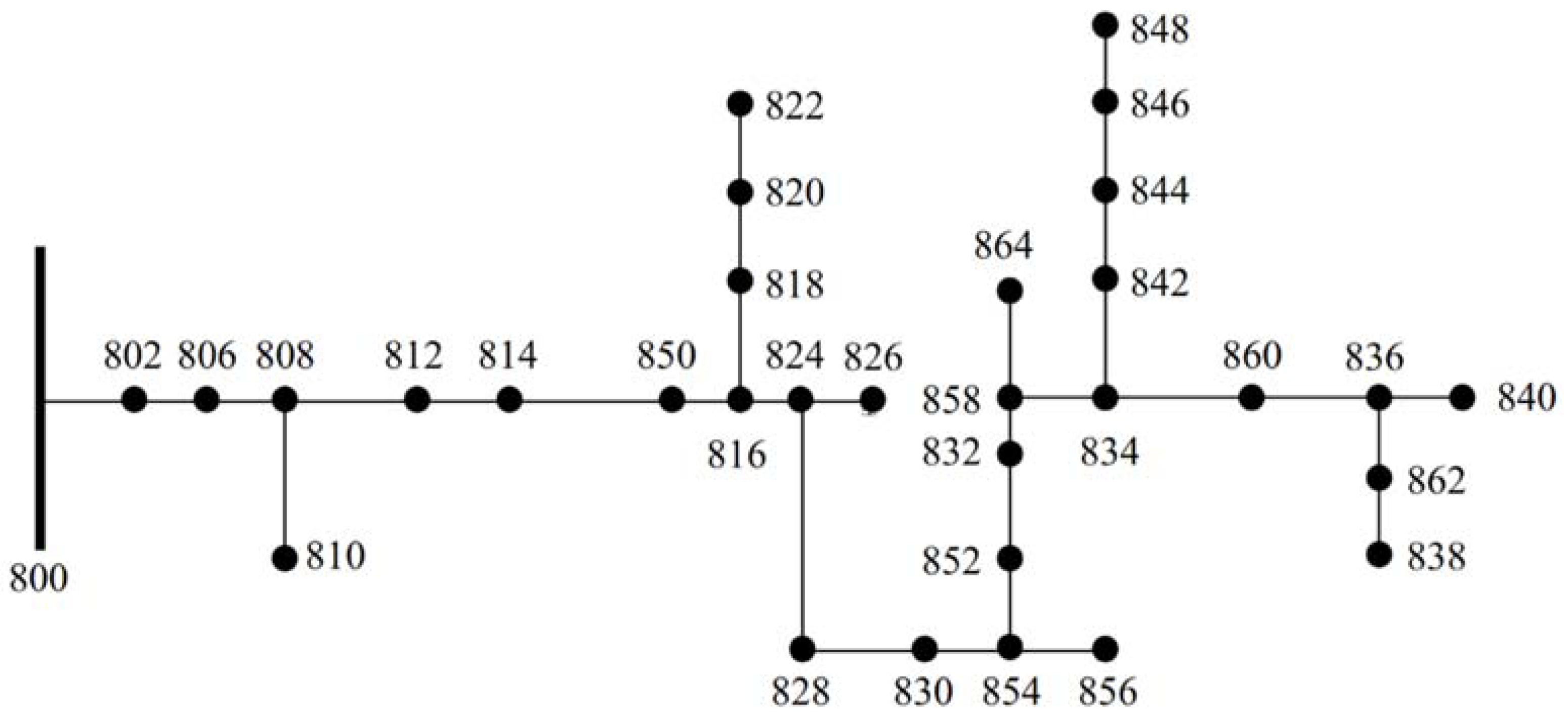
5. Case Study
- Mode 1: The energy storage systems are used only in the summer months: during the off-peak hours they can charge, and during the rest of the day the battery can discharge. The storage systems also exchange the reactive power subject to the constraints of Equation (6).
- Mode 2: For each day of the year, the energy storage systems can charge during the off-peak hours, and they can discharge during the remaining hours. Both active and reactive powers can be exchanged subject to the constraints of Equation (6).
5.1. Analysis of Several Technologies
- Energy and power installation costs
- Electrochemical properties (energy density, power density)
- Costs evolution
- Performances.
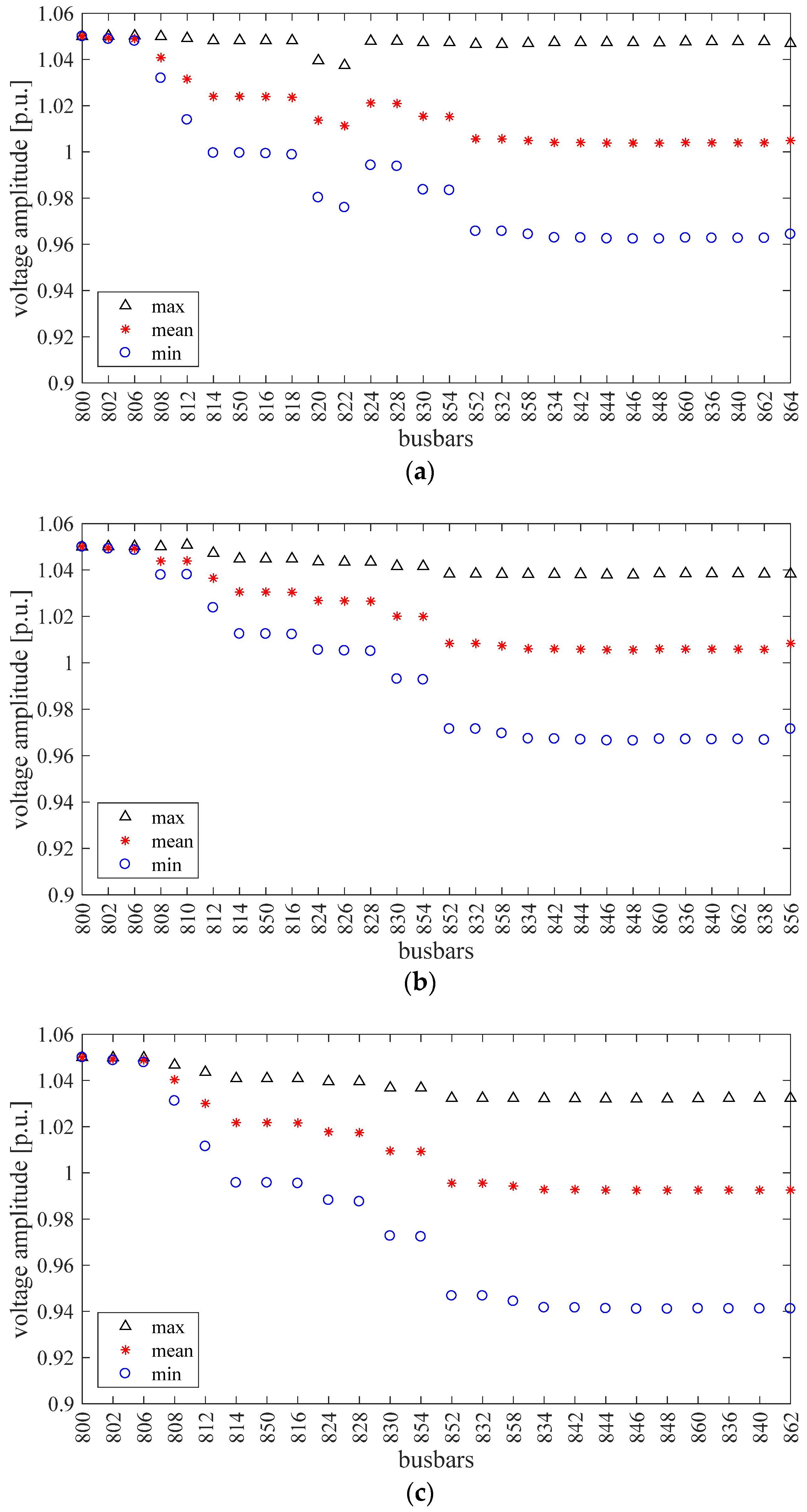
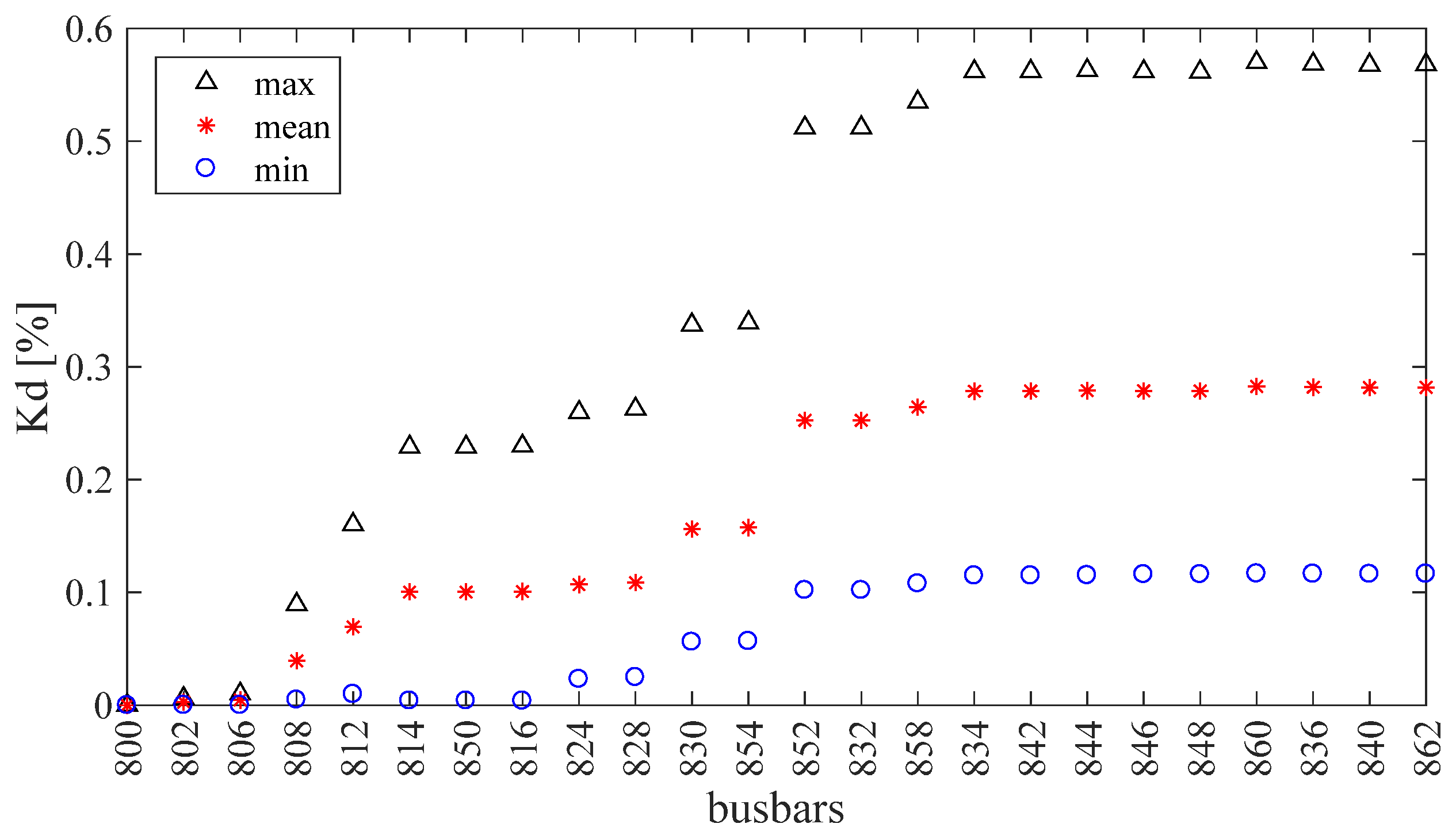
5.2. Results
- the optimal value of the power/energy ratio is always 1/6; this value is adequate for Na-NiCl2 batteries.
- The total size of installed EESSs is 700 kVA (4.2 MWh) for Mode 1 and 650 kVA (3.9 MWh) for Mode 2, respectively.
- The Mode 1 allows it to obtain smaller total costs. These results confirm that there is convenience in using the storage systems only in the most adequate conditions, due to the non-negligible cycling costs.
6. Conclusions
Author Contributions
Funding
Conflicts of Interest
Appendix A. List of Principal symbols
| Discount rate | |
| Rate of change of the electrical energy cost | |
| Efficiency of the electrical energy storage system installed at bus , at hour of the day in the year | |
| Phase of voltage at phase of bus , at hour of the day in the year | |
| kth random perturbation vector | |
| Duration of the time intervals in | |
| Set/index of the busses of the network | |
| Set/index of day | |
| Set/index of hour | |
| Set/index of line | |
| Set/index of bus with electrical energy storage systems | |
| Set/index of year | |
| Constants | |
| Unitary cost of energy | |
| Objective function | |
| kth gradient | |
| Unbalance factor at bus , at hour of the day in the year | |
| Maximum allowable value of unbalance factor | |
| Index of bus phase ( = 1, 2, 3) | |
| Number of replacements of batteries installed at bus | |
| nominal discharging time | |
| maximum value of the nominal discharging time | |
| ith variable | |
| Installation cost of electrical energy storage system for unit of energy | |
| Cost of the energy storage systems installed in the system | |
| Cost of the energy storage system installed at bus | |
| Cost of the energy acquired from the upstream grid in the planning period | |
| Cost of energy provided by the upstream grid, at hour of the day in the year | |
| Size (energy) of the electrical energy storage system installed at bus | |
| Unitary capacity cost of the batteries, at the year | |
| Terms of the three-phase network admittance matrix relating bus with phase and bus with phase | |
| Current flowing in line , at hour of the day in the year | |
| Ampacity of line | |
| Number of buses | |
| Active power at phase of the slack bus, at hour of the day in the year | |
| Active power at phase of bus , at hour of the day in the year | |
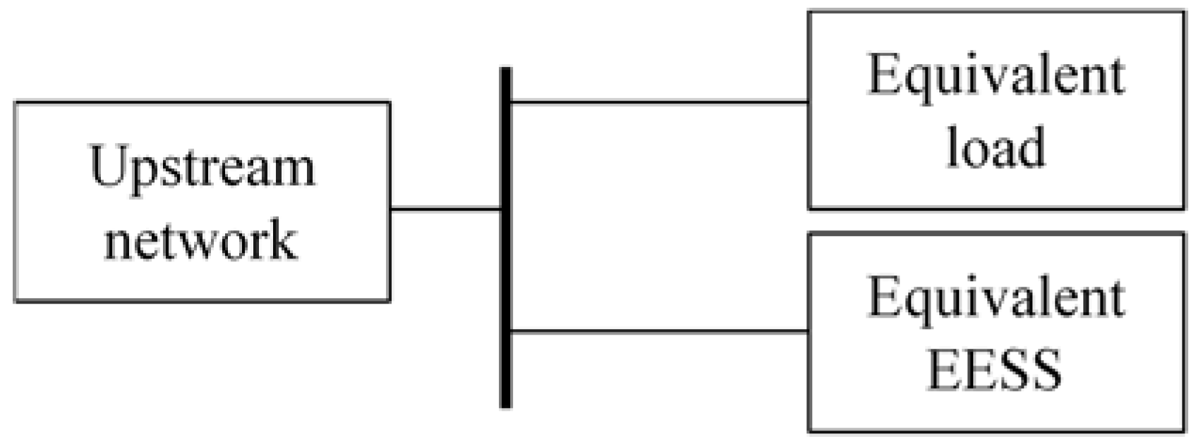
| Power rating of the equivalent EESS (Figure 2) | |
| Constant value of load and equivalent EESS power during the on peak hours | |
| Constant value of load and equivalent EESS power during the off peak hours | |
| Size (power) of the electrical energy storage system installed at bus | |
| Active power of the electrical energy storage system installed at bus , at hour of the day in the year | |
| Active power of the equivalent electrical energy storage system, at hour of the day in the year | |
| Present value | |
| Reactive power at phase of bus , at hour of the day in the year | |
| Reactive power of the electrical energy storage system installed at bus , at hour of the day in the year | |
| Rating of the interfacing transformer | |
| Rating of the AC/DC interfacing converter of the electrical energy storage system installed at bus s | |
| Initial cost of electrical energy storage system for unit of power | |
| Magnitude of voltage phase p of bus b, at hour h of the day d in the year y | |
| Minimum and maximum allowable value of voltage magnitude | |
| Vector of variables |
References
- Luo, X.; Wang, J.; Dooner, M.; Clarke, J. Overview of current development in electrical energy storage technologies and the application potential in power system operation. Appl. Energy 2015, 137, 511–536. [Google Scholar] [CrossRef]
- Chua, K.H.; Lim, Y.S.; Taylor, P.; Morris, S.; Wong, J. Energy Storage System for Mitigating Voltage Unbalance on Low-Voltage Networks with Photovoltaic Systems. IEEE Trans. Power Deliv. 2012, 27, 1783–1790. [Google Scholar] [CrossRef]
- Chen, C.; Duan, S.; Cai, T.; Liu, B.; Hu, G. Optimal Allocation and Economic Analysis of Energy Storage System in Microgrids. IEEE Trans. Power Electron. 2011, 26, 2762–2773. [Google Scholar] [CrossRef]
- Zheng, Y.; Dong, Z.Y.; Luo, F.J.; Meng, K.; Qiu, J.; Wong, K.P. Optimal Allocation of Energy Storage System for Risk Mitigation of DISCOs with High Renewable Penetrations. IEEE Trans. Power Syst. 2014, 29, 212–220. [Google Scholar] [CrossRef]
- Mateo, C.; Reneses, J.; Rodriguez-Calvo, A.; Frías, P.; Sánchez, Á. Cost–benefit analysis of battery storage in medium-voltage distribution networks. IET Gener. Transm. Distrib. 2016, 10, 815–821. [Google Scholar] [CrossRef]
- Xiao, J.; Zhang, Z.; Bai, L.; Liang, H. Determination of the optimal installation site and capacity of battery energy storage system in distribution network integrated with distributed generation. IET Gener. Transm. Distrib. 2016, 10, 601–607. [Google Scholar] [CrossRef]
- Xiong, P.; Singh, C. Optimal Planning of Storage in Power Systems Integrated with Wind Power Generation. IEEE Trans. Sustain. Energy 2016, 7, 232–240. [Google Scholar] [CrossRef]
- Nick, M.; Cherkaoui, R.; Paolone, M. Optimal Allocation of Dispersed Energy Storage Systems in Active Distribution Networks for Energy Balance and Grid Support. IEEE Trans. Power Syst. 2014, 29, 2300–2310. [Google Scholar] [CrossRef]
- Nick, M.; Cherkaoui, R.; Paolone, M. Optimal siting and sizing of distributed energy storage systems via alternating direction method of multipliers. Int. J. Electr. Power Energy Syst. 2015, 72, 33–39. [Google Scholar] [CrossRef]
- Nick, M.; Cherkaoui, R.; Paolone, M. Optimal Planning of Distributed Energy Storage Systems in Active Distribution Networks Embedding Grid Reconfiguration. IEEE Trans. Power Syst. 2017, in press. [Google Scholar] [CrossRef]
- Marra, F.; Tarek-Fawzy, Y.; Bülo, T.; Blaži, B. Energy Storage Options for Voltage Support in Low-Voltage Grids with High Penetration of Photovoltaic. In Proceedings of the IEEE PES Innovative Smart Grid Technologies (ISGT), Berlin, Germany, 14–17 October 2012. [Google Scholar]
- Saboori, H.; Hemmati, R.; Jirdehi, M.A. Reliability improvement in radial electrical distribution network by optimal planning of energy storage systems. Energy 2015, 93, 2299–2312. [Google Scholar] [CrossRef]
- Alnaser, S.W.; Ochoa, L.F. Optimal Sizing and Control of Energy Storage in Wind Power-Rich Distribution Networks. IEEE Trans. Power Syst. 2016, 31, 2004–2013. [Google Scholar] [CrossRef]
- Li, Q.; Ayyanar, R.; Vittal, V. Convex Optimization for DES Planning and Operation in Radial Distribution Systems with High Penetration of Photovoltaic Resources. IEEE Trans. Sustain. Energy 2016, 7, 985–995. [Google Scholar] [CrossRef]
- Babacan, O.; Torre, W.; Kleissl, J. Siting and sizing of distributed energy storage to mitigate voltage impact by solar PV in distribution systems. Sol. Energy 2017, 146, 199–208. [Google Scholar] [CrossRef]
- Motalleb, M.; Reihani, E.; Ghorbani, R. Optimal placement and sizing of the storage supporting transmission and distribution networks. Renew. Energy 2016, 94, 651–659. [Google Scholar] [CrossRef]
- Carpinelli, G.; Mottola, F.; Proto, D.; Russo, A.; Varilone, P. A Hybrid Method for Optimal Siting and Sizing of Battery Energy Storage Systems in Unbalanced Low Voltage Microgrids. Appl. Sci. 2018, 8, 455. [Google Scholar] [CrossRef]
- Zidar, M.; Georgilakis, P.S.; Hatziargyriou, N.D.; Capuder, T.; Škrlec, D. Review of energy storage allocation in power distribution networks: applications, methods and future research. IET Gener. Transm. Distrib. 2016, 10, 645–652. [Google Scholar] [CrossRef]
- Grover-Silva, E.; Girard, R.; Kariniotakis, G. Optimal sizing and placement of distribution grid connected battery systems through an SOCP optimal power flow algorithm. Appl. Energy 2017, in press. [Google Scholar] [CrossRef]
- Mottola, F.; Proto, D.; Russo, A.; Varilone, P. Planning of Energy Storage Systems in Unbalanced Microgrids. In Proceedings of the 7th IEEE International Conference on Innovative Smart Grid Technologies (IEEE PES ISGT Europe), Torino, Italy, 26–29 September 2017. [Google Scholar]
- Spall, J.C. A Stochastic Approximation Technique for Generating Maximum Likelihood Parameter Estimates. In Proceedings of the American Control Conference, Minneapolis, MN, USA, 10–12 June 1987; pp. 1161–1167. [Google Scholar]
- Spall, J.C.; Wiley, J. Introduction to Stochastic Search and Optimization; John Wiley & Sons: New York, NY, USA, 2003; pp. 176–207. [Google Scholar]
- Spall, J. C. An Overview of the Simultaneous Perturbation Method for Efficient Optimization. Johns Hopkins APL Tech. Dig. 1998, 19, 482–492. [Google Scholar]
- Arrillaga, J.; Watson, N.R. Computer Modelling of Electrical Power Systems, 2nd ed.; John Wiley & Sons, Wiley: Chichester, UK, 2001. [Google Scholar]
- Bangerth, W.; Klie, H.; Wheeler, M.F.; Stoffa, P.L.; Sen, M.K. On optimization algorithms for the reservoir oil well placement problem. Comput. Geosci. 2006, 10, 303–319. [Google Scholar] [CrossRef]
- Wang, I.J.; Spall, J.C. Stochastic optimization with inequality constraints using simultaneous perturbations and penalty functions. Proceedings the 42nd IEEE Conference on Decision and Control, Maui, HI, USA, 9–12 Decembar 2003; pp. 3808–3813. [Google Scholar]
- Carpinelli, G.; Noce, C.; Russo, A.; Varilone, P. A Probabilistic Approach for Optimal Capacitor Placement in a Distribution System Using Simultaneous Perturbation Stochastic Approximation. In Proceedings of the CIRED International Conference, Lyon, France, 15–18 June 2015. [Google Scholar]
- Delfanti, M.; Granelli, G.P.; Marannino, P.; Montagna, M. Optimal capacitor placement using deterministic and genetic algorithms. IEEE Trans. Power Syst. 2000, 15, 1041–1046. [Google Scholar] [CrossRef]
- Kersting, W.H. Radial Distribution Test Feeders. In Proceedings of the IEEE Power Engineering Society Winter Meeting, Columbus, OH, USA, 28 January–1 February 2001; pp. 908–912. [Google Scholar]
- Rates-Pacific Gas and Electric Company. Available online: http://www.pge.com/tariffs/ (accessed on 1 June 2018).
- Di Lembo, G.; Noce, C.; Petroni, P. Reduction of power losses and CO2 emissions: accurate network data to obtain good performances of DMS Systems. In Proceedings of the CIRED International Conference, Prague, Czech Republic, 8–11 June 2009. [Google Scholar]
- Data Center Architecture Overview. Available online: https://www.irena.org/-/media/Files/IRENA/Agency/Events/2017/Mar/15/2017_Kairies_Battery_Cost_and_Performance_01.pdf?la=en&hash=773552B364273E0C3DB588912F234E02679CD0C2 (accessed on 7 June 2018).
- NGK Insulators. Available online: https://www.ngk.co.jp/nas (accessed on 7 June 2018).
- Moseley, P.T.; Rand, D.A.J. High-Temperature Sodium Batteries for Energy Storage. In Electrochemical Energy Storage for Renewable Sources and Grid Balancing; Elsevier: Amsterdam, The Netherlands, 2015. [Google Scholar]


| Summer Tariff | ||
| Period | price ($/MWh) | |
| On-peak | 12:00 noon to 6:00 pm | 542.04 |
| Part-Peak | 8:30 am to 12:00 noon and 6:00 pm to 9:30 pm | 252.90 |
| Off-Peak | 9:30 pm to 8:30 am | 142.54 |
| Winter Tariff | ||
| Period | price ($/MWh) | |
| On-Peak | 8:30 am to 9:30 pm | 161.96 |
| Off-Peak | 9:30 pm to 8:30 am | 132.54 |
| Storage systems | Location and Size |
|---|---|
| Three-phase storage systems | 150 kVA/900 kWh at bus #806 150 kVA/900 kWh at bus #836 150 kVA/900 kWh at bus #844 150 kVA/900 kWh at bus #860 |
| Single-phase storage systems | 50 kVA/300 kWh at bus #810 50 kVA/300 kWh at bus #818 |
| Storage systems | Location and Size |
|---|---|
| Three-phase storage systems | 150 kVA/900 kWh at bus #806 150 kVA/900 kWh at bus #844 300 kVA/1800 kWh at bus #858 |
| Single-phase storage systems | 50 kVA/300 kWh at bus #818 |
| Mode | Objective Function (p.u.) |
|---|---|
| Mode 1 | 0.8974 |
| Mode 2 | 0.9447 |
| Configuration | Objective Function (p.u.) | |
|---|---|---|
| Operating Mode 1 | Operating Mode 2 | |
| Optimal configuration obtained for Mode 1 | 0.8974 | 0.9466 |
| Optimal configuration obtained for Mode 2 | 0.8991 | 0.9447 |
| Storage Systems | Location and Size |
|---|---|
| Three-phase storage systems | 150 kVA/900 kWh at bus #802 150 kVA/900 kWh at bus #836 150 kVA/900 kWh at bus #844 150 kVA/900 kWh at bus #852 |
| Single-phase storage systems | 50 kVA/300 kWh at bus #810 50 kVA/300 kWh at bus #820 |
© 2018 by the authors. Licensee MDPI, Basel, Switzerland. This article is an open access article distributed under the terms and conditions of the Creative Commons Attribution (CC BY) license (http://creativecommons.org/licenses/by/4.0/).
Share and Cite
Carpinelli, G.; Mottola, F.; Noce, C.; Russo, A.; Varilone, P. A New Hybrid Approach Using the Simultaneous Perturbation Stochastic Approximation Method for the Optimal Allocation of Electrical Energy Storage Systems. Energies 2018, 11, 1505. https://doi.org/10.3390/en11061505
Carpinelli G, Mottola F, Noce C, Russo A, Varilone P. A New Hybrid Approach Using the Simultaneous Perturbation Stochastic Approximation Method for the Optimal Allocation of Electrical Energy Storage Systems. Energies. 2018; 11(6):1505. https://doi.org/10.3390/en11061505
Chicago/Turabian StyleCarpinelli, Guido, Fabio Mottola, Christian Noce, Angela Russo, and Pietro Varilone. 2018. "A New Hybrid Approach Using the Simultaneous Perturbation Stochastic Approximation Method for the Optimal Allocation of Electrical Energy Storage Systems" Energies 11, no. 6: 1505. https://doi.org/10.3390/en11061505
APA StyleCarpinelli, G., Mottola, F., Noce, C., Russo, A., & Varilone, P. (2018). A New Hybrid Approach Using the Simultaneous Perturbation Stochastic Approximation Method for the Optimal Allocation of Electrical Energy Storage Systems. Energies, 11(6), 1505. https://doi.org/10.3390/en11061505