Abstract
Economic load dispatch (ELD) is an important optimization problem for operating and controlling modern power systems, and if ELD is effectively executed, power systems work stably and economically. The main objective of this paper is to develop a novel method to solve the ELD with the purpose of minimizing the total fuel cost of all available generating units while requirements are to satisfy all constraints regarding thermal units, generators, and transmission power networks. The proposed high performance cuckoo search algorithm (HPCSA) is developed from the efficient technique for the second new solution generation of conventional cuckoo search algorithm (CCSA), called adaptive mutation technique. This proposed technique diversifies the local search ability based on a new comparison criterion. The HPCSA is verified on difference systems under special conditions, namely the 10-unit system with multi fuels, 15-unit system considering prohibited operating zones, and three IEEE systems with 30, 57, and 118 buses considering transmission power network constraints. The specific evaluation of the HPCSA is compared to that of Lagrange optimization-based methods (LMS), neural network-based methods (NNMS), CCSA, and other popular methods such as Particle swarm optimization (PSO) variants, Differential evolution (DE) variants, Genetic Algorithm (GA) variants, and state-of-the-art methods. In comparison with CCSA, the proposed method is always more effective and more robust since the proposed method can find most solutions with better quality and faster convergence speed. In comparison with LMS and NNMS, the proposed method can also find solutions with approximate or equal quality. In comparison with popular methods and state-of-the-art methods, the proposed method has more potential since it can reach faster convergence to valid solutions with approximate or better quality. Consequently, it can be concluded that the proposed HPCSA is an effective optimization tool for dealing with ELD problems.
1. Introduction
Over the past decades, a high number of researchers have been devoted to solving optimization problems in engineering by applying conventional optimization algorithms or proposing improved algorithms. Even though there are some wider application areas where these works are applied, this study narrows down to the economic load dispatch (ELD) problem, which is to minimize the total electricity generation fuel cost of all thermal generating units and to satisfy all constraints of the units and other constraints related to transmission power networks [1,2]. For the considered problems, we consider five systems, in which the first system, namely the 10-unit system, considers multiple types of fuel; the second system, the 15-unit system, considers single fuel, prohibited zones, and spinning reserve for power systems; and the three remaining systems, IEEE 30, 57, and 118 buses, power networks and consider single fuel and all constraints.
So far, a large number of methods have been successfully applied for dealing with the five cases of the problem in which methods applied to the case of multi-fuel options are conventional Hopfield neural network (HNN) [3], hierarchical approach (HA) [4], adaptive Hopfield neural network (AHNN) [5], improved Lagrangian neural network (ILNN) [6], hybrid real-coded genetic algorithm (HRCGA) [7], differential evolution (DE) [8], modified evolutionary programming (MEP) [9], artificial immune system algorithm (AIS) [10] and hybrid differential evolution and dynamic programming (HDEDP) [11], and cuckoo search algorithm (CSA) [12]. Among these methods, ones based on neural network and numerical method have the same disadvantages, such as the hard task of tuning control parameters and stopping application for systems with non-differentiable functions. On the contrary, the remaining methods, DE, HRCGA, AISA, and CSA, can overcome such drawbacks, but they cope with other restrictions much depending on randomization and taking much time for tuning control parameters. Among methods belonging to neural networks, IALHN can be considered the most powerful method while CSA can be the most promising meta-heuristic method in the second group.
For the second system, with consideration of prohibited operating zones (POZ) constraints, several methods as CSA [12], the combination of decomposition method and Lagrange relaxation (DLR) [13], lambda iteration method (LIM) [14], particle swarm optimization (PSO) [15], improved quantum-inspired evolutionary algorithm (IQIEA) [16], and improved augmented Lagrange-Hopfield network (IALHN) [17] have been successfully applied with promising results, but most of these methods have not been evaluated in terms of convergence speed because iterations and execution time have not been reported. It is clear that the systems considering POZ constraints have attracted both conventional algorithms and recent meta-heuristic algorithms. Among the mentioned methods, DLR and LIM are the first two methods applied for handling such complicated constraints, and they have obtained optimal solutions with higher objective function than most other remaining methods excluding the comparison of LIM with PSO.
For IEEE 30, 57, and 118 buses power networks, complicated constraints of transmission power networks such as power and voltage limitations of generators, limitations of transformer tap, limitations of capacitor banks, capacity of transmission lines, and active and reactive power balance are taken into consideration. On the other hand, for the cases of considering the constraints associated with transmission power networks, the ELD problem can be also called optimal power flow (OPF) problem. For the complicated OPF problem, the three most popular IEEE systems with 30, 57 and 118 buses have been employed to test performance of optimization methods in terms of the ability to handle all constraints, quality of solutions, and processing speed. Most methods are the family of meta-heuristic algorithms in which conventional methods, modified methods, combination of two different methods, and hybrid methods have been developed widely. In fact, there have been a huge number of applied methods such as the integration of improved genetic algorithm and effective decoupled quadratic load flow (IGA-EDQLF) [18], hybrid IGA with incremental power flow model (HIGA) [19], HIGA with boundary method (HIGA-BM) [20], differential evolution [21,22], conventional PSO [23], Evolving ant direction particle swarm optimization (EADPSO) [24], PSO with Pseudo-Gradient and constriction factor (PG-CF-PSO) [25], Biogeography-based optimization algorithm (BBOAA) [26] and adaptive real-coded biogeography-based optimization algorithm (ARCBBOA) [27], teaching–learning-based optimization algorithm (TLBO) [28], improved TLBO (ITLBO) [29], gravitational search algorithm (GSA) [30], Artificial bee colony algorithm (ABCA) [31], Grey wolf optimizer (GWO) [32], modified electromagnetism-like mechanism algorithm (MELMA) [33], modified Colliding Bodies Optimization algorithm (MCBOA) [34], moth swarm algorithm (MSA) [35], improved imperialist competitive algorithm (IICA) [36], cuckoo optimization algorithm (COA) [37], Gaussian bare-bones imperialist competitive algorithm (GBBICA) [38], and mathematical programming algorithm (MPA) [39]. In [18,19,20], different variants of GA have been developed in which GA has been improved first and then combined with another method for handling constraints of OPF problem. In fact, Decoupled Quadratic Load Flow has been used in [18] for dealing with OPF problem while IGA has acted as an optimization tool for searching optimal solutions. Hybrid IGA has been applied in both [19,20] while incremental power flow model has been employed in [19], but boundary method has been used in [20]. Conventional PSO and two other improved versions have been suggested, respectively, for each OPF problem in [23,24,25]. In [19], five velocity-updating formulas have been proposed for EADPSO while ant colony search (ACS) has acted as operator for choosing the most appropriate model for each solution. Contrary, EADPSO and PG-CF-PSO have determined more effective direction for updating velocity by using pseudo-gradient theory and used constriction factor (CF) for focusing on potential search zone. The final comparison results have revealed that EADPSO has become more efficient than conventional PSO but less effective than PG-CF-PSO in terms of solution quality and solution searching speed. The authors in [27,29] have made a big effort in improving the performance of improved versions of BBOA and TLBO. However, the obtained results compared to BBOA and TLBO could not show any superiority of ARCBBOA and ITLBO over BBOA and TLBO. Among remaining methods, MSA is a new method applied to the problem and the comparison results show its strong search ability and stand out over other methods including most above-mentioned methods.
In order to solve the above-mentioned complicated problem, this paper proposes a method to modify the conventional cuckoo search algorithm, namely, the high-performance cuckoo search algorithm (HPCSA). In this paper, the proposed HPCSA is first developed by carrying an adaptive mutation technique with two modifications of the original mutation of conventional cuckoo search algorithm (CCSA) [40]. The first proposes two more equations for updating new solutions, adding to the original mutation model. However, only one out of the three equations needs to be determined for using the adaptive mutation technique for each considered solution depending on the solution’s fitness function value. Thus, the second is proposed to establish a decision of using the most appropriate equation for each solution by comparing the fitness function index of each solution compared to the fitness of the best solution and the average fitness index of all solutions compared to the best solution. The second modification is used for the purpose of supporting the first one effectively in its function, so that it can produce high quality solutions. Through the adaptive mutation technique, the proposed method can diversify its search due to exploiting local search and global search in between small and large zones.
The proposed method and CCSA are implemented based on the numerical results through the tests on other systems with different types of objective functions and adifferent set of constraints to demonstrate the effectiveness and robustness of the proposed technique. In addition, the proposed method is also compared to other existing methods, and then, its efficiency is analyzed and concluded. The main contributions to power system optimization field are as follows:
- (i)
- Point out drawbacks of conventional Cuckoo search algorithm clearly and propose improvements on conventional Cuckoo search algorithm effectively
- (ii)
- Present a clear description for handling constraints, namely selection of decision variables and calculation of dependent variables.
- (iii)
- Investigate performance of the proposed method by testing on different systems with different constraints ranging from small-scale systems to large-scale systems, from simple constraint set to complicated constraint set related to thermal generating units and transmission power networks.
This paper is organized as follows: The introduction is presented in Section 1. Section 2 analyzes the economic load dispatch problem formulation. The classical cuckoo search algorithm is recalled, and the proposed method is developed in Section 3. The implementation of proposed method for solving load dispatch problems is introduced in Section 4. The study cases and discussion of the results are given in Section 5 and Appendix A. Finally, the conclusions are stated in Section 6.
2. Analysis for Economic Load Dispatch
2.1. Objective Function
Minimizing the total cost of electricity generation, the objective function of the ELD problem is considered as follows.
where Fi(Pi) the ith fuel cost function, and can be represented in quadratic form as follows [2]:
Considering the valve-point loading effects of the generating units, this fuel cost function has non-convex form, as shown in Equation (3). For better comparison of the complex between the quadratic form without valve point loading effects and the non-convex form with the valve effects, Figure 1 is constructed. As seen from the figure, non-convex form is a challenge for optimization tools.
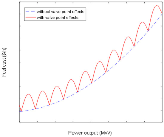
Figure 1.
Fuel cost function for the case of single fuel option.
The fuel cost function for the generating units, which are supplied with multiple fuel options, is mathematically formulated described as follows [21]:
The fuel cost function can combine multiple fuel (MF) options and valve point effects (VPF), as depicted in Figure 2 and expressed by [15]:
where eij and fij are fuel cost coefficients for fuel type jth of unit ith reflecting valve-point effects and mi is the number of fuel types of the thermal unit ith.
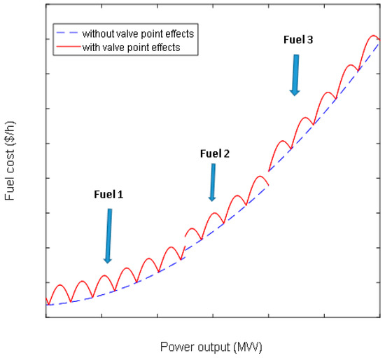
Figure 2.
Fuel cost function for the case of multi-fuel options.
2.2. Constraints
Thermal Generating Unit
Operating Generator constraints: Active and reactive power and working voltage of each generator must satisfy the following inequalities.
where Qi,min and Qi,max are the lower and upper reactive power output of generator ith, respectively; Vi,min and Vi,max are the allowed minimum and maximum voltage of generator ith, respectively; Qi and Vi are the reactive power output and working voltage of generator ith, respectively.
Prohibited Operating Zone constraints: Prohibited operating zones (POZ) exist in the input–output curve of each generator due to the steam valve operation or vibration in its shaft bearing. Therefore, the operating region of a generating unit with POZ will be broken into several isolated feasible sub-regions. The mathematical model of POZ is given in the following formula:
where NPOZi is the number of prohibited zones of unit i; and and are upper and lower bounds for prohibited zone kth of unit ith, respectively; and kth is the POZ number of thermal unit ith.
Spinning reserve constraint: To enhance the stabilization operation of power systems, active power spinning reserve is required and expressed as follows:
where SRP is the total active power that the power systems require for spinning reserve; SRPi is the active power spinning reserve of thermal generating unit ith and calculated as follows:
where SRPi,max is the maximum active power that thermal generating unit ith can contribute to spinning reserve of the power system.
Real power balance constraints: The total real power output of generating units satisfies total load demand plus system power losses
and the total power loss is calculated using Kron’s formula as follows:
In addition, the active power balance constraints can be expressed with respect to terms in transmission lines as follows
where Gij and Bij are the conductance and the susceptance of transmission line ijth connecting bus ith and bus jth.
Reactive power balance constraints: Similar to the constraint model in Equation (14), reactive power balance can be expressed as follows:
in which, the presence of capacitor banks is a result of improving voltage and reduction of power losses; Qdi is reactive power requirement of load at bus ith; and Qci is the reactive power generation of capacitor banks installed at bus ith and is constrained by the following inequality:
where Qci,min and Qci,max are the minimum and maximum reactive power generation of capacitor banks at bus i, respectively, and Nc is the number of buses where capacitors are installed.
Transformer tap constraints: The secondary voltage of a transformer corresponds to transformer tap location. Thus, the tap of the transformer should be set to the predetermined range shown in Equation (17):
where Ti,min and Ti,max are the minimum and maximum transformer tap locations at bus ith respectively; Ti is the current tap location at bus ith; and Nt is the total number of buses where transformers are located.
Load bus voltage constraints: The voltage is one of the most important power quality criteria. Consequently, a stability voltage within the following range must supply the load as follows:
where Vloadi,min and Vloadi,max are the minimum and maximum voltages at bus ith that loads at this bus can work, respectively.
Conductor capacity constraints: The capacity of conductor with respect to the maximum current is also represented as the maximum apparent in power system. The capacity must always satisfy the following rule.
where Ncond represents the total number of conductors (transmission lines); Scondi,max is the capacity of conductor ith; and Scondi is the apparent power flow in conductor ith calculated by:
where Snm and Smn are the apparent power flow from buses nth to mth and from buses mth back to nth, respectively.
3. Approaches
3.1. Classical Cuckoo Search Algorithm
Classical cuckoo search algorithm (CCSA) is composed of two generations for producing new solutions and two times for selection of promising solutions [40]. The first generation is carried out by using Lévy Flights stage and the second generation is done by using mutation operation called discarding identified eggs. The whole search process of CCSA is summarized in the four following steps:
Step 1: Lévy Flights for the first generation is calculated by the following inequality
where α > 0 is the step size ranging from 0 to 1; Lévy (β) is calculated as in Ref. [40]; Xs is solution s that is stored from initialization or from the end of the loop procedure and s = 1, …, Nnest (where Nnest is the number of nests or the number of solutions in the population).
Step 2: Selection for keeping promising solutions: There are two solutions Xs and Ys at each nest s. Thus, only one solution is kept and another must be discarded by using the formula below.
Step 3: Mutation operation for the second generation: The second generation of new solutions is carried out here for improving the solution quality.
where Zr1 and Zr2 are two randomly picked solutions from the current population, randUs is randomly produced within the range from 0 to 1 for solution Us, and PP is a predetermined probability for producing new solutions.
Step 4: Selection for keeping promising solutions: At the end of each iteration, selection operation is repeated for retaining promising solutions.
The best solution among the solution set X = [X1, …, Xs, …, XNnest] is determined by choosing the solution with the lowest fitness function.
3.2. The Proposed Approach
In this section, the proposed HPCSA is developed by pointing out disadvantages of CCSA, and then solutions for overcoming the disadvantage are proposed. In the mutation technique shown in Equation (23), CCSA updates new solutions for current solution Us by using a jumping step, which is the difference between two randomly selected solutions Zr1 and Zr2. Clearly, the use of the three considered solutions can lead to several limitations such as low performance of local search and easily trapping into local optimum. Besides, the mutation of CCSA is always carried out by using the difference of only two random solutions over the search process with Imax iterations. Consequently, the mutation with Equation (23) reduces the diversity of the local search and global search of CCSA. To overcome the drawback, we suggest using the three following mutation modes for the current population.
Among such mutation modes, rand/1 can narrow the search space while rand/2 and rand/3 can reach to larger search zone. The three modes can diversify the search strategy; however, the target is only reached as use of them is appropriate for considered solutions. Here, we classify the three different equations into two groups, small zone search group with rand/1 and large zone search group with rand/2 and rand/3. The condition of using either rand/1 or rand/2 and rand/3 is dependent on the comparison of ∆s and ∆mean, which are shown in Equations (28) and (29).
where Zbest is the best solution among the solution set Z, in which Z = [Z1, Z2, …, ZNnest); FF(Zbest) is the fitness function value of the so-far best solution Zbest. ∆Zs is the fitness index of solution Zs compared to the so-far best solution Zbest; ∆mean is the average fitness index of all solutions compared to the best solution.
For the case of ∆Zs > ∆mean, it means that solution Zs is still far away the current so-far best solution, thus it needs to be search around the current solution Zs with a small zone nearby such solution Zs. On the contrary, for the case that ∆Zs is equal or less than ∆mean, larger jumping step will be applied because current solution is too close to the current best solution. For the latter case, rand/2 or rand/3 is used depending on a random condition of comparing between random number and 0.5. The adaptive mutation is described in detail in Algorithm 1.
| Algorithm 1: The proposed mutation technique |
| If ∆Zs > ∆mean % using rand/1 % rand/1 else if rands > 0.5 % the second condition % rand/2 else % rand/3 end end |
4. Implementation
The proposed HPCSA method is implemented for solving ELD problem as follows.
4.1. Selection of Control Variables for Each Solution
As mentioned in Section 3.1, solution Xs is the initial solution produced at the beginning of the implementation of the proposed HPCSA method. Consequently, control variables should be determined and added in each solution Xs while solution Ys, Zs, and Us have the same control variables as Xs. In the paper, the ELD problem is constructed by using two different sets of constraints of which the first set of constraints neglecting all transmission power networks is comprised, and the second set of constraints that consider the transmission power network. The first set of constraints is composed of Equations (6) and (12), while the second set of constraints consists of all constraints. For the case considering the first constraint set, the control variables are all active power output of (N − 1) thermal generating units while the control variables are Pi (where i = 2, …., N), Vi (where i = 1, …., N), Ti (where i = 1, …., Nt), Qci (where i = 1, …., Nc).
4.2. Processing of Constraints
The equality constraints: For the ELD problem neglecting all constraints in transmission lines, the equality constraint in Equation (6) is exactly met by using the following equation
where PL is calculated by using Equation (7) and the violation of P1 is penalized in fitness function. The detail of calculating P1 can be referred in Ref. [12]. For the case of considering all constraints in transmission lines, all control variables are added in the OPF program, Mathpower for running. Then, all dependent variables, such as P1 (active power output of generator at slack bus), Qi (where i = 1, …, N), Vloadi (where i = 1, …, Nload), and Sbranchi (where i = 1, …, Nbranch) are obtained. Such obtained dependent variables are verified and penalized in fitness function in the case that they are violated.
The inequality constraints: All control variables are checked and repaired. If Xs is higher than the maximum values of control variables, Xs will be assigned to maximum values, and on the contrary, Xs will be set to if it is lower than the minimum values. For the two cases of considering constraints, and are defined as follows
4.3. Construction of Fitness Function
The Fitness function can reflect the objective function quality and the violation level of dependent variables. For the cases of neglecting and considering transmission line constraints, the fitness function is as follows
where KPF is the penalty factor, and the limits related to dependent variables are determined by:
4.4. The Proposed Algorithm
The completely iterative algorithm for implementation of the HPCSA for solving the ELD problem is described in detail below.
- Step 1:
- Select parameters for the HPCSA including three CCSA parameters such as number of nests Nnest, probability of a host bird to discover an alien egg in its nest PP, and maximum number of iterations Imax.
- Step 2:
- Select control variables for each solution by using Section 4.1.
- Produce an initial population randomly so that is always satisfied.
- Step 3:
- Handle equality constraints by using Section “The equality constraints”.
- Calculate fitness function by using either Equation (35) or (36).
- Choose the best solution with the lowest fitness function value.
- Set current iteration to 1, Icur = 1.
- Step 4:
- Produce the first new solution by using Equation (21).
- Dealing with inequality constraints by using Section “The inequality constraints”.
- Step 5:
- Calculate fitness function by using either Equation (35) or (36).
- Perform section operation by using Equation (22).
- Step 6:
- Produce the second new solutions by using proposed Algorithm 1.
- Dealing with inequality constraints by using Section “The inequality constraints”.
- Step 7:
- Calculate fitness function by using either Equation (35) or (36).
- Perform section operation by using Equation (24).
- Step 8:
- Determine the best solution with the lowest fitness function value.
- Step 9:
- Determine the condition to stop the search process: If Icur < Imax, Icur = Icur + 1 and back to Step 4. Otherwise, stop the search process and accept an optimal solution.
5. Case Study and Discussion of the Results
In order to verify the effectiveness, robustness, and convergence speed of the impact of the proposed method, five main power systems, the 10-unit power system, 15-unit power system, IEEE-30 bus power system, IEEE-57 bus power system and IEEE-118 bus power system, are employed. The detail of the five main systems in addition to the selections of population Nnest and the maximum number of iterations Imax are summarized in Table 1. The proposed algorithm is to run 50 independent trials for case 1 and case 2, 100 independent trials for case 3 and case 4, and 200 independent trials for case 5 on a 2.4 GHz PC with 4 GB of RAM.

Table 1.
Description of five main employed power systems and the selections of control parameters.
In addition to the two control parameters, PP is also tuned from 0.1 to 1 with a change of 0.1 for determining the best optimal solution. In order to demonstrate the effectiveness and robustness of the proposed adaptive mutation technique, we also run CCSA for all considered study cases above. For implementation of CCSA, control parameter setting is also carried out similarly as the proposed method.
5.1. Case 1: The 10-Unit System with Multi Fuels and Four Load Cases
In this section, we investigate the performance of the proposed method on a system with 10 units using multi fuel options for four sub-cases in which sub-case 1.1 considers load of 2400 MW, sub-case 1.2 considers load of 2500 MW, sub-case 1.3 considers load of 2600 MW, and sub-case 1.4 considers load of 2700 MW. The data of the system is taken from Ref. [3].
In addition to the implementation of CCSA, we also implement other popular methods such as Particle swarm optimization (PSO), Firefly algorithm (FA), and Flower pollination algorithm (FPA) for solving four subcases of case 1 for comparison. For running the additional methods, we set the population of all methods to 10 whilst the maximum number of iterations is set to 200. The setting aims to balance the number of new solution evaluations between CCSA, the proposed HPCSA, and other methods. Besides, other control parameters of these methods are also set to different values in determined ranges. For instance, two acceleration factors c1 and c2 of PSO are set to different values within 0 and 2.05 with a step size of 0.2, and the probability of FPA has been set to ten values from 0.1 to 1 with a step size of 0.1, while updated step size factor α of FA has been set to 4 values consisting of 0.25, 0.5, 0.75 and 1. The results obtained by these methods and the proposed method are reported in Table 2. In comparison with CCSA, FA, PSO and FPA, it can be seen that the proposed method obtains the lowest minimum cost, and it also obtains the lowest average cost, the lowest highest cost, and the lowest standard deviation, excluding comparison with FPA for subcase 1.3. The indications can confirm the superiority of the proposed method over other ones in terms of the global optimal solution search ability, the stable search ability, and fast convergence to the global solutions.
Table 2.
The results obtained by Firefly algorithm (FA), particle swarm optimization (PSO), flower pollination algorithm (FPA), CCSA and the proposed high performance cuckoo search algorithm (HPCSA) for subcases of case 1.
For more evidence to demonstrate the fast convergence to global optimum of the proposed method over CCSA, one of the best convergence characteristics of CCSA and the proposed method are depicted in Figure 3 for sub-case 1.1 and Figure 4 for sub-case 1.2. The observations from the curves show that the proposed method is always faster than CCSA once the drop of fitness function from the proposed method is significant at the first iterations, and the drop is nearly not clear at the last iterations while CCSA gets not much improvement at the first iterations, and the improvement is still seen at the last iteration. On the other hand, the best fitness function of each run among 50 runs for sub-cases 1.1 and 1.2 are also taken into account in Figure 5 and Figure 6. The figures indicate that most optimal solutions found by the proposed method have approximately equal quality, and the deviation between the worst solution and the best solution is very small, while the fluctuation of CCSA’s solutions is very high. Clearly, the stabilization of optimal solution search ability of the proposed method is superior to that of CCSA. Here, we can see three advantages of the proposed method over CCSA, such as better quality solutions, faster convergence, and more stable search ability. Consequently, it obviously results in a conclusion that the proposed method is much better than CCSA for the system with thermal units using multi-fuel options.
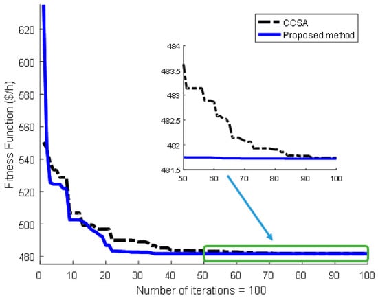
Figure 3.
Fitness function curves iteration obtained by the CCSA and proposed method for sub-case 1.1.
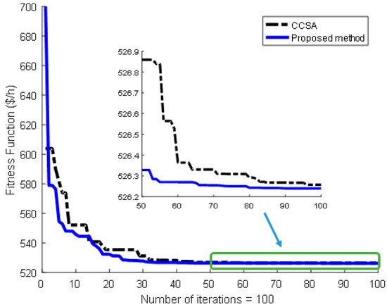
Figure 4.
Fitness function curves iteration obtained by the conventional cuckoo search algorithm (CCSA) and proposed method for sub-case 1.2.
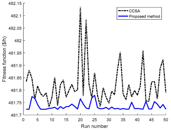
Figure 5.
Fitness function of 50 runs obtained by the CCSA and proposed method in case 1.1.
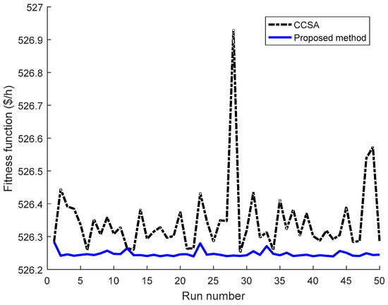
Figure 6.
Fitness function of 50 runs obtained by the CCSA and proposed method in case 1.2.
For further investigation of the effectiveness of the proposed method, comparisons with other methods are tabulated in Table 3. In addition to the best costs, the number of fitness evaluations (NFES), which is equal to (Nnest × Imax) for one generation-based methods and (2 × Nnest × Imax) for two generations-based methods, is also reported in the table. As known, the high population size and/or the high number of iterations can lead to a significant improvement of results. Consequently, a method with lower cost and lower NFES or the same NFES is a more effective method than other compared ones. Based on the comparison criterion, the performance of the proposed method is evaluated for the test case. As observed from the cost for sub-cases, the best cost from the proposed method is less than or approximately equal to that from other ones excluding the cost from AHNN [5] for sub-cases 1.1 and 1.2. Note that power generated by the method [5] is slightly less than the load demand. For comparison, the proposed method has used smaller NFES than all methods whose NFES have been reported. The proposed method has used NFES of 2000 while other methods have used from 3000 to 12,000 in which AISA [10] with 3000, HDEDP [11] with 4000, RCGA [7] and HRCGA [7] with 8000, and DE [8] with 12,000. Clearly, the convergence speed to global optimum of the proposed method is much faster than other ones. There is no evaluation executed on the comparison of the proposed method with others such as HNN [3], HA [4], AHNN [5], ILNN [6], and MEP [9] because HNN [3], HA [4], AHNN [5] and ILNN [6] are not the family of meta-heuristic algorithms, and no information was reported for MEP in [9]. The analysis of the results indicates that the proposed method can yield approximate or better solutions than others while NFES of the proposed method is much lower than that from others. As a result, it can be concluded that the proposed method is more effective than other methods for the system.
Table 3.
The result comparison about cost ($/h) between methods in case 1.
5.2. Case 2: The 15-Unit System Considering Prohibited Operating Zones Constraint
The test system consists of 15 units with four ones such as units 2, 5, 6 and 12 constrained by POZ condition. The system load demand is 2650 MW and the spinning reserve of the system is 200 MW. The data of the system is from [9]. The obtained results by CCSA and proposed methods are summarized in Table 4 while the best fitness convergence and the 50 runs are depicted in Figure 7 and Figure 8. The numerical table can evaluate the best optimal solutions exactly while the figures can support the exact evaluation of the stabilization of the 50 runs. The best cost from the proposed method is $32,544.9704, but the cost from CCSA is $32,544.9834. The average cost from the proposed method is also less than that from CCSA. Figure 7 confirms the faster search of the proposed method compared to CCSA while Figure 8 shows a high fluctuation of CCSA, and most runs of CCSA show much higher cost than those from the proposed method. Thus, the proposed method is more effective than CCSA for the system with POZ constraints.
Table 4.
The obtained results for the CCSA and proposed method in case 2.
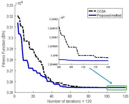
Figure 7.
Fitness function curves iteration obtained by the CCSA and proposed method for case 2.
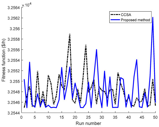
Figure 8.
Fitness function of 50 runs obtained by the CCSA and proposed method in case 2.
In Table 5, the best cost, average cost, maximum cost and NFES from the proposed method are compared to those from other methods such as DM [13], LIM [14], QIEA [16], IQIEA [16] and IALHN [17]. The comparisons of best cost show that the proposed method can converge to a more effective optimal solution with less best cost than DM [13] and LIM [14] while the proposed method also provides less mean cost and less maximum cost than QIEA and IQIEA. Moreover, the value of NFES from the proposed method, 2000, is also smaller than from QIEA and IQIEA, which is 5000. There was no NFES reported for other ones.
Table 5.
The result comparison about cost ($/h) between methods in case 1.
5.3. Case 3: IEEE-30 Bus Power System
The test system is composed of 30 buses consisting of generation 6 buses and 24 load buses, 41 branches, 4 transformers and 9 switchable capacitor banks. The control variables for the system are Pi (i = 1, …, 5), Vi (i = 1, …, 6), Qci (i = 1, …, 9) and Ti (i = 1, …, 4). For the system, there are three sub-cases with three types of fuel cost function where sub-case 3.1 considers single fuel with quadratic form, sub-case 3.2 considers single fuel with nonconvex form and POZ constraints, and sub-case 3.3 considers multi-fuels with piecewise form. The data of the fuel cost functions for these sub-cases are taken from [20,22,41], respectively. The main data belonging to transmission lines of the systems is taken from [25,42].
Figure 9 illustrates the fitness function values of 100 successful runs obtained by CCSA and the proposed method for sub-case 3.1. As seen from the figure, most fitness function values of the proposed method are lower than those of CCSA, and the fluctuation of CCSA is high while the deviation zone of the proposed method is much narrower. In addition, the best costs, mean cost, standard deviation and NFES from CCSA, and the proposed method for the three sub-cases are also given in Table 6 for subcase 3.1, in Table 7 for subcase 3.2 and in Table 8 for subcase 3.3 for comparisons with those from other methods. Observations from such sub-cases show that the proposed method yields better minimum cost than CCSA and most methods excluding MCBOA [34] for sub-cases 3.1, 3.2, and 3.3, HIGA-BM [20], and EADPSO [24] for sub-case 3.3; however, MCBOA has used much high value NFES with 25,000 (for sub-cases 3.1 and 3.2) and 45,000 (for sub-case 3.3) while that of HIGA-BM [20] and EADPSO [24] are 12,000 and 12,500, respectively, but the value from the proposed method is only 2000. Besides, as we check the optimal solution reported in [24], the solution is valid but the exact cost is $956.2325, which is much higher than the reported number of $629.4692. For sub-case 3.2, there is an important note that HIGA-BM [20] has only reported active power of generators for optimal solution, leading to a restriction for checking validation, and the effectiveness of the proposed method cannot be evaluated. The comparison of NFES to the proposed method and other methods indicates that the proposed method is much faster than them because the proposed method used only NFES of 2000 while others have used from NFES of 4560 (HIGA [19]) to 45,000 (MCBOA [34]). For comparisons of mean cost and standard deviation, the three subcases have the same result that those values of other methods are better than those of the proposed method, but the deviation is not insignificant. The results are because of the use of a much higher number of fitness evaluations of other methods.
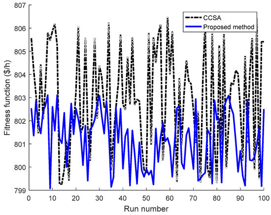
Figure 9.
Fitness function of 100 runs obtained by the CCSA and proposed method in sub-case 3.1.
Table 6.
The result comparison for subcase 3.1.
Table 7.
The result comparison for subcase 3.2.
Table 8.
The result comparison for subcase 3.3.
As a result, it can be concluded that the proposed method is very efficient for solving the system with different cases of fuel cost function. The key variables corresponding to the best fitness function yielded by the proposed method for case 3 are given in Appendix A.
5.4. Case 4: IEEE-57 Bus Power System
In this section, IEEE 57-bus system is employed as a test study to verify the effectiveness and robustness of the proposed method. The system has 80 branches, 57 buses with 7 generator buses and 50 load buses, 15 transformers, and 3 switchable capacitor banks. The main data of the systems is taken from [25,42]. For solving such system, the control variables for the system are Pi (i = 2, …, 7), Vi (i = 1, …, 7), Qci (i = 1, 3), and Ti (i = 1, …, 15). Similar to other reported tables, the best cost, mean cost, and standard deviation together with the value of NFES from the proposed method, CCSA, and other compared methods are summarized in Table 9 for evaluation. In the table, the best costs yielded by the proposed method and CCSA are $41,669.8269 and $41,694.5162, respectively, and the comparison between the two numbers indicates that the optimal solution from the proposed method can provide a lesser cost of $24.69. Again, the fitness function of 100 independent runs obtained by CCSA and the proposed method depicted in Figure 10 illustrates the search ability superiority of the proposed method over CCSA for 100 considered runs. It is clear that the proposed method can find a higher number of good optimal solutions and a fewer number of bad optimal solutions than CCSA because the number of blue points of the proposed method, which is below the number of black points of CCSA, are higher while the number of black points of CCSA, which is more than the blue points, are higher. Thus, the proposed method is more powerful and stronger than CCSA for searching optimal solutions.
Table 9.
The result comparison for case 4.

Figure 10.
Fitness function of 100 runs obtained by the CCSA and proposed method in case 4.
For comparisons with other methods, there is a standout lower cost from ITLBO [29] of $41,638.3822. However, the validation of the reported solution of ITLBO cannot be carried out because ITLBO has reported only active power outputs of generators for decision variables while other remaining decision variables such as capacitor banks’ reactive power output, transformers’ tap setting and generators’ voltage have been omitted. For other comparisons with the second best method, ARCBBOA [27] and the worst method, PSO [25], the optimal solution yielded by the proposed method can provide a cost decreased by $16.17 and $439.89, respectively. Moreover, the comparison of NFES can reflect fast search ability of the proposed method compared to most methods excluding methods in [25] since the proposed method has used NFES of 6000 while that used by other methods is from 14,000 to 110,000. These methods have used 8000 to 105,000 fitness evaluations higher than the proposed method, but the proposed method has used only 1000 fitness evaluations higher than methods in [25]. Most methods have tended to use high value of NFES for improving their performance. For instance, ARCBBOA could provide the second lowest cost, but it has employed a very high NFES of 50,000, and ABCA [31] has owned the four best costs, but its NFES is still high, up to 14,000. For comparison with mean cost and standard deviation, the proposed method reaches smaller values than most methods, excluding EADPSO [24] and ARCBBOA [27]. However, the two methods have used a higher number of fitness evaluations, namely 7500 for EADPSO [24] and 50,000 for ARCBBOA [27] while that of the proposed method is only 6000. Overall, it can lead to a conclusion that the proposed method is efficient for the system. The key variables corresponding to the best fitness function yielded by the proposed method for case 4 are given in Appendix A.
5.5. Case 5: IEEE-118 Bus Power System
In this section, the proposed method is run on the IEEE-118 bus power system with 54 generator buses, 64 load buses, 186 branches, 9 transformers, and 14 capacitor banks. For the largest system, the number of control variables is also the largest with respect to 130 variables such as active power output of 53 generator excluding generator at slack bus 69, voltage of 54 generators, tap value of 9 transformers, and reactive generation of 14 capacitor banks. The whole data of the system is taken from [25,42].
The best cost, mean cost, standard deviation and the value of NFES from the proposed method, CCSA, and other existing methods are tabulated in Table 10 while the fitness function of 200 runs achieved by CCSA and the proposed method are plotted in Figure 11. Comparison with CCSA indicates that the proposed method can provide an optimal solution with less cost than that of CCSA by $254.10, which is equivalent to a reduction of 0.2%. Figure 11 sees that both CCSA and the proposed method have a high fluctuation among the runs; however, the fluctuation level of CCSA is much higher. Besides, the number of blue points below black points is high but the number of blue points above black points is small while most higher points belong to black points of CCSA. Clearly, the proposed method is more powerful than CCSA in searching for an optimal solution for the system. For comparison with other methods, the proposed method still shows its potential search ability, as its optimal solution leads to less cost than most methods excluding MPA [39]; however, there was no optimal solution reported for the result, leading to a failure of verifying the validation. For cost improvement, the proposed method can improve 3.63%, 10.51%, 6.72%, 2.17%, and 0.195% compared to MCBOA [33], PSO [25], PG-CF-PSO [25], COA [37], and CCSA, respectively. Furthermore, mean cost and standard deviation of the proposed method are also less than those from all methods. Comparison of NFES indicates that the proposed method has used the same fitness evaluations of 10,000 as most methods except MCBOA [33] use 22,500 fitness evaluations. In summary, the proposed method can obtain the best optimal solution and the best stabilization of search ability among all compared methods while its fitness evaluations are equal to or less than that of other ones. Consequently, it can be concluded that the proposed method is the most effective method for case 5. The key variables corresponding to the best fitness function yielded by the proposed method for case 5 are given in Appendix A.
Table 10.
The result comparison for case 5.
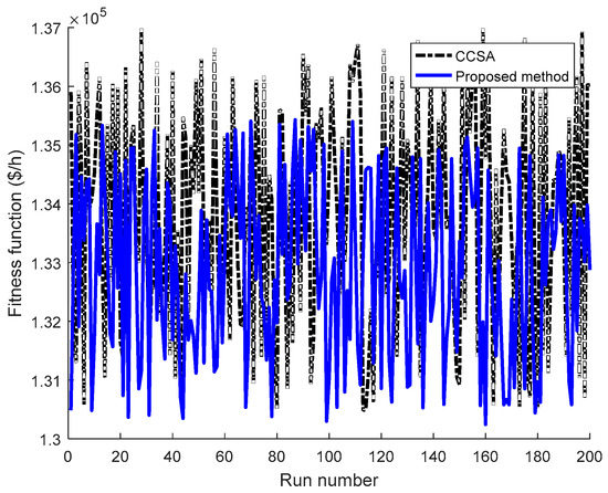
Figure 11.
Fitness function of 100 runs obtained by the CCSA and proposed method in case 5.
5.6. Discussion of Results
In this paper, we propose a high performance cuckoo search algorithm to take advantage of conventional cuckoo search algorithms such as small number of control parameters and easily tuning such control parameters and high possibility of convergence to global optimal solutions. Besides, HPCSA also overcomes disadvantages that CCSA has been facing such as high number of fitness evaluations, low stabilization of searching global optimal solutions, and high standard deviation. In each iteration, CCSA consists of two new solution generations via global search and via local search. The proposed method aims at local search and improves the quality of new solutions obtained by such local search. Thus, the implementation process of such local search of the proposed method is more complicated than that of CCSA, but there is no more additional control parameter needing adjustment.
In comparison with other methods consisting of CCSA and other popular methods, the performance of the proposed HPCSA method has been reflected via the main comparison of the best cost and the number of fitness evaluations. Besides, mean cost and standard deviation have also been added for some cases. On the other hand, t-test reflected by p-value can give evidence of the improvement level of the proposed method over other ones. However, p values of Welch’s t-test for comparison between the proposed and another are obtained only when enough information consisting of mean cost, standard deviation cost, and the number of runs are reported. Furthermore, the p-values can reflect the accurate improvement level of the proposed method over another if the number of runs and the fitness evaluations of the proposed method and compared methods are the same. The mean values and the standard deviation of two methods cannot be compared unless the number of runs of the two methods is equal and the number of fitness evaluations of the two methods is the same. A high number of runs can lead to a more accurate value of mean cost while a high number of fitness evaluations can result in better minimum cost, better mean cost, and better standard deviation cost [43]. In the paper, we have compared the results of the proposed method with more than twenty methods while the number of runs and the fitness evaluation of these compared methods are completely different. Thus, we could not run the proposed method with the same information as each compared method. As a result, we calculate p-values for cases with sufficient conditions. For other cases, we focus on the best cost and the number of fitness evaluations as priority comparison criterion and then mean cost and standard deviation are compared for more accurate evaluation. In Table 11, p-values of Welch’s t-test for comparison of the proposed method and other methods for four subcases of case 1 are given. For evaluation of the p-values, significance level tα = 0.05 is considered, and calculated p-values can be either less than 0.05 or higher than 0.05. If the p-value of compared method is much smaller than 0.05, the improvement of the proposed method is highly significant. On the contrary, if p-values are much higher than 0.05, the improvement of the proposed method over a compared method is insignificant. As seen from p-values in the table, it can be pointed out that most numbers are smaller than 0.05 excluding the p-value of FPA for subcase 1.3, which is approximately 0.3. The p-value means that there is insignificant improvement here for the proposed method over FPA. In order to explain the p-value, mean cost and standard deviation of FPA are compared to those of the proposed method. These values of FPA are 574.516 and 0.158, respectively, while those of the proposed method are 574.6089 and 0.1862. Clearly, FPA reaches better mean cost and standard deviation cost than the proposed method. However, the best cost of the proposed method is still better than that of FPA, namely 574.3898 of FPA and 574.3813 of the proposed method. For another p-value such as <0.0001 of FA for subcase 1.1, it shows that the mean and standard deviation of FA are much higher than those of the proposed method. Namely, those of FA are 546.0893 and 198.7658, respectively, and those of the proposed method are 481.734 and 0.0148, respectively. Clearly, if the proposed method reaches much better mean and standard deviation than another method, the p-value is much lower than 0.05. On the contrary, if the p-value is much higher than 0.05, the proposed method reaches higher mean and standard deviation cost. As a result, it can lead to a conclusion that the best cost and the number of fitness evaluations are the priority comparison criteria for giving the performance conclusion of compared methods while mean cost and standard deviation cost or p-values are the secondary comparison criteria for giving the improvement level of compared methods.
Table 11.
p values of Welch’s t-test for comparison of the proposed method and others for case 1.
For further investigation of the performance of the proposed method, we continued to increase the number of iterations for CCSA when applied to four subcases of case 1. Table 12 reports the result of CCSA when setting Imax to 100, 120 and 140 while the result of the proposed method is obtained by accepting Imax = 100. Subcase 1.1 indicates that the best cost, mean cost, and standard deviation of CCSA can be improved when Imax is increased. Namely, the best costs are 481.727, 481.7235, and 481.7229 while mean cost and standard deviation are 481.8197 and 0.0784, 481.7473 and 0.0237, and 481.7283 and 0.0047, respectively, corresponding to Imax = 100, 120 and 140. In comparison with the best cost of the proposed method, the best cost of CCSA at Imax = 140 is still slightly higher but in comparison with mean cost and standard deviation of the proposed method, those of CCSA at Imax = 140 are lower. However, mean cost and standard deviation of CCSA at Imax = 120 are still higher than those of the proposed method at Imax = 100. The analysis of obtained results for subcases 1.2, 1.3 and 1.4 are also nearly similar to subcase 1.1.
Table 12.
Result comparisons between CCSA and HPCSA for case 1 with different Imax of CCSA.
In summary, it can be concluded that the proposed method can converge to the better optimal solutions, own a more stable search ability, and reach faster convergence with smaller number of fitness evaluations than CCSA.
6. Conclusions
In this paper, high quality optimization solutions of the considered ELD problem have been found by implementing a high performance cuckoo search algorithm, which was an improved version of the conventional cuckoo search algorithm. The proposed method has applied a new technique for newly updating solutions and obtained much better results than those of CCSA method. The main advantages of the proposed method over CCSA method can be summarized as follows:
- (i)
- Find better optimal solutions with lower number of iterations.
- (ii)
- Own more stable search ability. Most solutions found by the proposed method over a number of runs are approximate and close to the best solutions.
However, when employing the proposed method for dealing with all study cases of the considered ELD problem, several difficulties have not been avoided, such as
- (i)
- Optimal values of predetermined probability have to be tuned within the range from 0 to 1 with a step of 0.1 while the number of nests and the number of iterations are selected by experiment. For small scale systems and simple constraints like case 1 and case 2, optimal solutions are found easily and successfully, but for large scale systems and complicated constraints like cases 3, 4 and 5, finding out optimal solutions is not an easy task.
- (ii)
- For different systems with different constraints, the selection of control variables and the method of calculating all remaining dependent variables as well as the construction of fitness function are very difficult. Appropriate selections can result in high success rate, valid solutions, and high quality solutions, but wrong selections can lead to opposite results.
On the other hand, the performance of the proposed method has been also investigated via comparing with other existing methods of five study cases with different objective function forms and different constraints, especially all constraints of transmission power networks. The result comparisons have indicated that the proposed method has been superior to conventional methods, popular meta-heuristic methods such as PSO, GA, DE, GA and other state-of-the-art methods. As a result, it can lead to a conclusion that the proposed method is an effective optimization tool for searching solutions of the ELD problem with complicated constraints regarding thermal units and transmission power networks.
In the paper, we have applied CCSA and the proposed HPCSA for minimizing electricity generation fuel cost of a set of available thermal generating units for the case of neglecting and considering all constraints of a real power system with the presence of all electricity components. However, the considered ELD problem will become more practical and more valuable if renewable energies such as wind power plants and solar power plants are regarded as main electricity sources together with the thermal units. Currently, the capacity of wind power plants and solar power plants can be up to thousands of megawatts. Besides, solar energy is also stored for use at night, and wind speed is also predicted relatively accuratelyy. Thus, exact mathematical formulation for wind power plants and solar power plants and the implementation of the proposed method for the solutions of the new ELD problem are our future work.
Author Contributions
T.T.N. and D.N.V. have coded the implementation of the proposed method for solving the OPF problem in Matlab. L.V.D. and N.V.Q. have corrected and improved the paper quality and they have been in charge of other duties.
Conflicts of Interest
The authors declare no conflict of interest.
Nomenclature
| ai, bi, ci, ei, fi | Coefficients of cost function for thermal unit i |
| aij, bij, cij, eij, fij | Coefficients of cost function for unit i corresponding to fuel type j fuel cost coefficients for fuel type j of unit i reflecting valve-point effects |
| Bij, B0i, B00 | Coefficients of power loss matrix |
| N | Number of available thermal units |
| Pi | Active power generation of thermal unit i |
| Pi,max | Maximum active power generation of unit i |
| Pi,min | Minimum active power generation of unit i |
| Pij,min | Minimum active power generation for unit i corresponding to fuel type j |
| PD | Active power requirement of all loads |
| PL | Total active power losses in all transmission lines |
| Zbest | The so-far best solution among all Z considered solutions |
| FF(Xs), F(Ys) | Fitness function value of solution Xs, Ys |
| FF(Us), F(Zs) | Fitness function value of solution Us, Zs |
Appendix A
Table A1.
Optimal solutions obtained by the proposed method for case 3.
Table A1.
Optimal solutions obtained by the proposed method for case 3.
| Variable | Subcase 3.1 | Subcase 3.2 | Subcase 3.3 |
|---|---|---|---|
| P1 | 176.6652 | 139.9700 | 198.8593 |
| P2 | 48.5631 | 54.9999 | 44.4769 |
| P5 | 21.8754 | 24.3305 | 18.3710 |
| P8 | 20.7430 | 34.9832 | 10.0051 |
| P11 | 11.9756 | 20.8761 | 10.0194 |
| P13 | 12.1570 | 14.7303 | 12.0073 |
| V1 | 1.1000 | 1.0907 | 1.1000 |
| V2 | 1.0875 | 1.0776 | 1.0790 |
| V5 | 1.0634 | 1.0490 | 1.0500 |
| V8 | 1.0704 | 1.0574 | 1.0628 |
| V11 | 1.1000 | 1.1000 | 1.0990 |
| V13 | 1.0993 | 1.0833 | 1.1000 |
| Qc1 | 0.000 | 4.8000 | 4.7000 |
| Qc2 | 1.7000 | 0.0000 | 5.0000 |
| Qc3 | 5.0000 | 3.9000 | 4.1000 |
| Qc4 | 3.8000 | 3.9000 | 0.1000 |
| Qc5 | 2.6000 | 5.0000 | 4.0000 |
| Qc6 | 5.0000 | 5.0000 | 1.7000 |
| Qc7 | 3.6000 | 3.7000 | 3.4000 |
| Qc8 | 5.0000 | 5.0000 | 5.0000 |
| Qc9 | 2.1000 | 0.4000 | 5.0000 |
| T11 | 1.0500 | 0.9700 | 1.0200 |
| T12 | 0.9400 | 1.1000 | 0.9100 |
| T15 | 1.0000 | 1.0200 | 0.9800 |
| T36 | 0.9800 | 0.9800 | 1.0100 |
Table A2.
Optimal solutions obtained by the proposed method for the IEEE-57 bus power system.
Table A2.
Optimal solutions obtained by the proposed method for the IEEE-57 bus power system.
| Variable | Value | Variable | Value |
|---|---|---|---|
| P1 | 141.0787 | T1 | 0.9000 |
| P2 | 100.0000 | T2 | 1.0600 |
| P3 | 44.9664 | T3 | 1.0000 |
| P6 | 63.1274 | T4 | 0.9600 |
| P8 | 460.9205 | T5 | 0.9900 |
| P9 | 99.0144 | T6 | 1.0100 |
| P12 | 356.6532 | T7 | 0.9800 |
| V1 | 1.0870 | T8 | 0.9600 |
| V2 | 1.0848 | T9 | 0.9000 |
| V3 | 1.0760 | T10 | 0.9700 |
| V6 | 1.0886 | T11 | 1.0300 |
| V8 | 1.0973 | T12 | 1.0000 |
| V9 | 1.0710 | T13 | 0.9500 |
| V12 | 1.0709 | T14 | 0.9900 |
| Qc1 | 10.0000 | T15 | 0.9400 |
| Qc2 | 5.9000 | T16 | 0.9100 |
| Qc3 | 6.3000 | T17 | 0.9800 |
Table A3.
Optimal solution obtained by NISSO for the IEEE-118 bus power system.
Table A3.
Optimal solution obtained by NISSO for the IEEE-118 bus power system.
| Variable | Value | Variable | Value | Variable | Value |
|---|---|---|---|---|---|
| P1 (MW) | 60.7336 | P103 (MW) | 2.7807 | V76 (pu) | 1.0253 |
| P4 (MW) | 1.0572 | P104 (MW) | 0.519 | V77 (pu) | 1.0293 |
| P6 (MW) | 15.1078 | P105 (MW) | 28.7272 | V80 (pu) | 1.0408 |
| P8 (MW) | 5.8423 | P107 (MW) | 18.9129 | V85 (pu) | 1.0278 |
| P10 (MW) | 384.509 | P110 (MW) | 35.9693 | V87 (pu) | 0.9903 |
| P12 (MW) | 72.4772 | P111 (MW) | 31.0835 | V89 (pu) | 1.044 |
| P15 (MW) | 0.9952 | P112 (MW) | 2.0914 | V90 (pu) | 1.0186 |
| P18 (MW) | 18.7331 | P113 (MW) | 0 | V91 (pu) | 1.037 |
| P19 (MW) | 17.5849 | P116 (MW) | 1.0049 | V92 (pu) | 1.0323 |
| P24 (MW) | 0.0291 | V1 (pu) | 1.0218 | V99 (pu) | 1.0374 |
| P25 (MW) | 193.2565 | V4 (pu) | 1.0252 | V100 (pu) | 1.0344 |
| P26 (MW) | 262.5185 | V6 (pu) | 1.0574 | V103 (pu) | 1.031 |
| P27 (MW) | 40.796 | V8 (pu) | 1.0781 | V104 (pu) | 1.003 |
| P31 (MW) | 7.8957 | V10 (pu) | 1.011 | V105 (pu) | 0.9992 |
| P32 (MW) | 17.9297 | V12 (pu) | 1.0178 | V107 (pu) | 1.0116 |
| P34 (MW) | 2.6833 | V15 (pu) | 1.0245 | V110 (pu) | 1.0301 |
| P36 (MW) | 4.5349 | V18 (pu) | 1.0145 | V111 (pu) | 1.0383 |
| P40 (MW) | 26.7448 | V19 (pu) | 1.0421 | V112 (pu) | 1.028 |
| P42 (MW) | 66.5657 | V24 (pu) | 1.1 | V113 (pu) | 1.0262 |
| P46 (MW) | 20.7819 | V25 (pu) | 1.0706 | V116 (pu) | 1.0422 |
| P49 (MW) | 185.6132 | V26 (pu) | 1.0288 | Qc5 (MVAr) | −39.5 |
| P54 (MW) | 46.0838 | V27 (pu) | 0.9869 | Qc34 (MVAr) | 1.5 |
| P55 (MW) | 46.1449 | V31 (pu) | 1.0142 | Qc37 (MVAr) | −2.3 |
| P56 (MW) | 21.4044 | V32 (pu) | 1.0233 | Qc44 (MVAr) | 8 |
| P59 (MW) | 138.1946 | V34 (pu) | 1.0164 | Qc45 (MVAr) | 1.5 |
| P61 (MW) | 152.5369 | V36 (pu) | 1.0343 | Qc46 (MVAr) | 0.1 |
| P62 (MW) | 8.2426 | V40 (pu) | 1.0564 | Qc48 (MVAr) | 0 |
| P65 (MW) | 355.0914 | V42 (pu) | 1.0213 | Qc74 (MVAr) | 7.9 |
| P66 (MW) | 273.8651 | V46 (pu) | 1.0283 | Qc79 (MVAr) | 6.9 |
| P70 (MW) | 10.1045 | V49 (pu) | 1.0371 | Qc82 (MVAr) | 20 |
| P72 (MW) | 0.9537 | V54 (pu) | 1.0359 | Qc83 (MVAr) | 3.4 |
| P73 (MW) | 25.3063 | V55 (pu) | 1.0345 | Qc105 (MVAr) | 15.1 |
| P74 (MW) | 3.6106 | V56 (pu) | 1.0625 | Qc107 (MVAr) | 5.2 |
| P76 (MW) | 36.7909 | V59 (pu) | 1.0696 | Qc110 (MVAr) | 3.3 |
| P77 (MW) | 5.674 | V61 (pu) | 1.0464 | T8 (pu) | 1.03 |
| P80 (MW) | 429.3572 | V62 (pu) | 1.0683 | T32 (pu) | 1.09 |
| P85 (MW) | 0.6222 | V65 (pu) | 1.0519 | T36 (pu) | 0.99 |
| P87 (MW) | 2.016 | V66 (pu) | 1.047 | T51 (pu) | 1.09 |
| P89 (MW) | 487.0964 | V69 (pu) | 1.0338 | T93 (pu) | 0.98 |
| P90 (MW) | 0.3816 | V70 (pu) | 1.0387 | T95 (pu) | 1.01 |
| P91 (MW) | 4.2073 | V72 (pu) | 1.0467 | T102 (pu) | 1.03 |
| P92 (MW) | 0.9548 | V73 (pu) | 1.0263 | T107 (pu) | 0.9 |
| P99 (MW) | 7.1701 | V74 (pu) | 2.7807 | T127 (pu) | 0.97 |
| P100 (MW) | 231.1577 | ||||
References
- Sinha, N.; Chakrabarti, R.; Chattopadhyay, P.K. Evolutionary Programming Techniques for Economic Load Dispatch. IEEE Trans. Evol. Comput. 2003, 7, 83–94. [Google Scholar] [CrossRef]
- Wood, A.J.; Wollenberg, B.F. Power Generation Operation and Control, 2nd ed.; Wiley: New York, NY, USA, 1996. [Google Scholar]
- Park, J.H.; Kim, Y.S.; Eom, I.K.; Lee, K.Y. Economic load dispatch for piecewise quadratic cost function using Hopfield neural network. IEEE Trans. Power Syst. 1993, 8, 1030–1038. [Google Scholar] [CrossRef]
- Lin, C.E.; Viviani, G.L. Hierarchical economic dispatch for piecewise quadratic cost functions. IEEE Trans. Power Appar. Syst. 1984, 6, 1170–1175. [Google Scholar] [CrossRef]
- Lee, K.Y.; Sode-Yome, A.; Park, J.H. Adaptive Hopfield neural networks for economic load dispatch. IEEE Trans. Power Syst. 1998, 13, 519–526. [Google Scholar] [CrossRef]
- Lee, S.C.; Kim, Y.H. An enhanced Lagrangian neural network for the ELD problems with piecewise quadratic cost functions and nonlinear constraints. Electr. Power Syst. Res. 2002, 60, 167–177. [Google Scholar] [CrossRef]
- Baskar, S.; Subbaraj, P.; Rao, M.V.C. Hybrid real coded genetic algorithm solution to economic dispatch problem. Comput. Electr. Eng. 2003, 2, 407–419. [Google Scholar] [CrossRef]
- Noman, N.; Iba, H. Differential evolution for economic load dispatch problems. Electr. Power Syst. Res. 2008, 78, 1322–1331. [Google Scholar] [CrossRef]
- Park, Y.M.; Won, J.R.; Park, J.B. A new approach to economic load dispatch based on improved evolutionary programming. Eng. Intell. Syst. Electr. Eng. Commun. 1998, 6, 103–110. [Google Scholar]
- Panigrahi, B.K.; Yadav, S.R.; Agrawal, S.; Tiwari, M.K. A clonal algorithm to solve economic load dispatch. Electr. Power Syst. Res. 2007, 77, 1381–1389. [Google Scholar] [CrossRef]
- Balamurugan, R.; Subramanian, S. Hybrid integer coded differential evolution–dynamic programming approach for economic load dispatch with multiple fuel options. Energy Convers. Manag. 2008, 49, 608–614. [Google Scholar] [CrossRef]
- Vo, D.N.; Schegner, P.; Ongsakul, W. Cuckoo search algorithm for non-convex economic dispatch. IET Gener. Transm. Distrib. 2013, 7, 645–654. [Google Scholar] [CrossRef]
- Lee, F.N.; Breipohl, A.M. Reserve constrained economic dispatch with prohibited operating zones. IEEE Trans. Power Syst. 1993, 8, 246–254. [Google Scholar] [CrossRef]
- Fan, J.Y.; McDonald, J.D. A practical approach to real time economic dispatch considering unit’s prohibited operating zones. IEEE Trans. Power Syst. 1994, 9, 1737–1743. [Google Scholar] [CrossRef]
- Gaing, Z.L. Particle swarm optimization to solving the economic dispatch considering the generator constraints. IEEE Trans. Power Syst. 2003, 18, 1187–1195. [Google Scholar] [CrossRef]
- Neto, J.X.V.; de Andrade Bernert, D.L.; dos Santos Coelho, L. Improved quantum-inspired evolutionary algorithm with diversity information applied to economic dispatch problem with prohibited operating zones. Energy Convers. Manag. 2011, 52, 8–14. [Google Scholar] [CrossRef]
- Vo, D.N.; Ongsakul, W. Enhanced augmented Lagrange Hopfield network for constrained economic dispatch with prohibited operating zones. Eng. Intell. Syst. 2009, 17, 199–208. [Google Scholar]
- Kumari, M.S.; Maheswarapu, S. Enhanced genetic algorithm based computation technique for multi-objective optimal power flow solution. Int. J. Electr. Power Energy Syst. 2010, 32, 736–742. [Google Scholar] [CrossRef]
- Reddy, S.S.; Bijwe, P.R.; Abhyankar, A.R. Faster evolutionary algorithm based optimal power flow using incremental variables. Int. J. Electr. Power Energy Syst. 2014, 54, 198–210. [Google Scholar] [CrossRef]
- Reddy, S.S.; Bijwe, P.R. Efficiency improvements in meta-heuristic algorithms to solve the optimal power flow problem. Int. J. Electr. Power Energy Syst. 2016, 82, 288–302. [Google Scholar] [CrossRef]
- El-Fergany, A.A.; Hasanien, H.M. Single and multi-objective optimal power flow using grey wolf optimizer and differential evolution algorithms. Electr. Power Compon. Syst. 2015, 43, 1548–1559. [Google Scholar] [CrossRef]
- El Ela, A.A.; Abido, M.A.; Spea, S.R. Optimal power flow using differential evolution algorithm. Electr. Power Syst. Res. 2010, 80, 878–885. [Google Scholar] [CrossRef]
- Abido, M.A. Optimal power flow using particle swarm optimization. Int. J. Electr. Power Energy Syst. 2002, 24, 563–571. [Google Scholar] [CrossRef]
- Vaisakh, K.; Srinivas, L.R.; Meah, K. Genetic evolving ant direction particle swarm optimization algorithm for optimal power flow with non-smooth cost functions and statistical analysis. Appl. Soft Comput. 2013, 13, 4579–4593. [Google Scholar] [CrossRef]
- Vo, D.N.; Schegner, P. An Improved Particle Swarm Optimization for Optimal Power Flow. In Meta-Heuristics Optimization Algorithms in Engineering, Business, Economics, and Finance; IGI Global: Hershey, PA, USA, 2013; pp. 1–40. [Google Scholar]
- Bhattacharya, A.; Chattopadhyay, P.K. Application of biogeography-based optimization to solve different optimal power flow problems. IET Gener. Transm. Distrib. 2011, 5, 70–80. [Google Scholar] [CrossRef]
- Kumar, A.R.; Premalatha, L. Optimal power flow for a deregulated power system using adaptive real coded biogeography-based optimization. Int. J. Electr. Power Energy Syst. 2015, 73, 393–399. [Google Scholar] [CrossRef]
- Nayak, M.R.; Nayak, C.K.; Rout, P.K. Application of multi-objective teaching learning based optimization algorithm to optimal power flow problem. Procedia Technol. 2012, 6, 255–264. [Google Scholar] [CrossRef]
- Shabanpour-Haghighi, A.; Seifi, A.R.; Niknam, T. A modified teaching-learning based optimization for multi-objective optimal power flow problem. Energy Convers. Manag. 2014, 77, 597–607. [Google Scholar] [CrossRef]
- Duman, S.; Güvenç, U.; Sönmez, Y.; Yörükeren, N. Optimal power flow using gravitational search algorithm. Energy Convers. Manag. 2012, 59, 86–95. [Google Scholar] [CrossRef]
- Adaryani, M.R.; Karami, A. Artificial bee colony algorithm for solving multi-objective optimal power flow problem. Int. J. Electr. Power Energy Syst. 2013, 53, 219–230. [Google Scholar] [CrossRef]
- Ladumor, D.P.; Trivedi, I.N.; Bhesdadiya, R.H.; Jangir, P. A grey wolf optimizer algorithm for Voltage Stability Enhancement. In Proceedings of the Advances in Electrical, Electronics, Information, Communication and Bio-Informatics (AEEICB), Chennai, India, 27–28 February 2017; pp. 278–282. [Google Scholar]
- El-Hana Bouchekara, H.R.; Abido, M.A.; Chaib, A.E. Optimal power flow using an improved electromagnetism-like mechanism method. Electr. Power Compon. Syst. 2016, 44, 434–449. [Google Scholar] [CrossRef]
- Bouchekara, H.R.E.H.; Chaib, A.E.; Abido, M.A.; El-Sehiemy, R.A. Optimal power flow using an Improved Colliding Bodies Optimization algorithm. Appl. Soft Comput. 2016, 42, 119–131. [Google Scholar] [CrossRef]
- Mohamed, A.A.A.; Mohamed, Y.S.; El-Gaafary, A.A.; Hemeida, A.M. Optimal power flow using moth swarm algorithm. Electr. Power Syst. Res. 2017, 142, 190–206. [Google Scholar] [CrossRef]
- Ghasemi, M.; Ghavidel, S.; Ghanbarian, M.M.; Gharibzadeh, M.; Vahed, A.A. Multi-objective optimal power flow considering the cost, emission, voltage deviation and power losses using multi-objective modified imperialist competitive algorithm. Energy 2014, 78, 276–289. [Google Scholar] [CrossRef]
- Le Anh, T.N.; Vo, D.N.; Ongsakul, W.; Vasant, P.; Ganesan, T. Cuckoo optimization algorithm for optimal power flow. In Proceedings of the 18th Asia Pacific Symposium on Intelligent and Evolutionary Systems; Springer: Cham, Switzerland, 2015; Volume 1, pp. 479–493. [Google Scholar]
- Ghasemi, M.; Ghavidel, S.; Ghanbarian, M.M.; Gitizadeh, M. Multi-objective optimal electric power planning in the power system using Gaussian bare-bones imperialist competitive algorithm. Inf. Sci. 2015, 294, 286–304. [Google Scholar] [CrossRef]
- Ara, A.L.; Kazemi, A.; Gahramani, S.; Behshad, M. Optimal reactive power flow using multi-objective mathematical programming. Sci. Iran. 2012, 19, 1829–1836. [Google Scholar]
- Yang, X.S.; Deb, S. Cuckoo search via Lévy flights. In Proceedings of the World Congress on Nature & Biologically Inspired Computing (NaBIC 2009), Coimbatore, India, 9–11 December 2009; pp. 210–214. [Google Scholar]
- Yuryevich, J.; Wong, K.P. Evolutionary programming based optimal power flow algorithm. IEEE Trans. Power Syst. 1999, 14, 1245–1250. [Google Scholar] [CrossRef]
- Zimmerman, R.D.; Murillo-Sánchez, C.E.; Thomas, R.J. MATPOWER. Available online: http://www.pserc.cornell.edu/matpower (accessed on 10 January 2018).
- Mernik, M.; Liu, S.H.; Karaboga, D.; Črepinšek, M. On clarifying misconceptions when comparing variants of the Artificial Bee Colony Algorithm by offering a new implementation. Inf. Sci. 2015, 115, 127–291. [Google Scholar] [CrossRef]
© 2018 by the authors. Licensee MDPI, Basel, Switzerland. This article is an open access article distributed under the terms and conditions of the Creative Commons Attribution (CC BY) license (http://creativecommons.org/licenses/by/4.0/).