Short-Term Load Forecasting with Multi-Source Data Using Gated Recurrent Unit Neural Networks

Abstract

Short-term load forecasting is an important task for the planning and reliable operation of power grids. High-accuracy forecasting for individual customers helps to make arrangements for generation and reduce electricity costs. Artificial intelligent methods have been applied to short-term load forecasting in past research, but most did not consider electricity use characteristics, efficiency, and more influential factors. In this paper, a method for short-term load forecasting with multi-source data using gated recurrent unit neural networks is proposed. The load data of customers are preprocessed by clustering to reduce the interference of electricity use characteristics. The environmental factors including date, weather and temperature are quantified to extend the input of the whole network so that multi-source information is considered. Gated recurrent unit neural networks are used for extracting temporal features with simpler architecture and less convergence time in the hidden layers. The detailed results of the real-world experiments are shown by the forecasting curve and mean absolute percentage error to prove the availability and superiority of the proposed method compared to the current forecasting methods.

1. Introduction

Load forecasting is an essential part for energy management and distribution management in power grids. With the continuous development of the power grids and the increasing complexity of grid management, accurate load forecasting is a challenge [1,2]. High-accuracy power load forecasting for customers can make the reasonable arrangements of power generation to maintain the safety and stability of power supply and reduce electricity costs so that the economic and social benefit is improved. Moreover, forecasting at individual customer level can optimize power usage and help to balance the load and make detailed grid plans. Load forecasting is the process of estimating the future load value at a certain time with historical related data, which can be divided into long-term load forecasting, medium-term load forecasting and short-term load forecasting according to the forecasting time interval. Short-term load forecasting, which this paper focuses on, is the daily or weekly forecasting [3,4]. It is used for the daily or weekly schedule including generator unit control, load allocation and hydropower dispatching. With the increasing penetration of renewable energies, short-term load forecasting is fundamental for the reliability and economy of power systems.

Models of short-term load forecasting can be classified into two categories consisting of tradition statistic models and artificial intelligent models. Statistic models, such as regression analysis models and time sequence models, are researched and used frequently were previously limited by computing capability. Taylor et al. [5] proposed an autoregressive integrated moving average (ARIMA) model with an extension of Holt–Winters exponential smoothing for short-term load forecasting. Then, an power autoregressive conditional heteroskedasticity (PARCH) method was presented for better performance [6]. These statistic models need fewer historical data and have a small amount of calculation. However, they require a higher stability of the original time sequences and do not consider the uncertain factors such as weather and holidays. Therefore, artificial intelligent models about forecasting, such as neural networks [7,8], fuzzy logic method [9] and support vector regression [10], were proposed with the development of computer science and smart grids. Recently, neural networks are becoming an active research topic in the area of artificial intelligence for its self-learning and fault tolerant ability. Some effective methodologies for load forecasting based on neural networks have been proposed in recent years. A neural network based method for the construction of prediction intervals was proposed by Quan et al. [7]. Lower upper bound estimation was applied and extended to develop prediction intervals using neural network models. The method resulted in higher quality for different types of prediction tasks. Ding [8] used separate predictive models based on neural networks for the daily average power and the day power variation forecasting in distribution systems. The prediction accuracy was improved with respect to naive models and time sequence models. The improvement of forecasting accuracy cannot be ignored, but, with the increasing complexity and scale of power grids, high-accuracy load forecasting with advanced network model and multi-source information is required.

Deep learning, proposed by Hinton [11,12], made a great impact on many research areas including fault diagnosis [13,14] and load forecasting [15,16,17] by its strong learning ability. Recurrent neural network (RNNs), a deep learning framework, are good at dealing with temporal data because of its interconnected hidden units. It has proven successful in applications for speech recognition [18,19], image captioning [20,21], and natural language processing [22,23]. Similarly, during the process of load forecasting, we need to mine and analyse large quantities of temporal data to make a prediction of time sequences. Therefore, RNNs are an effective method for load forecasting in power grids [24,25]. However, the vanishing gradient problem limits the performance of original RNNs. The later time nodes’ perception of the previous ones decreases when RNNs become deep. To solve this problem, an improved network architecture called long short-term memory (LSTM) networks [26] were proposed, and have proven successful in dealing with time sequences for power grids faults [27,28]. Research on short-term load forecasting based on LSTM networks was put forward. Gensler et al. [29] showed the compared results for solar power forecasting about physical photovoltaic forecasting model, multi-layer perception, deep belief networks and auto-LSTM networks. It proved the LSTM networks with autoencoder had the lowest error. Zheng et al. [30] tackled the challenge of short-term load forecasting with proposing a novel scheme based on LSTM networks. The results showed that LSTM-based forecasting method can outperform traditional forecasting methods. Aiming at short-term load forecasting for both individual and aggregated residential loads, Kong et al. [31] proposed an LSTM recurrent neural network based framework with the input of day indices and holiday marks. Multiple benchmarks were tested in the real-world dataset and the proposed LSTM framework achieved the best performance. The research works mentioned above indicate the successful application of LSTM for load forecasting in power grids. However, load forecasting needs to be fast and accurate. The principle and structure of LSTM are complex with input gate, output gate, forget gate and cell, so the calculation is heavy for forecasting in a large scale grid. Gated recurrent unit (GRU) neural networks was proposed in 2014 [32], which combined the input gate and forget gate to a single gate called update gate. The model of a GRU is simpler compared with an LSTM block. It was proved on music datasets and ubisolf datasets that GRU’s performance is better with less parameters about convergence time and required training epoches [33]. Lu et al. [34] proposed a multi-layer self-normalizing GRU model for short-term electricity load forecasting to overcome the exploding and vanishing gradient problem. However, short-term load forecasting for customers is influenced by factors including date, weather and temperature, which previous research did not consider seriously. People may need more energy when the day is cold or hot. Enterprises or factories may reduce their power consumption on holidays.

In this paper, a method based on GRU neural networks with multi-source input data is proposed for short-term load forecasting in power grids. Moreover, this paper focuses on the load forecasting for individual customers, which is an important and tough problem because of the high volatility and uncertainty [30]. Therefore, before training the networks, we preprocess the customers’ load data with clustering analysis to reduce the interference of the electricity use characteristics. Then, the customers are classified into three categories to form the training and test samples by K-means clustering algorithm. To obtain not only the load measurement data but also the important factors including date, weather and temperature, the input of the network are set as two parts. The temporal features of load measurement data are extracted by GRU neural networks. The merge layer is built to fuse the multi-source features. Then, we can get the forecasting results by training the whole network. The methodologies are described in detail in Section 2. The main contributions of this paper are as follows.

• Trained samples are formed by clustering to reduce the interference of different characteristics of customers.
• Multi-source data including date, weather and temperature are quantified for input so that the networks obtain more information for load forecasting.
• The GRU units are introduced for more accurate and faster load forecasting of individual customers.

In general, the proposed method uses the clustering algorithm, quantified multi-source information and GRU neural network for short-term load forecasting, which past research did not consider comprehensively. The independent experiments in the paper verify the advantages of the proposed method. The rest of the paper is organized as follows. The methodology based on GRU Neural Networks for short-term load forecasting is proposed in Section 2. Then, the results and discussion of the simulation experiments are described to prove the availability and superiority of the proposed method in Section 3. Finally, the conclusion is made in Section 4.

2. Methodology Based on GRU Neural Networks

In this section, the methodology is proposed for short-term load forecasting with multi-source data using GRU Neural Networks. First, the basic model of GRU neural networks are introduced [32]. Then, data description and processing are elaborated. The load data are clustered by K-means clustering algorithm so that the load samples with similar characteristics in a few categories are obtained. This helps improve the performance of load forecasting for individual customers. In the last subsection, the whole proposed model based on GRU neural networks is shown in detail.

2.1. Model of GRU Neural Networks

Gated recurrent unit neural networks are the improvement framework based on RNNs. RNNs are improved artificial neural networks with the temporal input and output. Original neural networks only have connections between the units in different layers. However, in RNNs, there are connections between hidden units forming a directed cycle in the same layer. The network transmits the temporal information through these connections. Therefore, the RNNs outperform conventional neural networks in extracting the temporal features by these connections. A simple structure for an RNN is shown in Figure 1. The input and output are time sequences, which is different from original neural networks. The process of forward propagation is shown in Figure 1 and given by Equations (1)–(3).

$$a_h^t=\sum _{i=1}^I{w}_{ih}{x}_i^t+\sum _{h^{\prime }=1}^H{w}_{h^{\prime }h}{s}_{h^{\prime }}^{t-1}$$

(1)

$$s_h^t=f_h\left(a_h^t\right)$$

(2)

$$a_o^t=\sum _{h=1}^H{w}_{ho}{s}_h^t$$

(3)

where w is the weight; a is the sum calculated through weights; f is the activation function; s is the value after calculation by the activation function; t represents the current time of the network; i is the number of input vectors; h is the number of hidden vectors in t is time; $h^{\prime }$ is the number of hidden vectors in $t-1$ time; and o is the number of output vectors.

Similar to conventional neural networks, RNNs can be trained by back-propagation through time [35] with the gradient descent method. As shown in Figure 1, each hidden layer unit receives not only the data input but also the output of the hidden layer in the last time step. The temporal information can be recorded and put into the calculation of the current output so that the dynamic changing process can be learned with this architecture. Therefore, RNNs are reasonable to predict the customer load curves in power grids. However, when the time sequence is longer, the information will reduce and disappear gradually through transferring in hidden units. The original RNNs have the vanishing gradient problem and the performance declines when dealing with long time sequences.

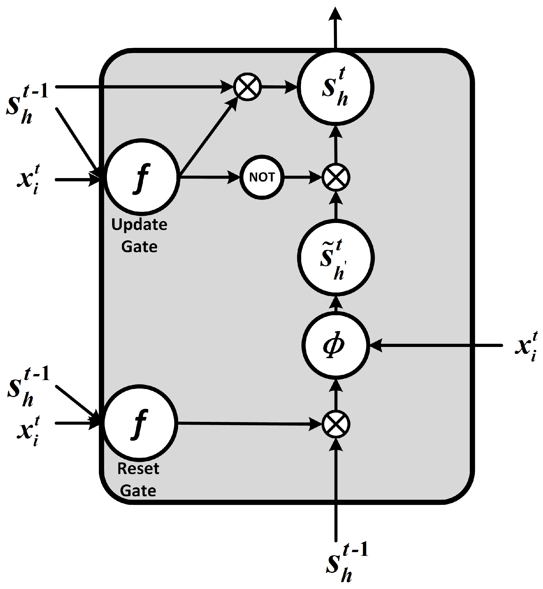
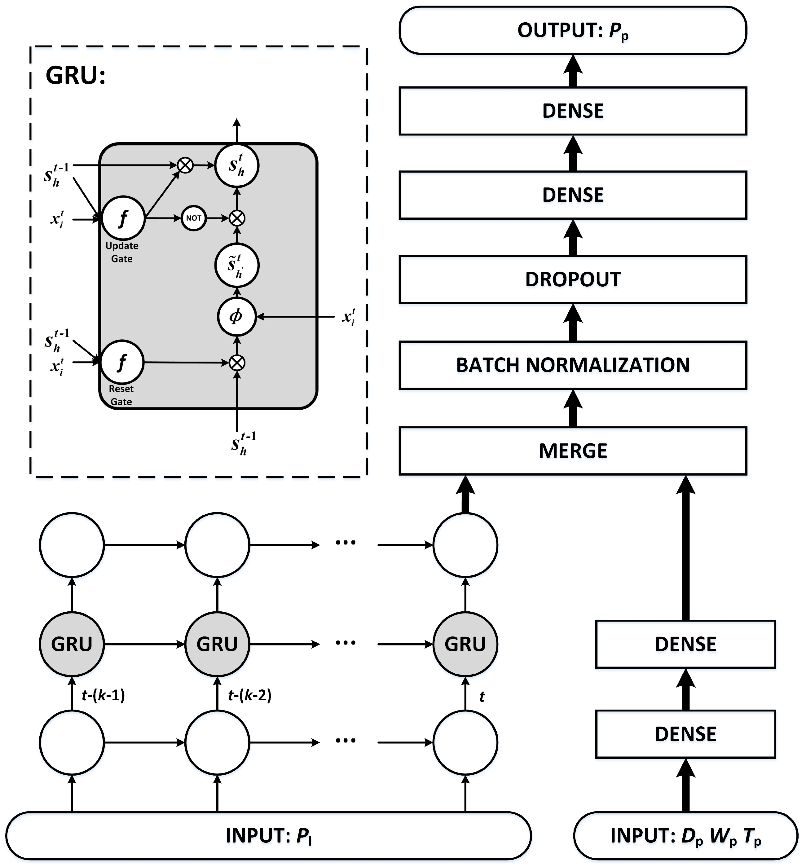
The vanishing gradient problem can be solved by adding control gates for remembering information in the process of data transfer. In LSTM networks, the hidden units of RNNs are replaced with LSTM blocks consisting of cell, input gate, output gate and forget gate. Moreover, the forget gate and input gate are combined into a single update gate in GRU neural network. The structure of GRU is shown in Figure 2.

The feedforward deduction process for GRU units is shown in Figure 2 and given by Equations (4)–(10).

$$a_u^t=\sum _{i=1}^I{w}_{iu}{x}_i^t+\sum _{h=1}^H{w}_{hu}{s}_h^{t-1}$$

(4)

$$s_u^t=f\left(a_u^t\right)$$

(5)

$$a_r^t=\sum _{i=1}^I{w}_{ir}{x}_i^t+\sum _{h=1}^H{w}_{hr}{s}_h^{t-1}$$

(6)

$$s_r^t=f\left(a_r^t\right)$$

(7)

$${\tilde{a}}_{h^{\prime }}^t=s_u^t\sum _{h=1}^H{w}_{h{h}^{\prime }}{s}_h^{t-1}+\sum _{i=1}^I{w}_{i{h}^{\prime }}{x}_i^t$$

(8)

$${\tilde{s}}_{h^{\prime }}^t=\varphi \left({\tilde{a}}_{h^{\prime }}^t\right)$$

(9)

$$s_h^t=(1-s_u^t){\tilde{s}}_{h^{\prime }}^t+s_u^t{s}_h^{t-1}$$

(10)

where u is the number of update gate vector; r is the number of reset gate vector; h is the number of hidden vectors at t time step; $h^{\prime }$ is the number of hidden vectors at $t-1$ time step; f and $\varphi$ are the activation functions; f is the sigmoid function and $\varphi$ is the tanh function generally; and ${\tilde{s}}_{h^{\prime }}^t$ means the new memory of hidden units at t time step.

According to Figure 2, the new memory ${\tilde{s}}_{h^{\prime }}^t$ is generated by the input $x_i^t$ at the current time step and the hidden unit state $s_h^{t-1}$ at the last time step, which means the new memory can combine the new information and the historical information. The reset gate determines the importance of $s_h^{t-1}$ to ${\tilde{s}}_{h^{\prime }}^t$. If the historical information $s_h^{t-1}$ is not related to new memory, the reset gate can completely eliminate the information in the past. The update gate determines the degree of transfer from $s_h^{t-1}$ to $s_h^t$. If $s_u^t\approx 1$, $s_h^{t-1}$ is almost completely passed to $s_h^t$. If $s_u^t\approx 0$, ${\tilde{s}}_{h^{\prime }}^t$ is passed to $s_h^t$. The structure shown in Figure 2 results in a long memory in GRU neural networks. The memory mechanism solves the vanishing gradient problem of original RNNs. Moreover, compared to LSTM networks, GRU neural networks merge the input gate and forget gate, and fuse the cell units and hidden units in LSTM block. It maintains the performance with simpler architecture, less parameters and less convergence time [33]. Correspondingly, GRU neural networks are trained by back-propagation through time as RNNs [35].

2.2. Data Description

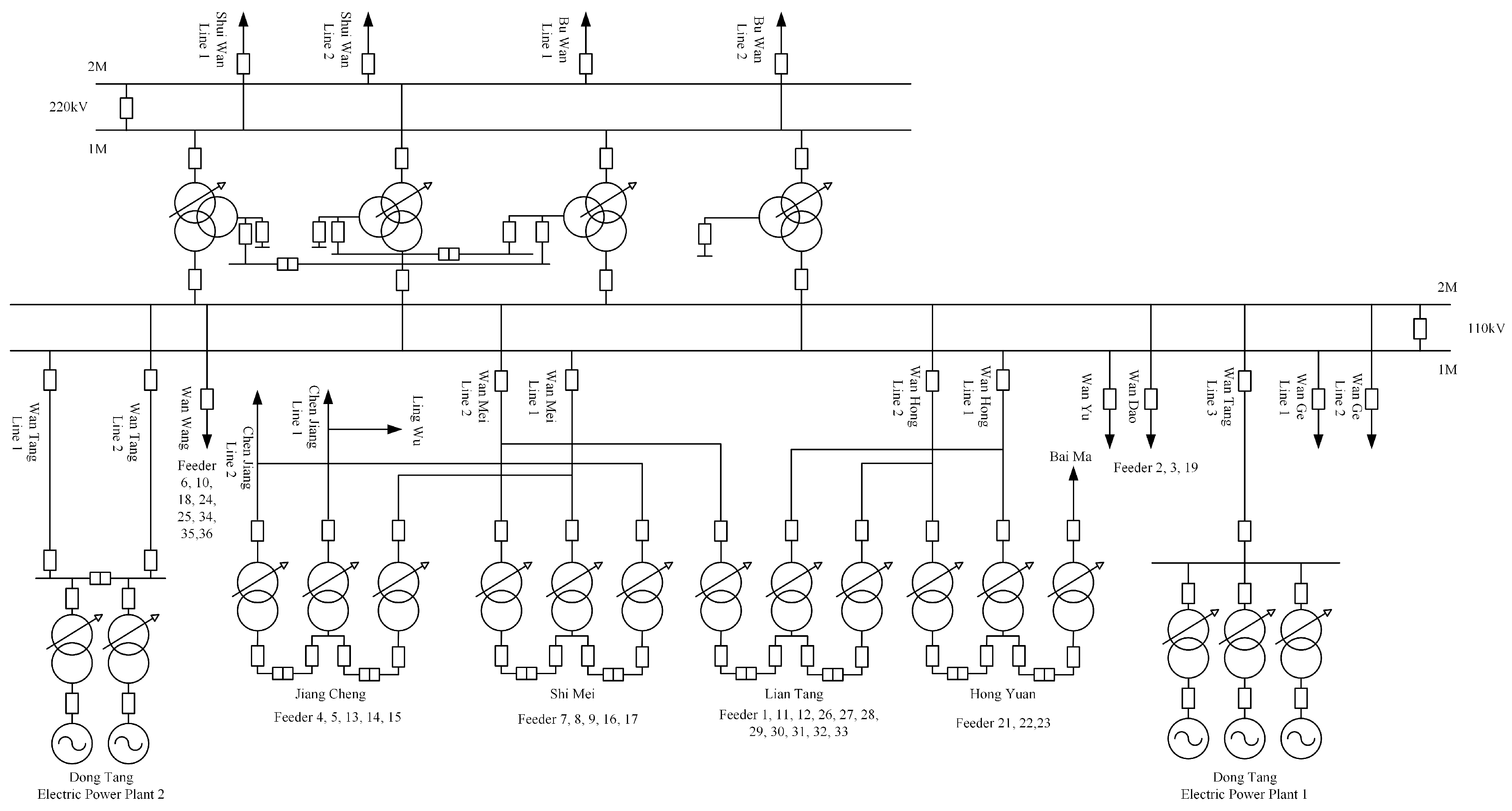
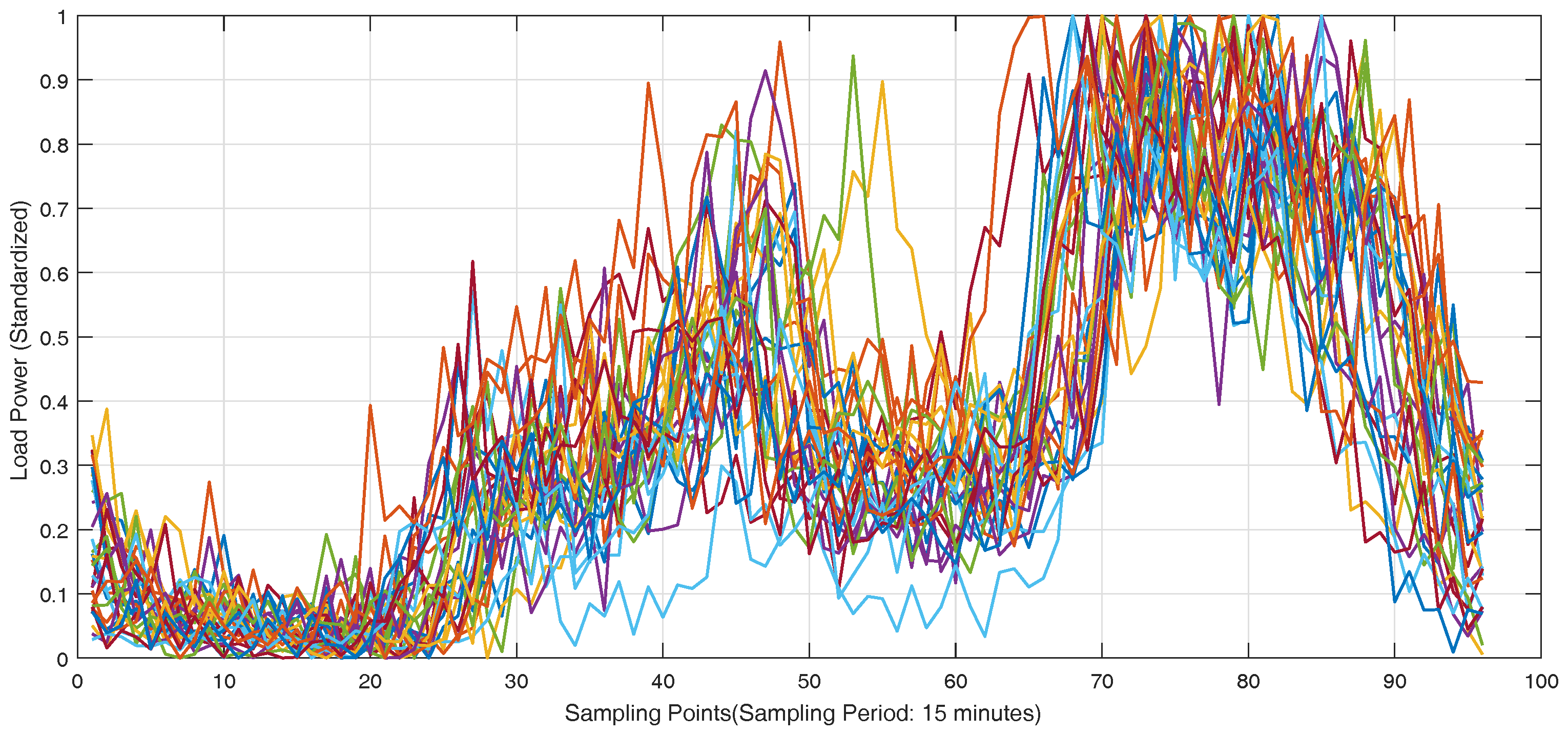
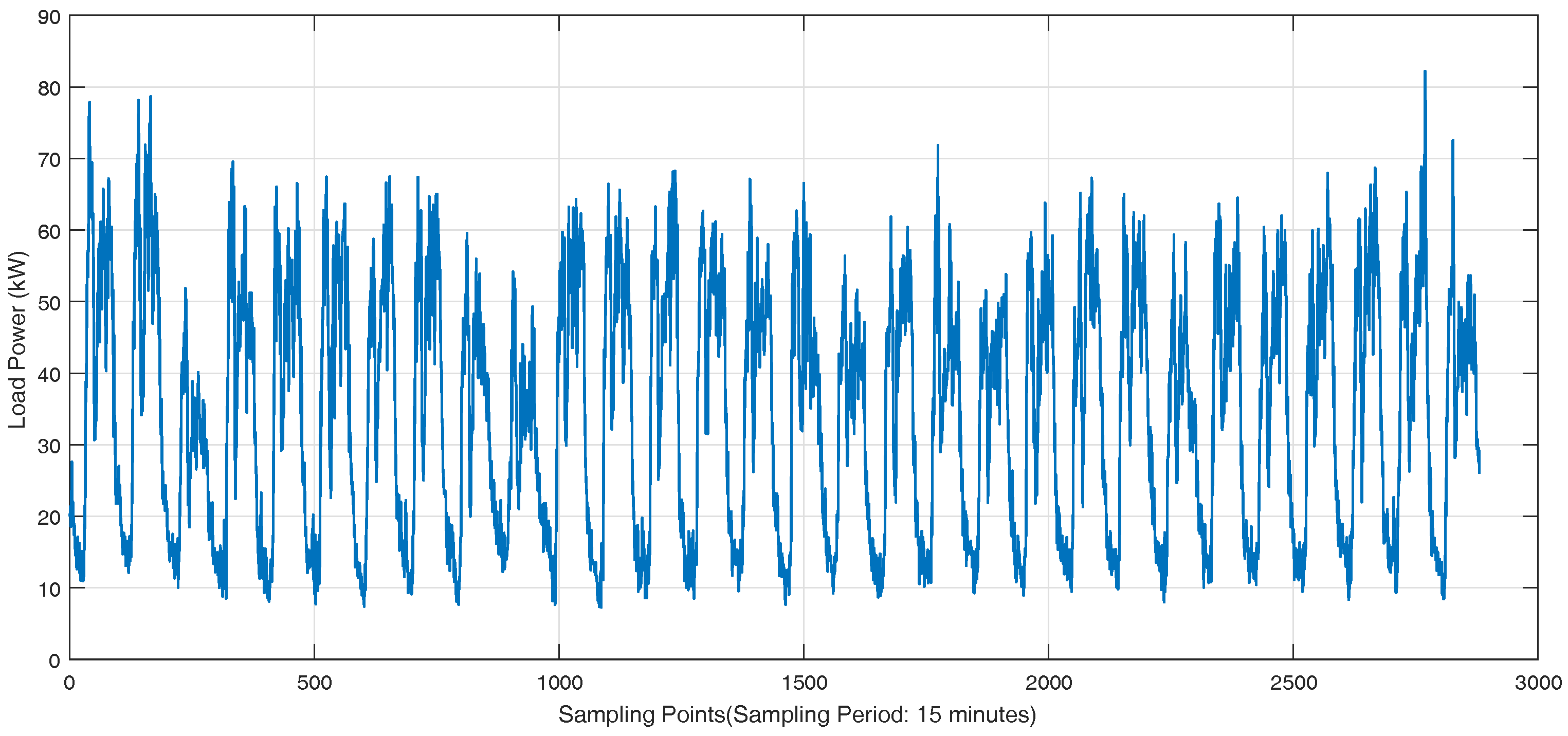
The real-world load data of individual customers in Wanjiang area is recorded from Dongguan Power Supply Bureau of China Southern Power Grid in Guangdong Province, China during 2012–2014. The topology structure of Wanjiang area is shown in Figure 3. There are 36 feeders connecting to the load sides in the Wanjiang area, i.e., Feeders 1—36. The active power is extracted for load forecasting from these feeders. The sampling period is 15 min as the meter record data. The load curve of a customer, No. 53990001, from Feeder 2 during a month is shown in Figure 4, where the different load characteristics of the customer on each day can be concluded.

Besides the historical load curves, short-term load forecasting is influenced by the factors of date, weather and temperature. The real historical data of weather and temperature in the corresponding area in Dongguan City were obtained online from the weather forecast websites. The categories of weather include sunny, cloud, overcast, light rain, shower, heavy rain, typhoon and snow. The date features can be found in calendars.

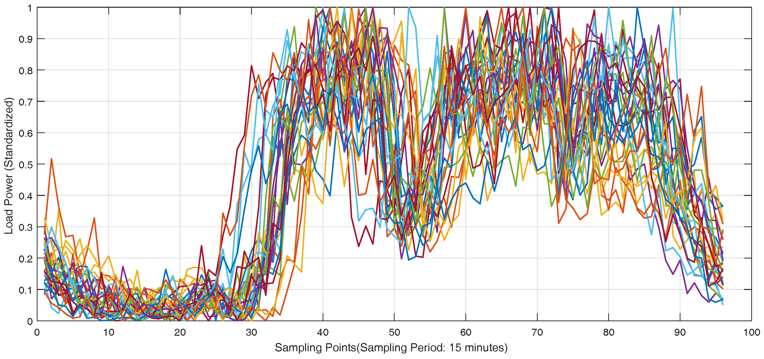
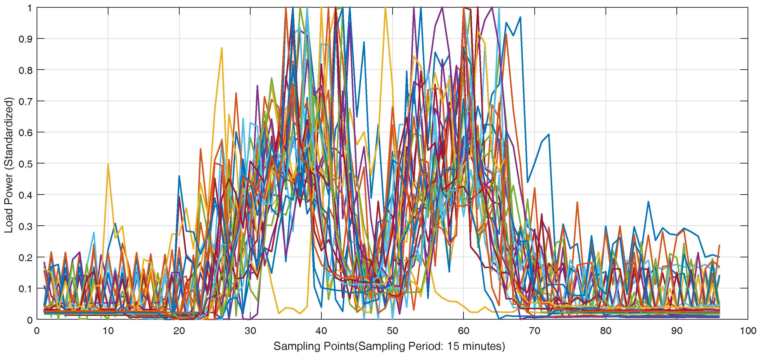
2.3. Clustering and Quantization

The custom of electricity use and characteristics of load curve are different among the different categories of customers such as industrial customers, residential customers and institution customers. The different characteristics would affect the performance of forecasting. Training forecasting networks with each customer separately would be a huge computation and storage problem. Therefore, in the proposed method, the load curve samples are divided into certain categories using K-means clustering algorithm. Samples with similar characteristics form a certain category, which form the input of GRU neural networks for the corresponding customers. K-means clustering algorithm is a simple and available method for clustering through unsupervised learning with fast convergence and less parameters. The only parameter, K, number of clustering category, can be determined by Elbow method with the turning point of loss function curve.

Suppose the input sample is $S=x_1,x_2,\dots ,x_m$. The algorithm is shown as follows.

• Randomly initialize K clustering centroids $c_1,c_2,\dots ,c_K$.
• For i = 1, 2, …, m, label each sample $x_i$ with the clustering centroid closest to $x_i$, getting K categories noted by $G_k$.

  $$labe{l}_i=\underset{1\le k\le K}{argmin}\parallel x_i-c_k\parallel ,i=1,2,\dots ,m$$

  (11)
• For k = 1, 2, …, K, average the samples assigned to $G_k$ to update $c_k$.

  $$c_k=\frac{1}{\left|G_k\right|}\sum _{i\in G_k}{x}_i,k=1,2,\dots ,K$$

  (12)
• Repeat Steps 2 and 3 until the change of clustering centroid or the loss function of clustering less than a set threshold. The loss function is given by Equation (13), where $x_j$ is the samples in categories $G_k$, $j=1,2,\dots ,n_k$ and $n_k$ is the number of samples in categories $G_k$.

  $$J(c_1,c_2,\dots ,c_K)=\frac{1}{2}\sum _{k=1}^K\sum _{j=1}^{n_k}\parallel x_j-c_k\parallel$$

  (13)

Moreover, the factors of date, weather and temperature should be added into input with quantization. First, the power consumption should be different between weekdays and weekends. The official holidays are also an important factor, so we quantify the date index as shown in

Table 1. Quantization for the factors of date.

Date (D)	Mon.	Tues.	Wed.	Thur.	Fri.	Sat.	Sun.	Official Holidays
Index	0	0.02	0.04	0.06	0.08	0.6	0.8	1

, where the index of official holidays is 1 no matter what day it is. Similarly, the weather and temperature are quantified according to their inner relations, as shown in

Table 2. Quantization for the factors of weather.

Weather (W)	Sunny	Cloud	Overcast	Light Rain	Shower	Heavy Rain	Typhoon	Snow
Index	0	0.1	0.2	0.4	0.5	0.6	0.8	1

and

Table 3. Quantization for the factors of temperature.

Temperature (T/°C)	T ≤ 0	0 < T ≤ 10	10 < T ≤ 20	20 < T ≤ 30	30 < T ≤ 40	T ≥ 40
Index	0	0.2	0.4	0.6	0.8	1

.

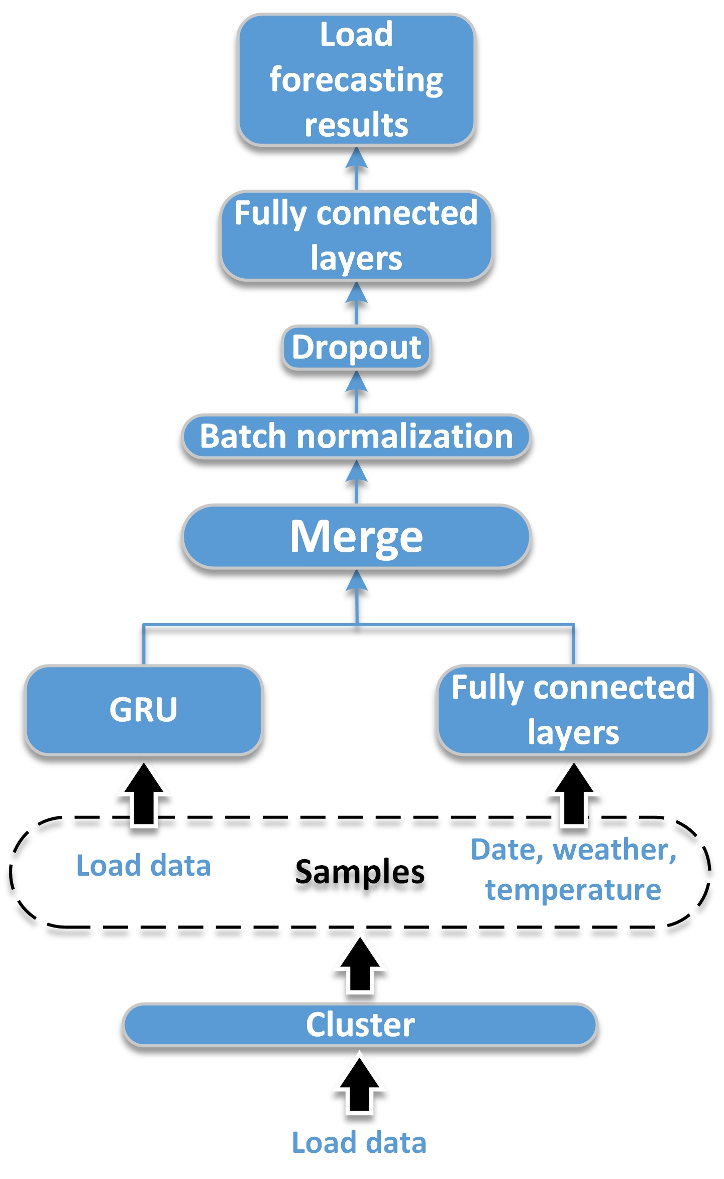
2.4. The Proposed Framework Based on GRU Neural Networks

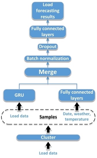
The schematic diagram of proposed framework based on GRU neural networks for short-term load forecasting is shown in Figure 5. The individual customers are clustered into a few categories for more accurate forecasting. The samples are recorded from the categories where the customer to be predicted locates in. The load measurement data of individual customers in one day is extracted as a sample for short-term load forecasting, noted by $\mathit{P}$. The dimension of $\mathit{P}$ is 96 with the 15 min sampling period. Then, the samples are reshaped into two-dimension for the input of GRU neural networks. Considering the influencing factors date $\mathit{D}$, weather $\mathit{W}$ and temperature $\mathit{T}$, date $D_{\mathrm{p}}$, weather $W_{\mathrm{p}}$ and temperature $T_{\mathrm{p}}$ on the forecasting day are added to the another input of the GRU neural networks. Considering the general factor of date, the prediction interval is set to seven days. Therefore, the load measurement data ${\mathit{P}}_{\mathrm{l}}$ on the day in the last week from the forecasting day, $D_{\mathrm{p}}$, $W_{\mathrm{p}}$ and $T_{\mathrm{p}}$, are recorded as the overall input. The load measurement data ${\mathit{P}}_{\mathrm{p}}$ on the forecasting day are recorded as the output, whose dimension is 96. Therefore, the input $\mathit{X}$ and output $\mathit{Y}$ of samples are given by Equations (14) and (15).

$$\mathit{X}=\{{\mathit{P}}_{\mathrm{l}};D_{\mathrm{p}},W_{\mathrm{p}},T_{\mathrm{p}}\}$$

(14)

$$\mathit{Y}=\left\{{\mathit{P}}_{\mathrm{p}}\right\}$$

(15)

The features from GRU neural networks and fully connected neural network are merged with the concatenating mode and passes through batch normalization and dropout layer to avoid overfitting and increase the learning efficiency. The principle is that batch normalization can avoid the gradient vanishing of falling into the saturated zone, and that the better performance in fixed combination is avoided when random neurons do not work in a dropout layer. Then, two-layer fully connected neural network are added before the output for learning and generalization ability. With training by back-propagation through time, the whole network implements the short-term load forecasting for individual customers. The structure can be extended if there is more information in the practical situation. The basic theory is also acceptable for medium-term load forecasting and long-term load forecasting, but different influence factors should be considered and the model should be changed with different input, output, and inner structure for good performance.

3. Experiments and Results

In this section, the experiments are described in detail and the results are shown in figures and tables. The specific discussion for results is elaborated after the results and prove the improved performance compared to other methods. The data for experiments are recorded in Section 2.2.

3.1. Clustering Analysis for Load Curve of Individual Customers

Before the short-term load forecasting using GRU neural networks, the load curves of individual customers are clustered to different categories for samples with K-means clustering algorithm. The parameter K is selected as 3 by Elbow method. There are 746 customers in the Wanjiang area in Dongguan city. The load measurement data should be processed with 0–1 standardization to the same scale for clustering to reduce the impact of different magnitudes and dimensions. The clustering is done for 10 times with load curves in 10 days for the individual customers. The clustering results are obtained with the average results in 10 days and the number of each clustering category is shown in

Table 4. Number of each clustering category.

Categories	Category 1	Category 2	Category 3
Number of Customers	221	308	217

. The standardized curves for 30 selected customers in three categories on a weekday are shown in Figure 6, Figure 7 and Figure 8.

As can be seen in Figure 6, Figure 7 and Figure 8, different customers have different characteristics of electricity use. According to Figure 6, there are two electric peaks in a day. The evening peak is higher than the noon peak. The classic representation of this characteristic in Figure 6 is residential customers. Different from Figure 6, Figure 7 maintains the peak from 9 a.m. to late at night except noon. They are the general load curves of industry and business customers. In Figure 8, there are two electric peaks in the morning and afternoon. It should belong to the government and institutional customers. Even though a few customers have differences with the overall curve, this is the best clustering for them and it does not influence the overall performance greatly. With the clustering of individual customers, the networks can be trained with samples in the same category according to the customer to be predicted, so that the interference of electricity use characteristics can be reduced.

3.2. The Detailed Network Structure and Parameters

The detailed structure of whole network are shown in

Table 5. Number of units in the proposed network.

Layer	Number of Units	Layer	Number of Units
INPUT: $P_{\mathrm{l}}$	(6, 16)	INPUT: $D_p$ $W_p$ $T_p$	3
BATCH NORMALIZATION	(6, 16)	DENSE1	100
GRU	300	DENSE2	100
MERGE	400
DROPOUT	400
DENSE3	100
DENSE4	100
OUTPUT:$P_{\mathrm{p}}$	96

. The parameters of the network are set as shown in

Table 6. Parameter setting in the proposed network.

Parameters	Value
Input Time Steps	6
Input Dimension	16
Batch Size	30
Epoch	200
Optimizer	RMSprop
Learning Rate	0.001
Decay	0.9
Dropout Rate	0.6

. The structure and parameters are set for better performance according to the multiple experiments for customers in Wanjiang area. The “RMSprop” optimizer is chosen for its better performance in recurrent neural networks. The parameters can be adjusted for the different practical situations. In this paper, the number of epoch is set to 200 for the proposed method and can be adjusted for the compared methods. The training is stopped when the error decreases to a steady state.

3.3. Comparison of Results of Proposed Method

The results of the proposed method are shown as follows. In the experiments, the training samples are recorded from the load data in the period from October 2012 to September 2013 while the test samples are recorded from load data in the period from October to December of 2013. The number of recorded training samples and test samples of each categories is 36,000 and 9000, respectively, with 100 customers in a category. The ratio of sample number is 4:1. Mean absolute percentage error (MAPE) is the classic evaluation index for load forecasting. The computational formula is given by Equations (16) and (17), where $n=96$ represents the dimension of samples and m represents the number of test samples.

$$MAPE=\frac{{\sum }_{j=1}^m\left|E_j\right|}{m}\times 100\%$$

(16)

$$E_j=\frac{{\sum }_{i=1}^n\left|P_{\mathrm{p},\mathrm{ij}}-P_{\mathrm{l},\mathrm{ij}}\right|}{n}$$

(17)

Customer 53990001 is selected from Category 2 for the forecasting customer. The MAPEs during a training period for Category 2 are shown in Figure 9 when the parameters are set as shown in Table 6. The compared curves of actual load and forecasting load using the proposed method on 18 November for Customer 53990001 are shown in Figure 10. The MAPE for Customer 53990001 on 18 November is 10.23%. The compared curves of actual load and forecasting load from 18 to 24 November for Customer 53990001 are shown in Figure 11. The MAPE for Customer 53990001 in this week is 10.97%. In Figure 10 and Figure 11, the error in sample points of one day is basically average and becomes larger when the curve comes to a peak. It is reasonable because the high or low peak is not reachable in most cases. The network should balance the prediction results for most situations during the training process. According to Figure 9, the MAPE decreases to a steady state as the epoch increases to 200. According to Figure 10 and Figure 11, the forecasting curve is close to the actual curve, which proves the availability of the proposed method.

The samples are preprocessed by K-means clustering algorithm to form three categories for training. We performed a comparative experiment with variable-controlling approach about clustering. The compared results of Customer 53990001 on four different days of November 2013 are shown in Figure 12. The compared MAPEs of prediction on 18 November for nine customers in three categories from different feeders are shown in

Table 7. Compared MAPEs for nine customers in three categories with or without clustering.

Customer	Category	Feeder	MAPE with Clustering	MAPE without Clustering
37148000	1	2	10.80%	22.98%
51690000	1	7	9.25%	21.17%
37165000	1	7	11.12%	20.12%
53990001	2	2	10.07%	27.31%
54265001	2	3	11.91%	22.72%
54265002	2	3	10.76%	28.45%
31624001	3	35	13.56%	21.12%
41661001	3	34	12.23%	24.85%
76242001	3	33	9.98%	28.38%

. It can be concluded that the forecasting curve without clustering deviates from the actual curve and that its MAPE is larger. The reason is that different characteristics of electricity use create a bad effect for short-term load forecasting. The effect reduces when we use corresponding trained networks for different customers. Therefore, the performance is generally improved by clustering.

The input of proposed network includes $D_{\mathrm{p}}$, $W_{\mathrm{p}}$, $T_{\mathrm{p}}$ and ${\mathit{P}}_{\mathrm{l}}$, which means that the network obtains and fuses the previous load changing process and other environmental information. In this case, we removed the input layer and the following fully connected layers in the network. The comparison results of Customer 53990001 with multi-source or only load data input are shown in Figure 13. The compared MAPEs for nine customers in three categories from different feeders are shown in

Table 8. Compared MAPEs for nine customers in three categories with multi-source data or only load data.

Customer	Category	Feeder	MAPE with Multi-Source Data	MAPE with only Load Data
37148000	1	2	10.80%	15.09%
51690000	1	7	9.25%	15.06%
37165000	1	7	11.12%	16.50%
53990001	2	2	10.07%	18.56%
54265001	2	3	11.91%	17.36%
54265002	2	3	10.76%	15.99%
31624001	3	35	13.56%	15.89%
41661001	3	34	12.23%	16.46%
76242001	3	33	9.98%	17.33%

. The experimental condition is the same as the one above. It can be concluded that the performance of only using load data is obviously poorer. Although the change shape is similar to actual, the curves deviate from the actual curves. Correspondingly, the MAPEs are larger. The reason is that date, weather and temperature are necessary factors to consider during short-term load forecasting processing. People would raise their load on a hot or cold day, even a rainy or snowy day. Resident customers may increase electricity consumption on weekends but business customers may not. These are some obvious reasons why we should consider the environment factors.

It can be concluded from the two experiments that the MAPEs are floating in a certain degree. The maximal MAPEs of all samples in the conditions of the two experiments are shown in

Table 9. Maximal MAPEs in different conditions.

Conditions	Forecast without Clustering	Forecast with only Load Data	Proposed Method
Maximal MAPE	30.25%	21.87%	15.12%

. The maximal MAPE without clustering and with only load data is significantly larger than the proposed method with clustering and multi-source data. The maximal MAPE of proposed method is 15.12%, which is acceptable for load forecasting of individual customers.

The performances are good with LSTM networks in dealing with time sequence but there are more parameters to train compared with GRU neural networks. In the proposed network, the GRU layers have 285,300 parameters to train while the LSTM layers have 380,400 parameters with the same architecture. The cost time for training with LSTM network is about 20% longer than training with GRU neural networks in the experiments in this paper. The MAPEs of network with LSTM and GRU layer in the same architecture with the same samples in Category 2 during the training process are shown in Figure 14. We can conclude that GRU neural networks do better in both convergence speed and training time, which depends on the improved single structure of GRU units.

We also performed the experiments to compare with current methods such as back-propagation neural networks (BPNNs) [7,8], stacked autoencoders (SAEs) [17], RNNs [24,25], and LSTM [29,30,31]. Their parameters and structures are set as described in Section 3.2. The compared average MAPEs of these methods, trained and tested with all samples described at the beginning of this subsection, are shown in Figure 15. The specific values of average and maximal MAPEs are shown in

Table 10. Average and maximal MAPEs of the proposed and current methods for short-term load forecasting.

Method	BPNNs	SAEs	RNNs	LSTM	Proposed Method
Average MAPE	26.12%	23.23%	16.85%	13.26%	10.98%
Maximal MAPE	32.42%	28.51%	20.97%	17.45%	15.12%

. Moreover, the results of nine customers are shown to validate the better performance of the proposed methods. The MAPEs for 30 November 2013 are shown in

Table 11. MAPEs of compared methods for nine customers’ short-term load forecasting on 30 November 2013.

Customer	Category	Feeder	BPNNs	SAEs	RNNs	LSTM	Proposed Method
37148000	1	2	26.96%	23.28%	16.56%	13.09%	10.80%
51690000	1	7	27.56%	25.61%	15.56%	10.77%	9.25%
37165000	1	7	28.55%	24.81%	13.35%	14.55%	11.12%
53990001	2	2	24.23%	22.23%	17.87%	11.27%	10.07%
54265001	2	3	26.33%	27.56%	17.23%	12.22%	11.91%
54265002	2	3	29.23%	24.89%	15.63%	14.63%	10.76%
31624001	3	35	30.45%	22.56%	19.93%	12.29%	13.56%
41661001	3	34	32.23%	25.65%	16.72%	14.65%	12.23%
76242001	3	33	25.36%	23.22%	14.66%	13.27%	9.98%

. It can be concluded that the proposed method results in smaller error in both average and maximal MAPEs. The proposed method performs better compared to the other current methods in most cases for short-term load forecasting in Wanjiang area.

In detail, the forecasting load curves of Customers 37148000 and 53990001 on 30 November 2013 based on these methods are shown in Figure 16 and Figure 17. We can observe the closest curve to the actual curve is the proposed method in the results of these experiments. Time information is important in short-term load forecasting which the BPNNs and SAEs cannot extract. Therefore, they get poorer performance in the experiments. The vanishing gradient problem limits the performance of RNNs because of the decreasing perception of nodes. The architecture is simpler and the parameters are fewer in GRU neural network compared to LSTM networks (Section 2.1). Therefore, the performances of GRU neural networks are better than the other current methods. In general, the availability and improvement of the proposed method are proven by the real-world experiments.

4. Conclusions

To increase the stability and economy of power grids, a method for short-term load forecasting with multi-source data using GRU neural networks is proposed in this paper, which focuses on individual customers. The proposed structure of the whole network is shown in Figure 5. The real-world load data of individual customers is recorded from Dongguan Power Supply Bureau of China Southern Power Grid in Guangdong Province, China. Before training, the customers with load data are clustered into three categories by K-means clustering algorithm to reduce the interference of different electricity use characteristics. Then, the environment factors are quantified and put into the input of the proposed networks for more information. The GRU units are introduced into the network for its simpler structure and faster convergence compared to LSTM blocks. The results in Figure 12 and Figure 13 show that clustering and multi-source input can help to improve the performance of load forecasting. The average MAPE can be low as 10.98% for the proposed method, which outperforms the other current methods such as BPNNs, SAEs, RNNs and LSTM. The improvement is notable (Figure 15, Figure 16 and Figure 17). In general, the availability and superiority of the proposed method are verified in this paper. In the future, combining with the technique of peak prediction could be a subject worth studying for load forecasting. Moreover, since the load forecasting for the customers in all power grid areas is a large-scale task, transfer learning and continuous learning will be considered based on the proposed framework for high-efficiency load forecasting.

References

1. Espinoza, M.; Suykens, J.A.; Belmans, R.; De Moor, B. Electric load forecasting. IEEE Contr. Syst. Mag. 2007, 27, 43–57. [Google Scholar] [CrossRef]
2. Hong, T. Energy forecasting: Past, present, and future. Foresight Int. J. Appl. Forecast. 2014, 32, 43–48. [Google Scholar]
3. Gross, G.; Galiana, F.D. Short-term load forecasting. Proc. IEEE 1987, 75, 1558–1573. [Google Scholar] [CrossRef]
4. Hong, T.; Fan, S. Probabilistic electric load forecasting: A tutorial review. Int. J. Forecast. 2016, 32, 914–938. [Google Scholar] [CrossRef]
5. Taylor, J.W.; McSharry, P.E. Short-term load forecasting methods: An evaluation based on european data. IEEE Trans. Power Syst. 2008, 22, 2213–2219. [Google Scholar] [CrossRef]
6. Chen, H.; Wan, Q.; Zhang, B.; Li, F.; Wang, Y. Short-term load forecasting based on asymmetric ARCH models. In Proceedings of the Power and Energy Society General Meeting, Providence, RI, USA, 25–29 July 2010; pp. 1–6. [Google Scholar]
7. Quan, H.; Srinivasan, D.; Khosravi, A. Short-term load and wind power forecasting using neural network-based prediction intervals. IEEE Trans. Neural Netw. Learn. Syst. 2014, 22, 303–315. [Google Scholar] [CrossRef] [PubMed]
8. Ding, N.; Benoit, C.; Foggia, G.; Besanger, Y.; Wurtz, F. Neural network-based model design for short-term load forecast in distribution systems. IEEE Trans. Power Syst. 2016, 31, 72–81. [Google Scholar] [CrossRef]
9. Cevik, H.H.; CunkaS, M. Short-term load forecasting using fuzzy logic and ANFIS. Neural Comput. Appl. 2015, 26, 1355–1367. [Google Scholar] [CrossRef]
10. Lee, C.W.; Lin, B.Y. Applications of the chaotic quantum genetic algorithm with support vector regression in load forecasting. Energies 2017, 10, 1832. [Google Scholar] [CrossRef]
11. Hinton, G.E.; Salakhutdinov, R.R. Reducing the dimensionality of data with neural networks. Science 2006, 313, 504–507. [Google Scholar] [CrossRef] [PubMed]
12. Hinton, G.E.; Osindero, S.; Teh, Y.W. A fast learning algorithm for deep belief nets. Neural Comput. 2006, 18, 1527–1554. [Google Scholar] [CrossRef] [PubMed]
13. Chen, K.; Huang, C.; He, J. Fault detection, classification and location for transmission lines and distribution systems: A review on the methods. High Volt. 2016, 1, 25–33. [Google Scholar] [CrossRef]
14. Wang, Y.; Liu, M.; Bao, Z. Deep learning neural network for power system fault diagnosis. In Proceedings of the 35th Chinese Control Conference, Chengdu, China, 27–29 July 2016; pp. 6678–6683. [Google Scholar]
15. Ryu, S.; Noh, J.; Kim, H. Deep neural network based demand side short term load forecasting. Energies 2016, 10, 3. [Google Scholar] [CrossRef]
16. Qiu, X.; Ren, Y.; Suganthan, P.N.; Amaratunga, G.A. Empirical mode decomposition based ensemble deep learning for load demand time series forecasting. Appl. Soft Comput. 2017, 54, 246–255. [Google Scholar] [CrossRef]
17. Tong, C.; Li, J.; Lang, C.; Kong, F.; Niu, J.; Rodrigues, J.J. An efficient deep model for day-ahead electricity load forecasting with stacked denoising auto-encoders. J. Parallel Distrib. Comput. 2017, 1–7. [Google Scholar] [CrossRef]
18. Liao, Y.; Chen, S. A modular RNN-based method for continuous Mandarin speech recognition. IEEE Trans. Speech Aud. Proc. 2016, 9, 252–263. [Google Scholar] [CrossRef]
19. Nakashika, T.; Takiguchi, T.; Ariki, Y. Voice conversion using RNN pre-trained by recurrent temporal restricted Boltzmann machines. IEEE/ACM Trans. Aud. Speech Lang. Proc. 2015, 23, 580–587. [Google Scholar] [CrossRef]
20. Wu, H.; Prasad, S. Convolutional recurrent neural networks forhyperspectral data classification. Remote Sens. 2017, 9, 298. [Google Scholar] [CrossRef]
21. Zuo, H.; Fan, H.; Blasch, E.; Ling, H. Combining convolutional and recurrent neural networks for human skin detection. IEEE Signal Proc. Lett. 2017, 24, 289–293. [Google Scholar] [CrossRef]
22. Chien, J.T.; Ku, Y.C. Bayesian recurrent neural network for language modeling. IEEE Trans. Neural Netw. Learn. Syst. 2016, 27, 361–374. [Google Scholar] [CrossRef] [PubMed]
23. Ororbia, A.G., II; Mikolov, T.; Reitter, D. Learning simpler language models with the differential state framework. Neural Comput. 2017, 29, 3327–3352. [Google Scholar] [CrossRef] [PubMed]
24. Shi, H.; Xu, M.; Li, R. Deep learning for household load forecasting—A novel pooling deep RNN. IEEE Trans. Smart Grid 2017, 1–10. [Google Scholar] [CrossRef]
25. Wei, L.Y.; Tsai, C.H.; Chung, Y.C.; Liao, K.H.; Chueh, H.E.; Lin, J.S. A study of the hybrid recurrent neural network model for electricity loads forecasting. Int. J. Acad. Res. Account. Fin. Manag. Sci. 2017, 7, 21–29. [Google Scholar]
26. Hochreiter, S.; Schmidhuber, J. Long short-term memory. Neural Comput. 1997, 9, 1735–1780. [Google Scholar] [CrossRef] [PubMed]
27. Wei, D.; Wang, B.; Lin, G.; Liu, D.; Dong, Z.; Liu, H.; Liu, Y. Research on unstructured text data mining and fault classification based on RNN-LSTM with malfunction inspection report. Energies 2017, 10, 406. [Google Scholar] [CrossRef]
28. Zhang, S.; Wang, Y.; Liu, M.; Bao, Z. Data-based line trip fault prediction in power systems using LSTM networks and SVM. IEEE Access 2017, 6, 7675–7686. [Google Scholar] [CrossRef]
29. Gensler, A.; Henze, J.; Sick, B.; Raabe, N. Deep Learning for solar power forecasting—An approach using AutoEncoder and LSTM Neural Networks. In Proceedings of the International Conference on Systems, Man, and Cybernetics, Budapest, Hungary, 9–12 October 2016; pp. 2858–2865. [Google Scholar]
30. Zheng, J.; Xu, C.; Zhang, Z.; Li, X. Electric load forecasting in smart grids using long-short-term-memory based recurrent neural network. In Proceedings of the 51st Annual Conference on Information Sciences and Systems, Baltimore, MD, USA, 22–24 March 2017; pp. 1–6. [Google Scholar]
31. Kong, W.; Dong, Z.Y.; Jia, Y.; Hill, D.J.; Xu, Y.; Zhang, Y. Short-term residential load forecasting based on LSTM recurrent neural network. IEEE Trans. Smart Grid 2017, 1–11. [Google Scholar] [CrossRef]
32. Cho, K.; Van Merrienboer, B.; Gulcehre, C.; Bahdanau, D.; Bougares, F.; Schwenk, H.; Bengio, Y. Learning phrase representations using RNN encoder-decoder for statistical machine translation. arXiv, 2014; arXiv:1406.1078. [Google Scholar]
33. Chung, J.; Gulcehre, C.; Cho, K.; Bengio, Y. Empirical evaluation of gated recurrent neural networks on sequence modeling. arXiv, 2014; arXiv:1412.3555. [Google Scholar]
34. Lu, K.; Zhao, Y.; Wang, X.; Cheng, Y.; Pang, X.; Sun, W.; Jiang, Z.; Zhang, Y.; Xu, N.; Zhao, X. Short-term electricity load forecasting method based on multilayered self-normalizing GRU network. In Proceedings of the Conference on Energy Internet and Energy System Integration, Beijing, China, 26–28 November 2017; pp. 1–5. [Google Scholar]
35. Werbos, P.J. Backpropagation through time: What it does and how to do it. Proc. IEEE 1990, 78, 1550–1560. [Google Scholar] [CrossRef]
Figure 1. A simple RNN structure, where X is the input unit, H is the hidden unit, Y is the output unit, and W is the weight matrix.
Energies 11 01138 g001
Figure 2. Inner structure of GRU, where all arrows represent the weights between gates and units and the units of f and ϕ are the activation functions. The parameters are explained in detail after the Equations (4)–(10).
Energies 11 01138 g002
Figure 3. Primary electrical system in Wanjiang area above 110 kv, including electric power plants, transmission buses, converting stations, and user loads. The feeders are marked under their corresponding load sides.
Energies 11 01138 g003
Figure 4. Load curve of Customer 53990001 from Feeder 2 during a month, where the sampling period is 15 min.
Energies 11 01138 g004
Figure 5. Schematic diagram of proposed framework based on GRU Neural Networks for short-term load forecasting, where k is the number of hidden units and t is the time step. The parameters of GRU units are clarified in Section 2.1. The input and output parameters are explained in the next subsection.
Energies 11 01138 g005
Figure 6. Load curves of 30 customers in Category 1.
Energies 11 01138 g006
Figure 7. Load curves of 30 customers in Category 2.
Energies 11 01138 g007
Figure 8. Load curves of 30 customers in Category 3.
Energies 11 01138 g008
Figure 9. MAPEs during a training period for the Category 2.
Energies 11 01138 g009
Figure 10. Compared curves of actual load and forecasting load in a day for Customer 53990001.
Energies 11 01138 g010
Figure 11. Compared curves of actual load and forecasting load in a week for Customer 53990001.
Energies 11 01138 g011
Figure 12. Compared curves of actual load and forecasting load of Customer 53990001 with or without clustering: (ad) the results for four different days in November 2013.
Energies 11 01138 g012
Figure 13. Comparison curve of actual load and forecasting load of Customer 53990001 with or without multi-source data: (ad) the results for the same four days in November 2013 as the experiment in Figure 12.
Energies 11 01138 g013
Figure 14. The MAPEs of network with LSTM and GRU layers in the same architecture with same samples during the training process.
Energies 11 01138 g014
Figure 15. Compared average MAPEs trained and tested with all samples in three categories.
Energies 11 01138 g015
Figure 16. The load curves of Customer 37148000 based on the proposed method and the other current methods.
Energies 11 01138 g016
Figure 17. The load curves of Customer 53990001 based on the proposed method and the other current methods.
Energies 11 01138 g017