Abstract
The Colorado River is an important natural resource for the Southwestern United States. Predicted climate change impacts include increased temperature, decreased rainfall and increased probability of drought in this region. Given the large amount of hydropower on the Colorado River and its importance to the bulk electricity system, this purpose of this study was to quantify the value hydropower in operating the electrical system, and examined changes in hydropower value and electricity costs under different possible future drought conditions and regional generation scenarios. The goal was to better understand how these scenarios affect operating costs of the bulk electrical system, as well as the value of the hydropower produced, and proposed a method for doing so. The calculated value of the hydroelectric power was nearly double the mean locational marginal price in the study area, about $73 to $75 for most scenarios, demonstrating a high value of the hydropower. In general, it was found that reduced water availability increased operating costs, and increased the value of the hydropower. A calculated value factor showed that when less hydroelectric power is available, the hydropower is more valuable. Furthermore, the value factor showed that the value of hydro increases with the addition of solar or the retirement of thermal generating resources.
1. Introduction
Resource changes in the electricity sector are common and happen for many reasons. Prominent among these are changes in the cost of generation, such as the decrease in the cost of natural gas fired generation in the United States due to an increase in supply and increased plant efficiency [1], and the continuing decline in cost of wind and solar power [2,3,4]. Alternatively, there may be a shortage of a resource, for example, hydropower in California during the recent drought. It was estimated that hydropower production across the state was reduced by 57,000 GWh between 2012–2015 [5]. In the Southwestern (SW) United States, (Arizona, New Mexico, and parts of surrounding states) coal-fired power generation is being retired while more solar photovoltaic generation is being added, due to Renewable Energy Standards (RES) [6] and low costs [3]. Two examples of coal retirements are the Navajo Generating Station (NGS) in Page, Arizona, a 2250 MW coal generating plant, and the San Juan Generating Station in New Mexico, a 1,848 MW coal generating plant. Currently, the plan is to shut down NGS completely in December 2019 [7], while two units at San Juan will be decommissioned in December 2017, and the remaining two shut down in 2022 [8]. NGS provides power to four Southwest utilities, Salt River Project (SRP), Arizona Public Service (APS), NV Energy, and Tucson Electric Power (TEP), in addition to the federal share, which is 24.3% (547 MW) of the total plant capacity, and is used for loads associated with the U.S. Bureau of Reclamation, such as pumping loads for water conveyance. Part of the rationale for retiring NGS was that during a recent year, electricity from NGS cost about $38/MWh, but could be bought on the market for $32/MWh [9].
The current trends in electricity in the SW U.S. are creating new opportunities and challenges. The increasing amount of solar on the system creates the “duck curve”, particularly during the spring months, where midday net load is low, followed by a steep afternoon ramp when solar generation is decreasing and load is increasing [10]. Loads in the SW U.S. are driven largely by air conditioning, and as a result, are significantly lower during the non-summer months. Variability can be a problem with wind and solar. Many studies have examined the effects of increasing the amount of renewable energy on the grid [11,12,13,14,15,16], and all of those conclude that wind and solar power resources increase the variability of the net load (i.e., load minus wind and solar power generation) that must be served by the remaining generation fleet. Hydro has been found to be well suited to balance changes in net load due to renewables, because of its fast ramping and storage capabilities [17,18,19]. In some cases, however, hydro can be constrained by other factors, such as recreation downriver, and wildlife concerns, which reduce its ability to respond in a timely manner to electricity demands.
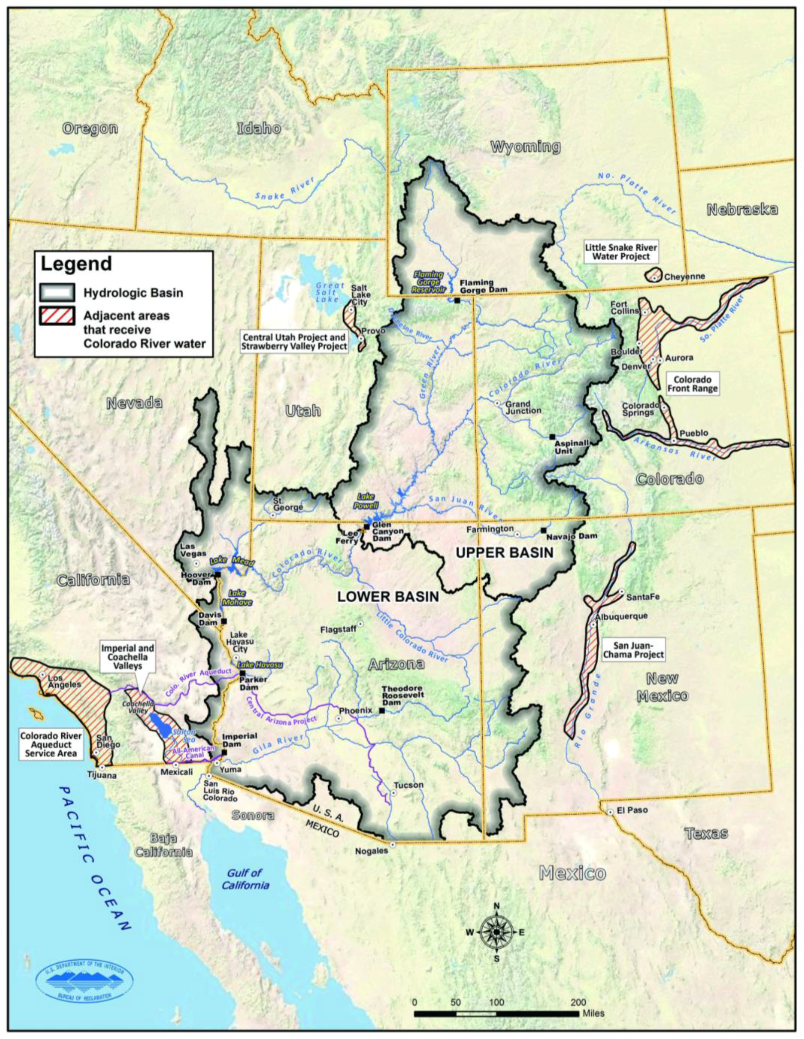
In the SW U.S., the major hydropower resource is the Colorado River. It has been called the “single most important natural resource in the Southwest” U.S., since 27 million people rely on it for drinking water and irrigation for 3.5 million acres of farmland [20]. The Colorado River Basin covers portions of seven U.S. states: California, Arizona, Nevada, Wyoming, Colorado, New Mexico, and Utah, as shown in Figure 1. There are nine hydropower dams in the Colorado River Basin owned and operated by the United States Bureau of Reclamation (Reclamation): Hoover, Glen Canyon, Davis, Parker, Blue Mesa, Crystal, Flaming Gorge, Morrow Point, and Fontenelle. Table 1 provides information about each dam, including reservoir name, water storage, generation capacity, and average annual electricity production. Together, these dams produce an average 10,000 gigawatt-hours (GWh) of electricity annually; the majority of this production comes from Hoover and Glen Canyon Dams with about 3800 GWh and 3700 GWh per year, respectively [21]. On the whole, the dams produce much more electricity in the summer when demand for downstream water delivery is high, as is the electricity demand. Some of the power plants in these dams, in general, have the ability to provide “ancillary services” to the electrical system; they can be ramped up or down quickly, and they typically have extra capacity available as reserves. The electricity available from any hydroelectric power plant is dependent upon its water releases and reservoir elevation. For its dams on the Colorado River, Reclamation creates an annual projection of month-to-month water releases and pool elevations based upon expected deliveries to its water customers. From these projections, an estimated power production schedule from each of its projects is created (e.g., maximum power available and monthly energy quota).

Figure 1.
Map of Colorado River Basin showing the major hydroelectric dams [23].

Table 1.
Major hydroelectric dams on the Colorado River System, including location, amount of water storage, installed capacity, and electricity production [21,22].
The Colorado River has historically had a wide variation in flow. Flows into Lake Powell, the Glen Canyon reservoir, are a good proxy for overall flow in the river, and Glen Canyon Dam generation is reflective of those inflows. Between 1980 and 2013, generation varied by a factor of 2.6, from a low of 3299 GWh in 2005 to a high of 8703 GWh in 1984 [24]. Due to climate change, the Southwestern United States is more likely to see high temperatures for longer periods of time, as well as decreased precipitation and larger probability of sustained drought [25]. The dams protect the region’s water supply from a certain amount of yearly variation, since they serve as large water storage facilities. However, the danger is in drought several years in a row, where the reservoirs are drawn down. As seen in Table 1, together Lake Powell and Lake Mead have over 60 cubic kilometers (km3) of water storage. The average annual flow for the Colorado River is about 18 km3 [23], and thus, there is more than 3 years’ worth of water stored in Lake Powell and Lake Mead.
According to the Annual Operating Plan for Colorado River Reservoirs 2015, “inflow to Lake Powell has been below average in 12 of the last 15 water years” [26]. (Note: Water years run from October 1 through September 30.) The period from 2000−2014 has been the driest period for the region in over 100 years of record keeping. Between 2000 and 2004, the average unregulated inflow for Lake Powell was less than 50% of normal. This period of low water flows resulted in a reduction of the water stored in Lake Powell and Lake Mead, since water releases continued as normal. The percent capacity for the two reservoirs combined went from 85% in 2000 (about 52 km3) to 45% (about 27.7 km3) in 2004. Water supply to downstream users was maintained during this period, due to the large amount of water previously stored. It did, however, prompt worries about a similar situation in the future.
In 2005, the U.S. Department of the Interior started a public process to “develop additional operational guidelines and tools to meet the challenges of the drought in the Basin” [20], which resulted in what have been named the Interim Shortage Guidelines. These guidelines lay out a plan to coordinate Glen Canyon Dam (upstream) and Hoover Dam (downstream) in the event of a water shortage. It proposes identifying “discrete levels of shortage volumes associated with Lake Mead elevations” that would be used to inform users and managers about when and how much water deliveries may be reduced, coordinating operations between Lake Powell and Lake Mead in order to minimize shortages in the Lower Basin and avoid curtailments in the Upper Basin, using the mechanism Intentionally Created Surplus to encourage conservation of water supplies, and modify and extend the Interim Surplus Guidelines through 2026 [20]. “Coordinated operations” refer to releases from Lake Powell, which depend primarily on Lake Powell elevation, and secondarily on Lake Mead elevation during balancing release scenarios.
The dams of the Colorado River Basin and the entire SW U.S. are located within a larger electricity region referred to as the Western Interconnect. The U.S. has three main interconnects, Eastern, covering the country east of the Rocky Mountains; Western, mainly west of the Rocky Mountains; and ERCOT, mainly the state of Texas. The Western Interconnect covers 14 U.S. states, most of which have vertically integrated utilities, in addition to housing the California Independent System Operator (CAISO), two regions in Canada, and one in Mexico. The CAISO runs a market system for a large portion of California, as well as the Energy Imbalance Market (EIM), which includes the ISO and several vertically integrated utilities. The EIM runs subhourly (5 min and 15 min dispatches), and was not included in this analysis because this study’s minimum time step was the hourly dispatch. The EIM is only used to cover short-term imbalances, and is not a market for buying and selling large quantities of balancing services. The Western Interconnect covers a large area and includes different climate regions, which leads to a large diversity across the system for both load patterns and generation types. For example, loads in the desert SW are driven largely by air conditioning, and thus, are highest in the summer, especially late afternoon and early evening. By contrast, the Pacific Northwest has moderate summers but cold winters, and thus their system loads are larger in the winter. In 2015, for the states of Oregon and Washington, hydropower accounted for 104,659 GWh of electricity production [27]. On average, hydropower accounts for about 75% of electricity produced in those two states [28,29]. The SW has significantly less hydro; however, the hydro on the system is still an important part of the generation profile.
Although the Western Interconnect is separated into more than 30 balancing areas, those areas are connected to each other, and often work together to balance their individual areas and as a result the entire system. For this analysis, the entire Western Interconnect was modeled. The Western Electricity Coordinating Council (WECC) ensures reliability for the Western Interconnect. WECC’s Transmission Expansion Planning and Policy Committee (TEPPC) puts together a dataset for ten years into the future every two years. The TEPPC 2024 dataset, created in 2014, was used for this analysis.
Many studies related to hydropower generation in the WECC focus on California, which on average gets about 18% of in-state electricity generation from hydro [5], but can vary from 9% to 30% depending on the year [30]. Tarroja [31] examined the effects of climate change on hydropower, particularly inflow to reservoirs, in California. The study assumed a 50% renewable generation fleet by 2050, and investigated how different hydro inflows would affect the dispatch of hydropower in balancing for solar and wind, and also how the changes in hydro dispatch would impact greenhouse gas emissions. The study found that climate change effects, which decreased hydropower generation, would increase greenhouse gas emissions between 1.11% and 2.35%, due to additional natural gas being utilized to balance renewables.
Chang [32], also focused on California, modeled hydropower and its impacts on the dispatch with a focus on how hydro impacted the curtailment rate of solar and wind. The study found that hydro balancing benefited renewable penetration by achieving higher renewable penetrations, higher capacity factors, and fewer curtailments. The strong diurnal pattern of solar generation reduces hydro dispatch during the daylight hours, and increases it during the night and early morning hours.
Madani [30] used a deterministic optimization model to find the value of energy storage capacity expansion versus generation capacity expansion, using four hydro scenarios related to climate change, and focusing on high elevation hydropower in California. The study found that while snowpack will be negatively impacted by climate change, energy storage and generation capacity would still be available. Even in the dry scenario, releasing less water when electricity prices are low and more water when prices are higher can mitigate cost impacts.
Boehlert [33] examined the impacts of a reference case and two emissions scenarios from the International Panel on Climate Change (IPCC) on a model of 2119 river basins in the United States. The study used predicted runoff data to calculate hydro production, and then put that information into a capacity expansion model. The study used the outputs from the emission scenarios to estimate the value of global greenhouse gas mitigation at $2 to $4 billion per year.
All of these studies investigated hydroelectric power’s value from an operational perspective: for system balancing, greenhouse gas emissions reduction, or renewable energy integration. They focused on specific areas, such as California, or broadly surveyed impacts across the whole country. This study builds on that work by developing a methodology for quantifying the financial value of hydro’s flexibility under a variety of future circumstances, and further applies the method to a specific case study in the desert southwest, where hydroelectric power is likely to be most greatly impacted by the effects of climate change.
An important part of this study is to identify plausible future water supply scenarios and to better understand how those will affect hydropower and operating costs of the bulk electrical system in the Southwestern United States under different generating scenarios. Sixteen scenarios were analyzed in this study—the combination of four water scenarios and four generation scenarios. The water scenarios changed the amount of water available for electricity production, while the generation scenarios changed the amount of baseload generation and the amount of solar generation.
For each set of scenarios considered, results include total generation costs, locational marginal prices (LMPs) for the Western Interconnect, Arizona LMPs, hydro value and value factor. Total generation cost and LMPs are outputs from the model, while the hydro value and value factor were calculated. The objectives of this study were to better understand the value of hydropower on the system, and how the value is changed by the generation available, as well as the amount of water available. The research questions addressed by this study are as follows:
- How will different levels hydropower generation affect the total generation cost?
- How will the prices of electricity change throughout the system and specifically in Arizona?
- How will the generation scenarios and the drought scenarios influence the value of hydropower?
2. Materials and Methods
This section will outline the methods brought together to inform this study. The first is the production cost model. The production cost model (PCM) runs a constrained cost optimization of electrical system operation and produces outputs relevant to electrical system costs and reliability. Most production cost models use a version of constrained cost optimization. This study used PLEXOS Integrated Energy Model (PLEXOS), the PCM created by Energy Exemplar, which has been used in other studies exploring similar problems [11,12,34]. As an input to PLEXOS, a version of the TEPPC 2024 dataset was used with some modifications. In addition to the PCM, a method was devised to identify plausible water scenarios and generation scenarios, some of which included additional solar resources. The water scenarios were created with help from Reclamation, and the solar resource data relied heavily on the U.S. National Renewable Energy Laboratory datasets.
2.1. Production Cost Modeling
The baseline generation and transmission model being used as the starting point for this project is the TEPPC 2024 database [35]. The database is based upon 2005 load data in the WECC that has been scaled up to levels expected in 2024, with a best estimate of the transmission system and generation fleet expected to be in place in 2024. PLEXOS modeled an hourly chronological load profile (8784 h of load since 2024 is a leap year) for each load area. PLEXOS performs a security-constrained unit commitment and economic dispatch optimization for the electrical system, honoring transmission constraints via a DC power flow model.
In PLEXOS, thermal generator data and constraints are inputs for each generator, or generating unit, and they are used as constraints in the overall optimization equations. These constraints include heat rate, maximum and minimum generation, fuel source, and ramping rate. Costs are also input and include startup costs, penalty costs, and operations and maintenance (O & M) costs. The cost of fuel is not a direct input, but is calculated using the generators’ assigned region and the fuel price in that region. All generators are assigned to a balancing area, which is associated with a region and a node in that balancing area. The heat rate changes based on the load point and the marginal heat rate increases. The marginal heat rate increases are based on generator type and year of construction. More modern generators are more efficient. The fuel prices are assigned by region, and most regions include several balancing areas. The prices can also vary by month. For example, gas prices tend to be higher in the winter, due to heating loads. The natural gas price ranged from $4.09 to $5.98 per MMBtu in the base case dataset used in PLEXOS. Renewable generation (wind and solar) are input in “csv” files that contain the hourly production in MW for the year.
With respect to the generation produced by hydropower dams, PLEXOS can assume either fixed dispatch or economic dispatch. For fixed dispatch, PLEXOS reads in a data file that specifies the amount of electricity produced for every hour of every day for the entire yearlong simulation. When implementing economic dispatch, PLEXOS dispatches hydropower electricity when it is most beneficial for system operation, while honoring hydropower constraints. With economic dispatch, one of the main constraints on the Colorado River hydropower is the maximum energy available per month.
PLEXOS, as with other production cost models (PCMs), can represent the transmission system using a “nodal” model, a “zonal” model, or a combination of the two. In a nodal model, a very detailed model of the transmission system is utilized, including the interconnection points for all generators and characteristics of the transmission linkages. The simplified nodal transmission model is suitable for nearly all production cost simulations that seek to understand operating costs and characteristics while honoring the main transmission constraints, though falling short of understanding the dynamic characteristics of the power flow. In a zonal model, the transmission linkages between the zones are modeled, but not within the zones. The advantage of implementing a zonal model is that the computational runtime can be significantly less compared to a nodal model, while still providing a reasonably good assessment of operating costs and impacts. A disadvantage is that within-zone details are not modeled, so local congestion of transmission lines is overlooked, possibly misrepresenting the actual generation that would be dispatched. To overcome this problem, combined zonal–nodal models are possible, where the bulk of the transmission system can be modeled zonally, while the areas of most interest can be modeled nodally.
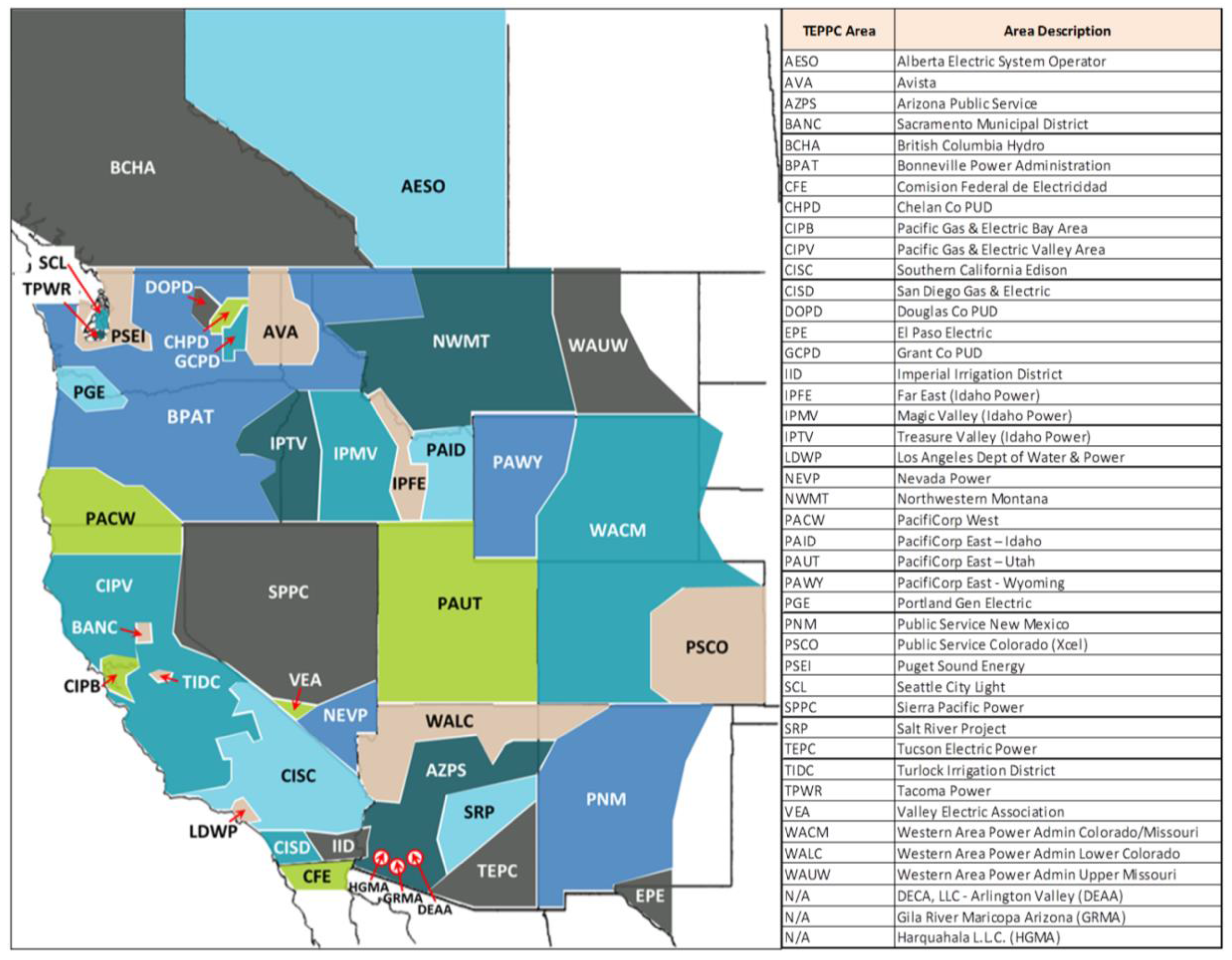
Since this study focuses on the desert southwest, specifically Arizona, the decision was to run balancing areas in Arizona nodally, and the rest of the Western Interconnect zonally. In order to do that, the transmission is aggregated into zones for all balancing areas, except for Arizona Public Service (AZPS), Salt River Project (SRP), Tucson Electric Power (TEPC), Western Area Power Administration Lower Colorado Region (WALC), Imperial Irrigation District (IID), and Public Service New Mexico (PNM), which are represented nodally. See Figure 2 [36] for a map of the Western Interconnect balancing areas. All simulation runs followed this naming convention.

Figure 2.
Western Electricity Coordinating Council (WECC) Balancing Areas Map [36].
A generation change to the TEPPC 2024 database was to close down all units at the Navajo Generating Station (NGS). The owners have announced that NGS will not be operating past December 2019, and so it was turned off for all of the runs in this study. It is a major change for generation in the Southwestern United States, due to its 2250 MW size.
It was mentioned previously that four hydropower scenarios are being considered in this study. These scenarios were selected then modeled in PLEXOS, and were based on the TEPPC 2024 Database. In each of the four hydropower scenarios, the hydropower generation (maximum capacity and monthly energy production) per month was determined through consultation with Reclamation, as will be described in the next section. For each Colorado River hydropower dam of interest, the monthly energy production was modified to a revised GWh/month using the information provided by Reclamation.
2.2. Water Data
An important part of this study was to identify plausible future water supply scenarios, and to understand how these might affect hydropower and operation of the bulk electrical system especially in the Southwestern United States. Reclamation uses the Colorado River Simulation System (CRSS) model as their primary long-term water-planning tool. CRSS is implemented as a computer program that simulates the operation of the major reservoirs on the Colorado River, providing information about the projected future state of the hydro system on a monthly basis, as described by the reservoir elevations, water releases from the dams, water flow throughout the system, water storage, and diversions to and return flows from water users. With the assistance of Reclamation, projected 2030 hydropower conditions were identified and converted into projected power and energy availability on a monthly basis for the Colorado River hydropower dams. These projections, in turn, were then translated into inputs for the production cost model PLEXOS, via its “Energy” mode for modeling hydropower using the “Economic Dispatch” option. Thus, within the constraints of monthly maximum power and allocation of energy production per month, as well as honoring ramp rate limitations and generator maximum/minimum limits due to either environmental flow limitations or generator capability, the hydropower was economically dispatched. The remaining hydropower in the WECC remained as projected and modeled in the TEPPC base case.
As part of its output, CRSS produces multiple scenarios of future hydrologic and operational conditions at many of the Colorado River Basin dams, including the nine hydropower dams of interest in this study. These scenarios, hereafter referred to as time series “traces” of future water conditions, represent monthly time series of possible future water conditions from 2012 through 2060, an example of which is shown in Figure 3. For the purpose of this project, the goal was to select future water scenarios for this study that are plausible and include drought conditions, and therefore, are within the red circles shown in Figure 3.
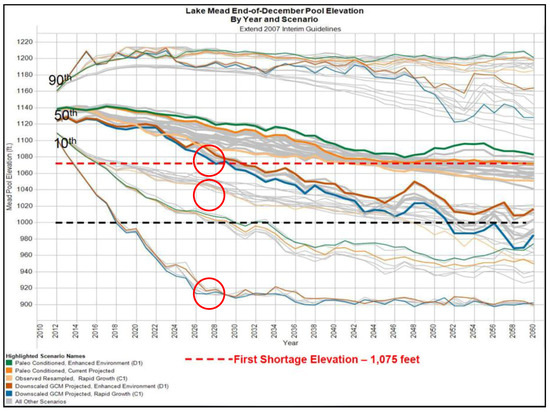
Figure 3.
Colorado River Simulation System (CRSS) projections of Lake Mead future pool elevations assuming various future water supply and demand scenarios [37].
For the purposes of this study, three future water scenarios have been recommended, to be drawn from the following four CRSS projections (the naming convention here mirrors that of the Colorado River Basin Water Supply and Demand Study [23]):
- Observed, resampled which bases a future projection upon historical river flows
- 50th percentile
- 10th percentile
- Downscaled GCM projected which projects future water supply based upon a general circulation model (GCM), and anticipates changes in the climate and therefore changes in water supply as compared to historical flows
- 50th percentile
- 10th percentile
In Figure 3 [37], three red circles are drawn on the vertical grid line corresponding to the year 2030, encapsulating these four projections. The uppermost of these three circles encloses traces for two of the scenarios: the Observed, resampled, 50th percentile, and the Downscaled GCM, 50th percentile. The Lake Mead pool elevation behind Hoover Dam for these scenarios ranges from normal operation (Mead elevation between 327 m (1075 ft) and 349 m (1145 ft) above sea level), and a Tier 1 shortage condition (Mead elevation between 320 m (1050 ft) and 327 m (1075 ft)). The shortage conditions are defined in the Interim Shortage Guidelines [20], and are summarized in Table 2 [38]. The middle circle in Figure 3 encompasses the Observed, resampled, 10th percentile case, and corresponds to a Tier 2 shortage condition (Mead elevation between 312 m (1025 ft) and 320 m (1050 ft)). The lowest of the three circles contains traces corresponding to the Downscaled GCM, 10th percentile, and indicate a Mead elevation between 274 and 280 m (900 and 920 ft). This level is below the low end of the third tier shortage condition shown in Table 2, and indicated by the black dashed line in Figure 3 at the 305 m (1000 ft) pool elevation. Looking forward in time from this circle shows that the Lake Mead elevation does not continue to decrease much through 2060, and thus it represents an appropriate “extreme drought” case. Due to the range of shortage operating conditions represented and the inclusion of an appropriate extreme drought case, projected hydro conditions from the year 2030 have been selected for use in the PLEXOS modeling.
Table 2.
Outline of the 2007 Interim Guidelines for water releases for Lake Mead [20].
With the assistance of Reclamation, projected 2030 hydropower conditions were converted into projected power and energy availability for the Colorado River hydropower dams. These projections, in turn, were then translated into PLEXOS inputs for its “Energy” mode for modeling hydropower using the “Economic Dispatch” options.
In order to select runs that made sense for this study, the simulations were ranked by inflow into Lake Powell as a proxy for overall water supply on the Colorado River Basin. The ranks of interest were those close to 10th and 50th percentile for the cases mentioned above. Focusing on those levels of inflows, the next step was to look at the elevation of Lake Mead and Lake Powell. Concerning power generation, it is important to note that while the water supply for any given year is important, the elevation of the reservoir is also pertinent. The reservoirs are set up for water storage to ensure consistent and reliable annual deliveries to downstream water users. Many years of low water supply in a row can cause the pool elevations to drop far enough that it can negatively affect power generation. Since extended drought may be a factor in the future, this study is examining that possibility, even though it has a very low probability of happening. As described above, these scenarios were selected from among the relevant CRSS simulations, and categorized as “historical hydro”, “moderate drought”, and “extreme drought”, and are shown in Table 3. Lake Powell and Lake Mead pool elevations are shown for the selected runs.
Table 3.
Lake Powell and Lake Mead pool elevations for the selected water scenarios.
To conclude, three water scenarios were identified from the CRSS model results, and were categorized as Historical Hydro, Moderate Drought, and Extreme Drought. According to the criteria set in the Interim Guidelines, water conditions were at “normal” levels for the Historical Hydro and TEPPC base case scenarios, under Tier 1 shortage conditions in the Moderate Drought case, and below Tier 3 shortage conditions in the Extreme Drought scenario. Indeed, in the Extreme Drought case, water levels behind Hoover and Glen Canyon dams were at the dead pool level, and therefore unable to generate power. This very low water scenario was derived from a CRSS model result (10th percentile, downscaled Global Climate Model), and thus is a plausible, albeit very low probability water future.
2.3. Renewable Additions
Solar is being added in the southwestern United States at a fast pace. Due to hydro’s unique ability to balance the electrical system load, including those effects due to variable renewable resources, this study investigated how system costs and the value of hydro change with additional renewable resources.
Solar data was generated using the System Advisor Model (SAM) [39]. SAM used the weather files from the NREL National Solar Radiation Database, and can output generation data for a particular site. Since weather and load are correlated, and the load in the TEPPC database is based on 2005 demand, solar data was based on 2005 solar. There is a correlation between the solar resource and load, since more sun and higher temperatures tend to increase air conditioning. The solar panels selected were single axis tracking, with a 33 degree tilt and 180 degree azimuth.
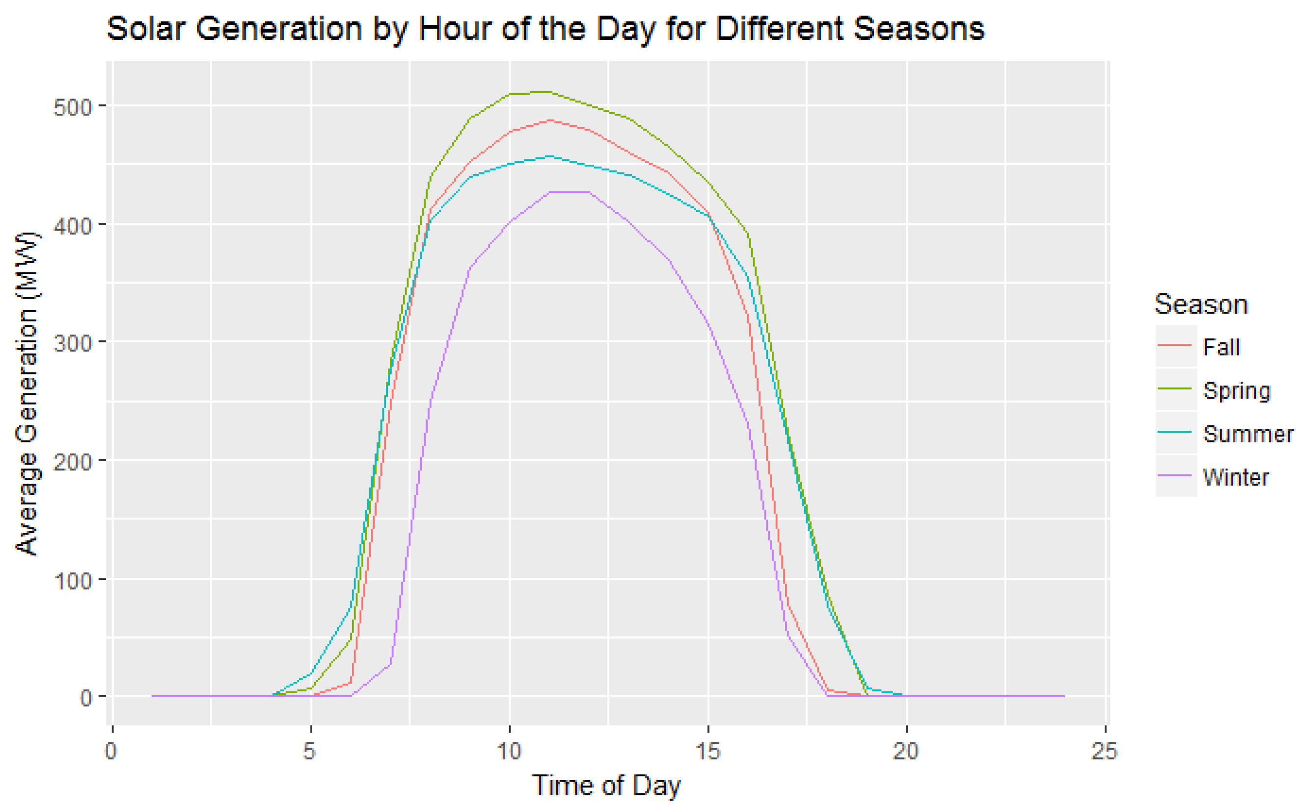
For the scenarios considered with additional solar power, 700 MW of solar was added in Arizona, 250 MW near Page, AZ, and 250 MW near Cameron, AZ, both in northern Arizona, 100 MW in Mesa, AZ, east of Phoenix and 100 MW in Tucson, AZ, in southern Arizona. The plant locations had similar power production patterns, most notably, high solar electricity output in the spring, specifically April, and a dip in electricity production in July and August (see Figure 4). In Arizona, spring tends to be very clear, while monsoon season, which peaks in July and August, brings rain and clouds over Arizona, especially in the afternoons. The solar electricity output reflects this weather pattern. Solar panels are also more efficient at cooler temperatures, which contributes to the higher photovoltaic (PV) generation in the spring season. This creates a mismatch between peak load hours, which are summer afternoons and evenings, and peak solar hours, which are midday hours in the spring.
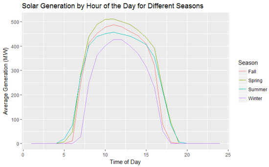
Figure 4.
The average hourly generation profiles for the four seasons for the proposed solar additions in Arizona.
2.4. Generation Scenarios
The generation scenarios were chosen to represent known and probable changes to the electricity grid in Arizona and the SW United States. Table 4 shows the matrix of 16 PLEXOS simulations that were conducted. In the table, the generation scenarios are the columns and the water scenarios are the rows. The next section will discuss the results obtained from these simulations.
Table 4.
Matrix of PLEXOS simulations. Hydro scenarios are listed in the first column, and generation scenarios in the first row.
3. Results
The PLEXOS results presented in this section were analyzed using R, an open source programming language for statistical computing and graphics. The R package, rplexos, was utilized first to converted PLEXOS output zip files to SQLite Databases, and also used to query the results. The first section of the results validates the PLEXOS model, and confirms that its scheduling and dispatching of generation to meet load was rational and consistent with actual system operation, by comparing reserve shortages, net imports, and dispatch stacks across scenarios. The subsequent sections focus on total generation cost, locational marginal prices (LMPs) in the WECC and in Arizona, hydro value, and value factor. The goals of the later sections are to better understand the value of hydropower on the electricity system.
3.1. Validation of Model
With production cost models like PLEXOS, it is important to make sure the perturbations, i.e., modifications to the base system model, do not cause unusual/unlikely behavior in simulating electrical system operation. In this section, different outputs were checked to validate that the model worked as expected, particularly that the unit commitment and economic dispatch were done in a way that makes sense.
In order to validate the model, a number of parameters were checked. First, it was confirmed that there was no unserved energy or dump energy. Unserved energy means that load could not be served by the available generation in the model. Given that the model has sufficient reserve margins, this would have indicated a problem. Dump energy occurs when the energy from “must run” units is larger than the load. With the current setup of the TEPPC 2024 database, this would also indicate a problem.
Reserve shortages show the amount, by GWh, that any region in the WECC is short on its reserve margin, usually set to 15% of expected load. Over the course of the 2024 model year, reserves provided in the model were about 61,325 GWh. A large amount of reserve shortages over the year would put the system at risk for not being able to recover from a contingency, such as a large generator shutting down unexpectedly. The sum of reserve shortages for all regions can be seen in Figure 5. Reserve shortages were less than 1 GWh over the year across the WECC with the exception of the Moderate Drought Solar scenario, which was 1.8 GWh. This is a very small percentage of the overall reserves provided.
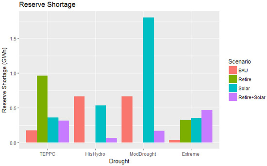
Figure 5.
Reserve shortages for the 16 test cases.
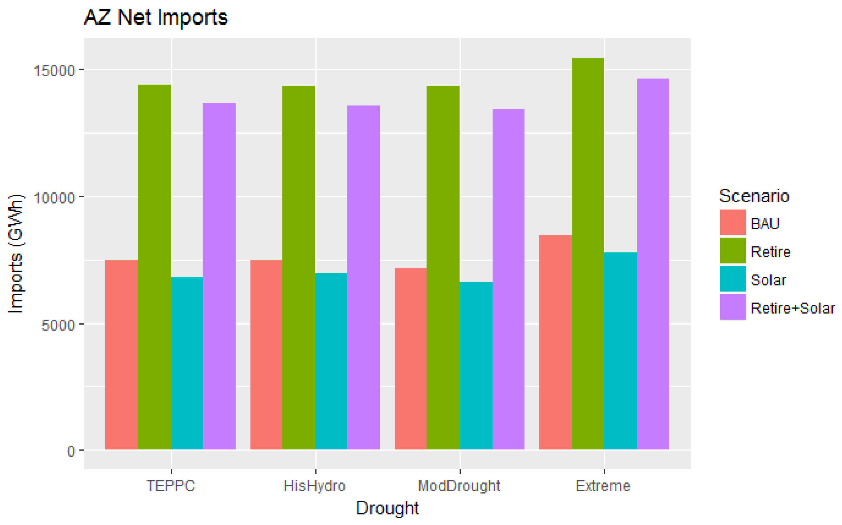
Figure 6 shows the net imports for Arizona. The retirement of Navajo Generating station increases net imports, which makes sense since it is the loss of a large coal generator in the state. The addition of solar reduces the net imports with Solar compared to BAU and Retire + Solar compared to Retire, which is also an expected result, since the solar increases the in-state electricity generation and so less imports would be needed. The net imports for Arizona are explainable and do not show unexpected changes.

Figure 6.
Net Imports for Arizona balancing areas compared across drought and generation scenarios.
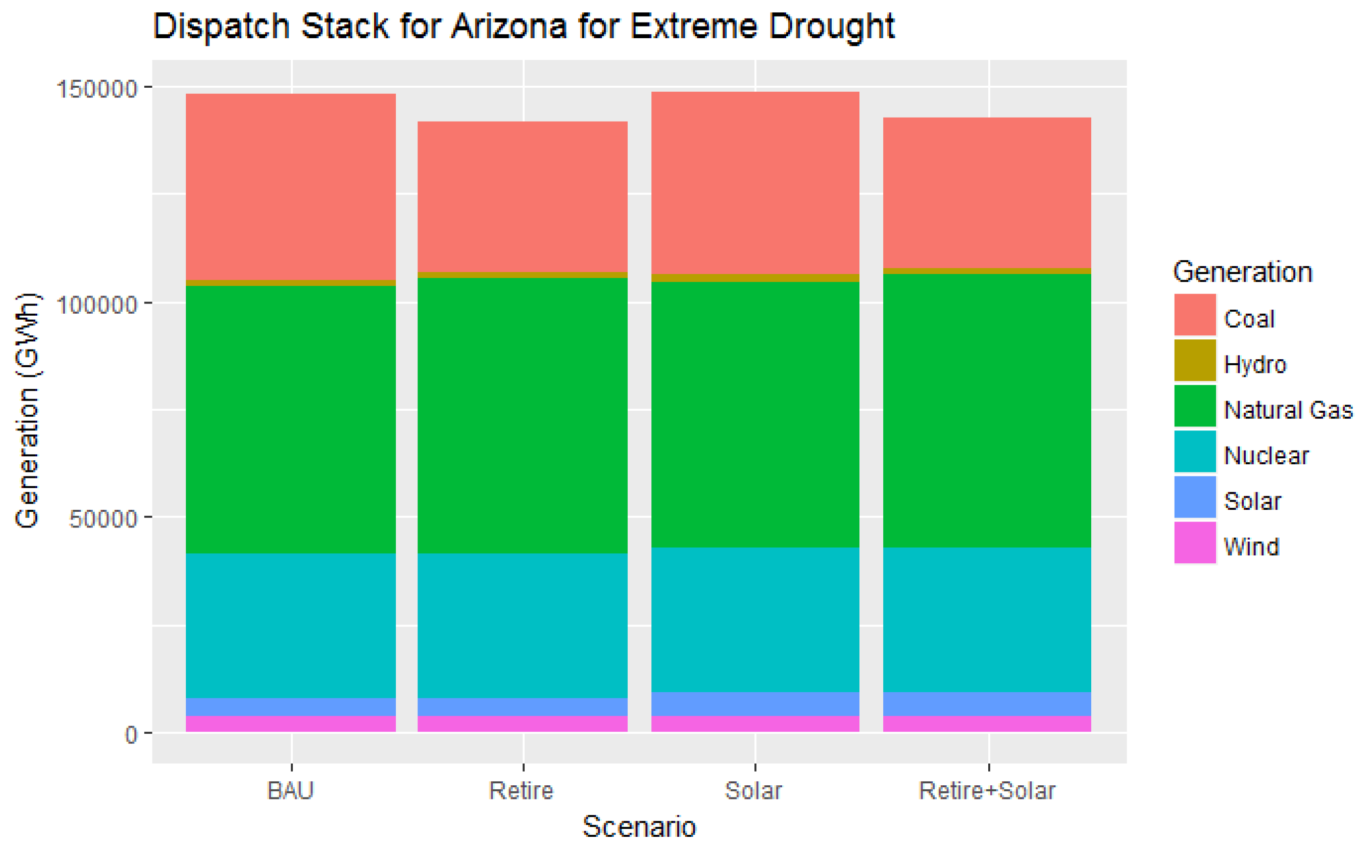
Figure 7 shows the dispatch stacks for the different generation scenarios for the Extreme drought water scenario for generation in Arizona. The stacks are changing in expected ways; there is less coal production in the scenarios with retirement and more solar production in the Solar Scenarios. The majority of the other generation is consistent between generation scenarios.

Figure 7.
The bar chart shows the generation stack for the year for the different generation stacks under the Extreme Drought water scenario for the state of Arizona.
The dispatch stack, reserve shortage, and net imports support the validation of this model. Given that these comparisons make sense with the specific perturbations made to the PLEXOS model, the model is behaving well, and the results are rational outcomes. The TEPPC base case was included in this section for reference. However, going forward, because the mode of dispatch in the test cases for the hydro is “economic” and not “fixed” (as it is in the TEPPC case), to preserve consistency in making comparisons between the hydro scenarios, the focus will be on results from the Historical Hydro, Moderate Drought, and Extreme Drought cases.
3.2. Generation Costs
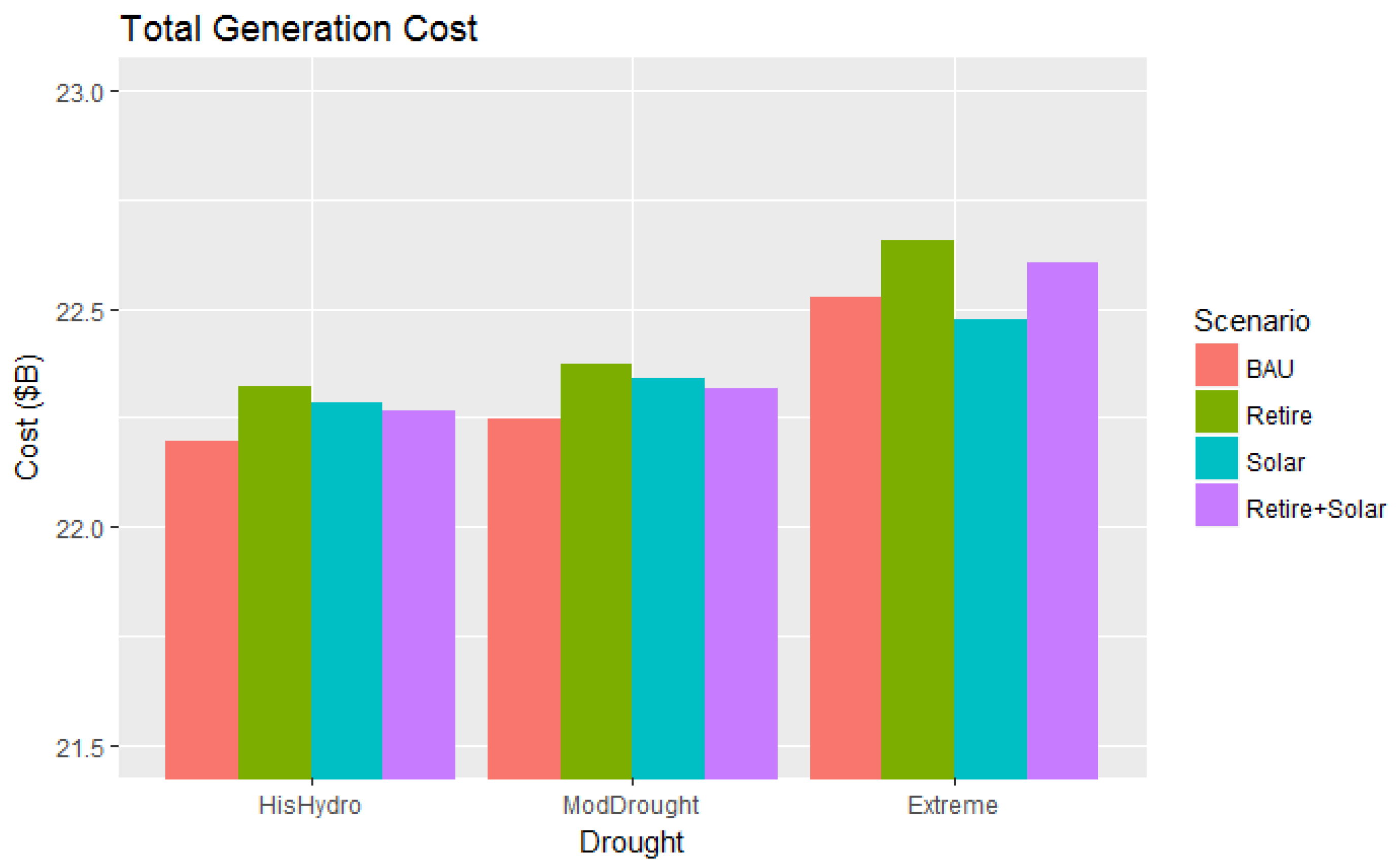
Total generation cost indicates the cost for generation to supply the load for the year 2024 given the generation, load, and drought scenario indicated. As Figure 8 shows, the Historical Hydro BAU has the lowest cost at $22.2B (billion), while Extreme Drought Retire has the highest at $22.66B. It is expected that the Extreme Drought Retire case would have the highest cost, since this case has the most constraints on generation with the retirement of coal and the low level of hydro generation. Given that reasoning, it would follow that the Historical Hydro Solar case should have the lowest cost. However, the Historical Hydro BAU case has the lowest cost, which tells us that the addition of solar does not always decrease the total system costs. In this case, the Historical Hydro Solar cases uses more high cost combustion turbine generation than the Historical Hydro BAU case. The Historical Hydro BAU case relies more on lower cost combined cycles, since there is more need for that generation throughout the day. All of the Extreme Drought generation scenarios have higher generation costs compared to the other two water scenarios. Focusing on a single generation scenario (e.g., compare the generation cost for the Retire scenario across the three water scenarios) it is evident that the trend is for the generation cost to increase as the magnitude of the drought increases. Comparing the Retire + Solar scenario with the Solar scenario, in the Historical Hydro and Moderate Drought scenarios, the generation costs are nearly the same (within <0.09%), but in the Extreme Drought scenario, the generation cost is more in the case with the retirement by 0.6% ($0.13B). In general, when comparing the Historical Hydro and Moderate Drought scenarios, the generation scenario has a larger impact on the cost than the water scenario. This is not true in the Extreme Drought scenario, where the effect of drought outweighs the generation changes. The numerical values mentioned above and plotted in Figure 8 are provided in Table A1 of Appendix A.
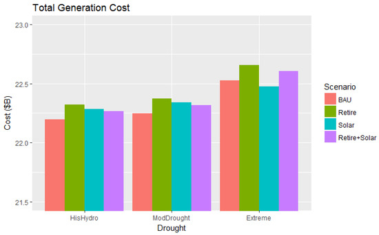
Figure 8.
The bar chart shows the total generation cost across the 12 scenarios. Note the graph starts at $21.5B.
3.3. Locational Marginal Pricing
Figure 9 compares the mean LMPs throughout the WECC for each scenario. The mean prices are all in the $36 range, with the highest mean LMPs seen with the Extreme Drought scenario. LMPs are used to price electricity in market systems, like California. In non-market balancing areas, like Arizona, LMPs give a sense of how expensive it is to provide electricity for that balancing area. LMPs will increase in some areas, and decrease in others when there is congestion on the transmission lines, ultimately leading to the purchase of higher-priced electricity in transmission constrained areas. As displayed in Figure 9, the WECC LMPs follow a pattern for the generation scenarios. Retire and Retire + Solar have higher LMPs, while the BAU and Solar scenarios have lower LMPs across the WECC. The highest overall average LMP is Extreme Drought Retire scenario, which makes sense, since it is scenario with the most constrained generation. The least expensive average LMP is seen with Historical Hydro Solar, which is the least constrained in terms of generation. When comparing similar generation scenarios within a hydro scenario (e.g., BAU with Solar, or Retire with Retire + Solar), the addition of solar always reduces the LMP.
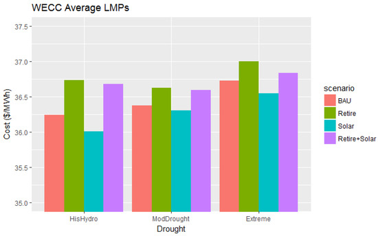
Figure 9.
This bar chart shows the WECC Average locational marginal prices (LMPs) for 2014 for the 12 scenarios. Note the bar chart starts at $35/MWh.
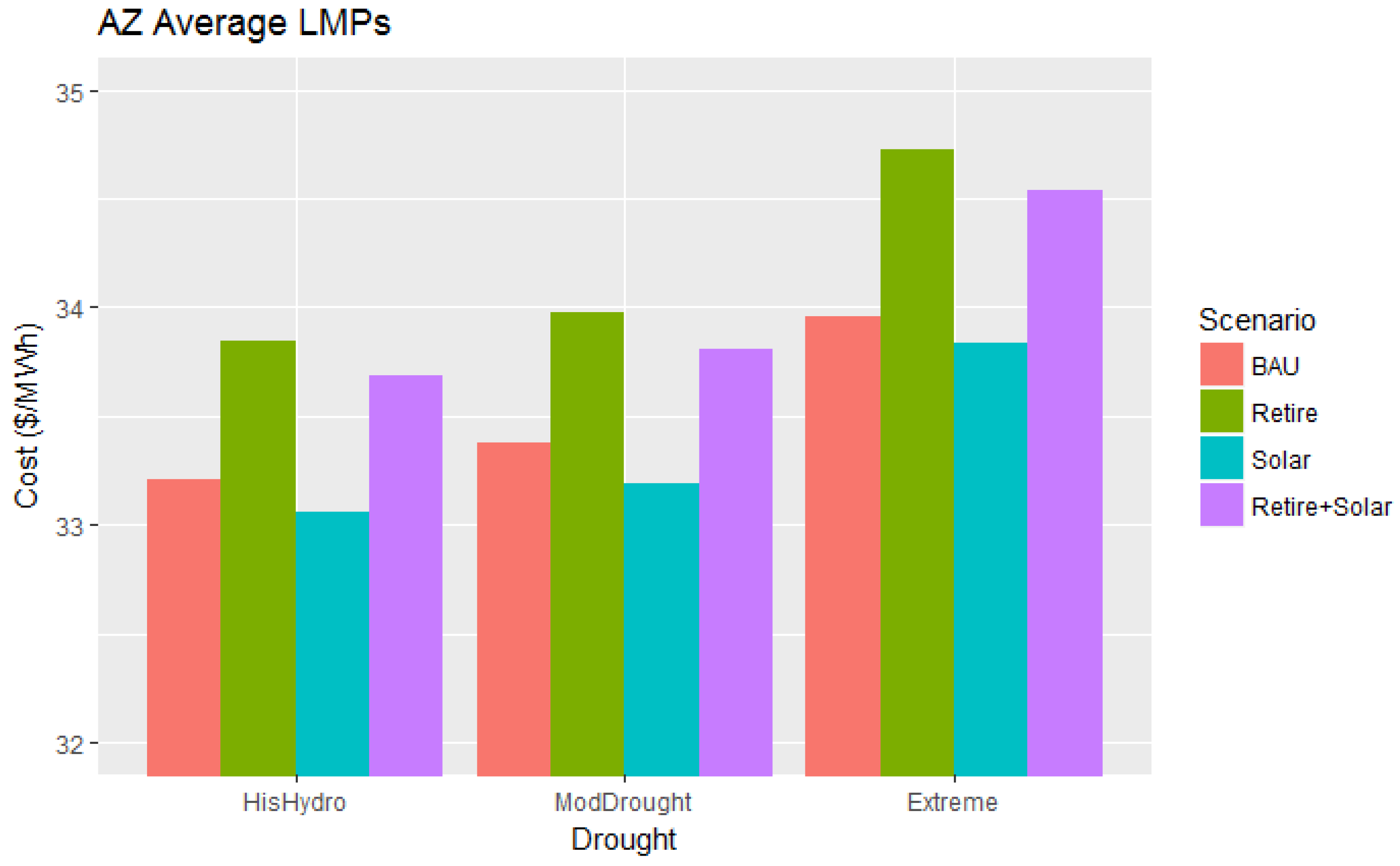
Figure 10 shows the mean LMPs experienced in Arizona balancing areas. The mean prices are all in the $33/MWh to $34/MWh range. A similar pattern for average LMPs is found in Arizona as for the WECC. The overall lowest LMP and highest LMP are the same as the WECC. Arizona, on the whole, has lower LMPs than the average WECC LMP, and the influence of retiring NGS is more pronounced (since NGS is in AZ). For numerical values associated with the bars plotted in Figure 9 and Figure 10, see Table A2 and Table A3 in Appendix A.

Figure 10.
This bar chart shows the LMPs in Arizona for the different scenarios. Note the bar chart starts at $32/MWh.
3.4. Value of Hydro Generation
Table 5 shows the amount of hydropower generation (GWh) for the Colorado River Basin, the generation from Hoover and Glen Canyon dams individually, and the shortage condition associated with the Interim Guidelines, as discussed earlier. This generation information was used to calculate a value of the hydropower as described below. The TEPPC base case is included in this table for reference.
Table 5.
Hydropower generation in the drought scenarios for the hydropower plants of interest along the Colorado River (see Table 1), for the power plants at Hoover and Glen Canyon dams, and the probable shortage condition, if applicable.
The goal of this work is to devise a rational method for determining the value of hydropower generation in electrical system balancing, and to apply the method to the generation and hydro scenarios considered in this study. Using the total generation cost and the amount of hydro generation, it is possible to calculate a value of the hydropower based upon the differences in generation between the scenarios. An estimated value for the difference in hydro generation between the drought scenarios is calculated by first determining the difference in total generation costs, between the cost in a given scenario and the cost in the Historical Hydro case, which had no drought:
Next, compute the difference in total hydropower generation, , between the amount in a given scenario and the amount in the Historical Hydro case:
The change in total production cost per MWh of hydropower, , can then be calculated as
A value for the difference in hydropower generation can then be determined by estimating the price paid to make up for the difference in hydropower. For the purpose of this work, a conservative estimate of the hydropower value, , was determined by taking the average LMP across the entire year for the WECC, , representing an average amount that would be paid for a MWh of energy, and adding to it the change in production cost per MWh of hydropower:
This value is interpreted as a conservative estimate of the price that would be paid for generation in lieu of the hydropower, since the average LMP across the WECC is less than the average LMP during the mainly high load and peak hours during which the Colorado River hydropower is used.
Table 6 shows this calculation for each of the hydro scenarios. For the Moderate and Extreme drought cases shown in Table 6, where 1342 and 8479 GWh less hydropower is generated, respectively, the additional cost per MWh of lost hydro was at $37.26/MWh and $38.92/MWh of hydro, respectively (see column 4). This implies the cost of energy to replace the hydro in these two cases was approximately $73.62/MWh and $75.64/MWh of missing hydropower, respectively. This number provides an indication of the value of the hydropower produced at these dams: the price to replace the missing hydro is roughly twice the price paid when the hydro is present. It is interesting to note that the value per MWh of the missing hydropower in the Extreme Drought scenario is slightly higher than that of the Moderate Drought scenario, indicating that as less hydro is available, higher cost generation is used as a replacement.
Table 6.
The difference in generation cost and hydro generation across the four drought scenarios along with an approximate value of the differences in hydro generation.
The process for determining the hydro value, HV, was repeated for each of the generation scenarios. The results of that process are summarized in Table 7, which compares the hydro value for the Moderate and Extreme Drought scenarios compared to the Historical Hydro. The hydropower in the Moderate Drought scenario has a consistent value across the generation scenarios, at about twice the value of the average LMP. The large amount of hydropower removed with the Extreme Drought case has a value around $75/MWh, except in the Solar scenario, which has a value of $57/MWh. The Historical Hydro Solar scenario required more higher-cost combustion turbine generation than the Extreme Drought Solar case, which resulted in a lower hydro value for the Extreme Drought Solar case.
Table 7.
The value of hydropower for the Moderate and Extreme Drought scenarios.
3.5. Value Factor
Adapting a technique used in a 2016 paper about the value of wind energy using a “value factor” [40], this study employed a concomitant method to confirm the value of hydro presented previously. The purpose of determining a value factor is to have a metric for comparing generation with a variable profile to that with a flat profile. The first step for calculating the value factor is to calculate the hydro-weighted average electricity price:
where t ∈ T denotes all hours of the year, Ht is the amount of hydro generation, and Pt is the hourly average LMP for WECC. The value factor is a ratio of the hydro-weighted average electricity price to the mean LMP for the year. (The mean LMPs for WECC are presented in Figure 9 and Table A2.)
Table 8 presents the value factors for the generation and drought scenarios. The value factor is highest for the Extreme Drought, and Retire and Retire + Solar scenarios at 1.11 and 1.10 for the other Extreme Drought scenarios. It is lowest at 1.06 for Historical Hydro BAU, Retire and Retire + Solar, and Moderate Drought Retire. As one would expect, with low cost hydro being used during high load, high LMP hours during the year, the value factor of hydro is always greater than one. As hydro generation decreases with increasing drought, its value factor increases; i.e., LMPs increase during peak hours, increasing the value of hydro generation during these hours. It is interesting that the value factor increases in the Solar case with Historical Hydro and Moderate Drought with respect to BAU, but stays the same in Extreme Drought. This is likely due to solar displacing hydro power during the day time hours and hydro production increasing in the non-solar houses, similar to what Chang [32] found. It is likely that there is not enough hydro in the extreme drought case to shift much in response to the additional solar.
Table 8.
This table presents the value factor for the hydro power in each scenario.
4. Discussion
This study used production cost modeling to examine the effects of specific future possibilities in the desert Southwest of the United States, taking into account generation scenarios and drought scenarios with the goal of better understanding how those possible future changes influence WECC and Arizona electrical system operating costs and the value of hydropower. PLEXOS was employed as the simulation tool with the TEPPC 2024 dataset used as the base model for WECC transmission and generation. Four generation scenarios were considered: the TEPPC base case, then TEPPC with coal retirement, added solar, or both. Three predicted future water scenarios were considered for Colorado River hydropower within the WECC, in addition to the TEPPC base case: Historical Hydro, which assumed availability of hydro similar to past years; Moderate Drought, with similar characteristics to past drought conditions; and Extreme Drought, which uses a forecasted future hydropower scenario occurring after several years of drought. All of these drought cases were derived from the U.S. Bureau of Reclamation’s CRSS model, and represent possible future water conditions (albeit of a low probability in the Extreme Drought case). To validate operation of the PLEXOS model, simulation outputs describing electrical system operation were analyzed, including the dispatch stack, reserve shortage, and net imports. These results support that the specific perturbations made to the PLEXOS model in implementing the generation and drought scenarios led to the conclusion that the model was behaving well, and producing results with rational outcomes.
Results from the simulations demonstrate that for generation costs and LMPs, constrained generation via retirement of the NGS coal plant and reduced hydro generation due to drought tended to lead to higher operating costs. In general, the Extreme Drought and Retirement cases had the highest costs. The addition of solar decreased LMPs for all scenarios, thought it did not reduce the system operating cost in all cases. This suggests that the addition of solar may result in some added costs, due to an increased use of higher-cost combustion turbines in addition to its associated system benefit of a low marginal cost.
The calculated value of the hydropower was about $73 to $75 per MWh for most scenarios, which would be the cost to replace the hydro generation. Thus, hydropower value is about twice the average price to provide electricity when compared to the average LMP. The calculated value factors also show that hydroelectric power is more valuable than the typical generator available during high load hours, since all of the value factors are greater than one. When comparing the value factor between different generation scenarios, it is evident that the value of hydro is higher when there is less hydro available, and when there is more solar generation.
While droughts cannot be controlled, generation to a certain extent can be. Building an electricity system that is resilient to drought may become more important in the future. Given the total generation cost and the average LMPs, it would seem that the Solar case has the most resiliency for the Extreme Drought, since costs and prices are the lowest for that water scenario. While predicting drought accurately is impossible, it is important to have margins to deal with drought if it happens. Moreover, hydropower was demonstrated here to be a particularly valuable generating resource in operating the electrical system, and its value generally increases with the addition of a variable generator such as solar, or with the loss of generation via drought.
Acknowledgments
The authors would like to thank David Hurlbut, Greg Brinkman and Scott Haase at the National Renewable Energy Laboratory for their input and insights, and to Energy Exemplar for providing an academic license to PLEXOS. Also, thank you to Rick Clayton at the U.S. Bureau of Reclamation for his assistance in creating the water scenarios. Lastly, thanks to Ignacio Losada Carreno and Roberto Puente Aranda, both NAU mechanical engineering undergraduates, for their help with data collection, analysis and visualization, and to Karin Wadsack, program director at NAU for her input and feedback.
Author Contributions
Dominique Bain was the primary author of this article, with guidance and contriburtions from her Ph.D. advisor, Dr. Tom Acker.
Conflicts of Interest
The authors declare no conflicts of interest.
Appendix A
Table A1.
Total Generation Cost ($B) for the 12 simulation scenarios.
Table A1.
Total Generation Cost ($B) for the 12 simulation scenarios.
| Drought Case- | BAU | Retire | Solar | Retire + Solar |
|---|---|---|---|---|
| Historical Hydro | 22.20 | 22.32 | 22.29 | 22.27 |
| Moderate Drought | 22.25 | 22.37 | 22.34 | 22.32 |
| Extreme Drought | 22.53 | 22.66 | 22.47 | 22.60 |
Table A2.
Average WECC LMP ($/MWh) for the 12 simulation scenarios.
Table A2.
Average WECC LMP ($/MWh) for the 12 simulation scenarios.
| -Drought Case | BAU | Retire | Solar | Retire + Solar |
|---|---|---|---|---|
| Historical Hydro | 36.24 | 36.73 | 36.01 | 36.68 |
| Moderate Drought | 36.37 | 36.62 | 36.30 | 36.59 |
| Extreme Drought | 36.73 | 37.00 | 36.54 | 36.84 |
Table A3.
Average AZ LMP ($/MWh) for the 12 simulation scenarios.
Table A3.
Average AZ LMP ($/MWh) for the 12 simulation scenarios.
| -Drought Case | BAU | Retire | Solar | Retire + Solar |
|---|---|---|---|---|
| Historical Hydro | 33.21 | 33.84 | 33.06 | 33.68 |
| Moderate Drought | 33.38 | 33.97 | 33.19 | 33.81 |
| Extreme Drought | 33.95 | 34.73 | 33.83 | 34.53 |
References
- U.S. Department of Energy. Staff Report to the Secretary on Electricity Markets and Reliability; U.S. Department of Energy: Washington, DC, USA, 2017.
- Wiser, R.; Bolinger, M.; Barbose, G.; Darghouth, N.; Hoen, B.; Mills, A.; Rand, J.; Millstien, D.; Porter, K.; Widiss, R.; et al. 2016 Wind Technologies Market Report; Wind Technologies: Berkeley, CA, USA, 2017. [Google Scholar]
- Bolinger, M. Utility-Scale Solar 2016: An Empirical Analysis of Project Cost, Performance, and Pricing Trends in the United States; Electricity Markets and Policy Group: Berkeley, CA, USA, 2017.
- Lazard. Lazard’s Levelized Cost of Energy Analysis—version 11.0; New York, NY, USA, 2017. [Google Scholar]
- Gleick, P.H. Impacts of California’s Ongoing Drought: Hydroelectricity Generation; Pacific Institute: Oakland, CA, USA, 2016. [Google Scholar]
- Barbose, G. U.S. Renewables Portfolio Standards 2017 Annual Status Report; Electricity Markets and Policy Group: Berkeley, CA, USA, 2017.
- Brady, D.; Mufson, S. The West’s Largest Coal-Fired Power Plant is Closing. Not Even Trump Can Save It. Available online: https://www.washingtonpost.com/news/energy-environment/wp/2017/02/14/the-wests-largest-coal-fired-power-plant-is-closing-not-even-trump-can-save-it/?utm_term=.845c35778041 (accessed on 24 October 2017).
- Public Service Company of New Mexico. PNM 2017-2036 Integrated Resource Plan; Public Service Company of New Mexico: Albuquerque, NM, USA, 2017. [Google Scholar]
- Hurlbut, D.; Haase, S.; Barrows, C.; Bird, L.; Brinkman, G.; Cook, J.; Day, M.; Diakov, V.; Hale, E.; Keyser, D.; et al. Navajo Generating Station & Federal Resource Planning; National Renewable Energy Laboratory (NREL): Golden, CO, USA, 2016; Volume 1.
- California ISO. What the Duck Curve Tells Us about Managing a Green Grid. Available online: https://www.caiso.com/Documents/FlexibleResourcesHelpRenewables_FastFacts.pdf (accessed on 12 November 2017).
- GE Energy. Western Wind and Solar Integration Study; National Renewable Energy Laboratory (NREL): Golden, CO, USA, 2010.
- Lew, D.; Brinkman, G.; Ibanez, E.; Hodge, B.; King, J. The Western Wind and Solar Integration Study Phase 2; National Renewable Energy Laboratory (NREL): Golden, CO, USA, 2012.
- U.S. Department of Energy. 20% Wind Energy By 2030: Increasing Wind Energy’s Contribution to U.S. Electricity Supply; U.S. Department of Energy: Washington DC, USA, 2008.
- Porter, K.; Fink, S.; Rogers, J.; Mudd, C.; Buckley, M.; Clark, C.; Hinkle, G. PJM Renewable Integration Study: Review of Industry Practice and Experience in the Integration of Wind and Solar Generation; Exeter Associates, Inc.: Columbia, MD, USA; GE Energy: Schenectady, NY, USA, 2012. [Google Scholar]
- Venkataraman, S.; Jordan, G.; Piwko, R.; Freeman, L.; Helman, U.; Loutan, C.; Rosenblum, G.; Xie, J.; Zhou, H.; Kuo, M. Integration of Renewable Resources: Operational Requirements and Generation Fleet Capability at 20% RPS; California ISO: Folsom, CA, USA, 2010. [Google Scholar]
- Acker, T.L.; Zavadil, R.; Potter, C.; Flood, R. Wind integration cost impact study for the Arizona public service company: Modeling approach and results. Wind Eng. 2008, 32, 339–354. [Google Scholar] [CrossRef]
- Acker, T. IEA Wind Task 24: Integration of Wind and Hydropower Systems; International Energy Agency: Paris, France, 2011. [Google Scholar]
- Acker, T.; Pete, C. Western Wind and Solar Integration Study: Hydropower Analysis; National Renewable Energy Laboratory (NREL): Golden, CO, USA, 2012.
- Zavadil, R. Avista Corporation Wind Integration Study; Avista Corporation: Knoxville, TN, USA, 2007. [Google Scholar]
- Bureau of Reclamation. Interim Shortage Guidelines; Bureau of Reclamation: Washington, DC, USA, 2007.
- Bureau of Reclamation. Bureau of Reclamation Hydroelectric Powerplants; Bureau of Reclamation: Washington, DC, USA, 2014.
- Bureau of Reclamation. Bureau of Reclamation—Dams. Available online: http://www.usbr.gov/projects/dams.jsp#Initial_P (accessed on 5 November 2015).
- Bureau of Reclamation. Colorado River Basin Water Supply and Demand Study; Bureau of Reclamation: Washington, DC, USA, 2012.
- Bureau of Reclamation; National Park Service. Appendix K: Hydropower Systems Technical Information and Analysis; National Park Service: Salt Lake City, UT, USA, 2016.
- Bureau of Reclamation. Technical Report B-Supply; Bureau of Reclamation: Washington, DC, USA, 2012.
- U.S. Department of the Interior; Bureau of Reclamation. Annual Operating Plan for Colorado River Reservoirs 2015; U.S. Department of the Interior: Washington, DC, USA, 2014.
- U.S. Energy Information Administration Utility Scale Facility Net Generation from Hydroelectric (Conventional) Power. Available online: https://www.eia.gov/electricity/annual/html/epa_03_14.html (accessed on 12 November 2017).
- U.S. Energy Information Administration Oregon State Profile and Energy Estimates. Available online: https://www.eia.gov/state/analysis.php?sid=OR (accessed on 12 November 2017).
- U.S. Energy Information Administration Washington State Profile and Energy Estimates. Available online: https://www.eia.gov/state/analysis.php?sid=WA (accessed on 12 November 2017).
- Madani, K.; Lund, J.R. Estimated impacts of climate warming on California’s high-elevation hydropower. Clim. Chang. 2010, 102, 521–538. [Google Scholar] [CrossRef]
- Tarroja, B.; AghaKouchak, A.; Samuelsen, S. Quantifying climate change impacts on hydropower generation and implications on electric grid greenhouse gas emissions and operation. Energy 2016, 111, 295–305. [Google Scholar] [CrossRef]
- Chang, M.K.; Eichman, J.D.; Mueller, F.; Samuelsen, S. Buffering intermittent renewable power with hydroelectric generation: A case study in California. Appl. Energy 2013, 112, 1–11. [Google Scholar] [CrossRef]
- Boehlert, B.; Strzepek, K.M.; Gebretsadik, Y.; Swanson, R.; McCluskey, A.; Neumann, J.E.; McFarland, J.; Martinich, J. Climate change impacts and greenhouse gas mitigation effects on U.S. hydropower generation. Appl. Energy 2016, 183, 1511–1519. [Google Scholar] [CrossRef]
- Ibanez, E.; Magee, T.; Clement, M.; Brinkman, G.; Milligan, M.; Zagona, E. Enhancing hydropower modeling in variable generation integration studies. Energy 2014, 74, 518–528. [Google Scholar] [CrossRef]
- Transmission Expansion Planning and Policy Committee. TEPPC 2014 StudyProgram; Transmission Expansion Planning and Policy Committee: Salt Lake City, UT, USA, 2014. [Google Scholar]
- Western Electricity Coordinating Council (WECC). TEPPC Study Report 2024 PC1 Common Case; Western Electricity Coordinating Council: Salt Lake City, UT, USA, 2015. [Google Scholar]
- Gross, D. Colorado River Simulation System (CRSS), Overview and Use in Planning and Operation in the Colorado River Basin; Arizona Department of Water Resources: Phoenix, AZ, USA, 2015.
- Mahmoud, M. Colorado River Planning and Modeling. Available online: https://s3-us-west-2.amazonaws.com/gios-web-img-docs/docs/dcdc/website/documents/ASU_Presentation_MohammedMahmoud.pdf (accessed on 12 November 2017).
- National Renewable Energy Laboratory System Advisor Model (SAM). Available online: https://sam.nrel.gov/ (accessed on 27 July 2016).
- Hirth, L. The benefits of flexibility: The value of wind energy with hydropower. Appl. Energy 2016, 181, 210–223. [Google Scholar] [CrossRef]


© 2018 by the authors. Licensee MDPI, Basel, Switzerland. This article is an open access article distributed under the terms and conditions of the Creative Commons Attribution (CC BY) license (http://creativecommons.org/licenses/by/4.0/).