Article

Co-Planning of Demand Response and Distributed Generators in an Active Distribution Network

1
School of Electrical Engineering, Wuhan University, Wuhan 430072, China
2
Department of Electrical Engineering, The Hong Kong Polytechnic University, Hong Kong, China
3
Department of Electrical Power Engineering, Shanghai University of Electric Power, Shanghai 200090, China
*
Author to whom correspondence should be addressed.
Energies 2018, 11(2), 354; https://doi.org/10.3390/en11020354
Submission received: 9 January 2018 / Revised: 22 January 2018 / Accepted: 23 January 2018 / Published: 2 February 2018
(This article belongs to the Special Issue Solar Energy Harvesting, Storage and Utilization)

Abstract

:
The integration of renewables is fast-growing, in light of smart grid technology development. As a result, the uncertain nature of renewables and load demand poses significant technical challenges to distribution network (DN) daily operation. To alleviate such issues, price-sensitive demand response and distributed generators can be coordinated to accommodate the renewable energy. However, the investment cost for demand response facilities, i.e., load control switch and advanced metering infrastructure, cannot be ignored, especially when the responsive demand is large. In this paper, an optimal coordinated investment for distributed generator and demand response facilities is proposed, based on a linearized, price-elastic demand response model. To hedge against the uncertainties of renewables and load demand, a two-stage robust investment scheme is proposed, where the investment decisions are optimized in the first stage, and the demand response participation with the coordination of distributed generators is adjusted in the second stage. Simulations on the modified IEEE 33-node and 123-node DN demonstrate the effectiveness of the proposed model.

1. Introduction

Recently, the penetration of renewables increases constantly in the modern distribution network (DN), due to their worldwide availability and sustainability [1,2,3]. In addition to the benefits of conventional distributed generations, such as energy loss reduction and infrastructure upgrade deferment [4], renewable energy sources also play significant roles in carbon emission reduction, energy conservation, and the promotion of fossil fuel alternatives. Nevertheless, due to their intermittent and variable nature, renewables, such as wind power and solar energy, are known as non-dispatchable and uncontrollable sources. The expanding integration of renewables will introduce tremendous difficulties in order to maintain power system reliability [5,6,7]. The bidirectional power flow that emerges with renewables installation leads to either a rise or a drop in voltage, depending on the output fluctuation of renewables. In addition, a large injection of renewables may lead to substations being adversely overloaded and line congestion.
In order to ease these negative impacts, dispatchable distributed generator (DG) is usually considered as an energy supplement and reserve, by reason of its controllability and small ramping limit [4]. Demand response (DR) has been commonly known as an efficient approach in peak load reduction [8]. Generally, the DR program is designed to adjust terminal customers’ electricity consumption by offering financial incentives, or providing time-varying prices, in order to decrease electricity demand when the system operates at high-risk conditions [9,10]. By the reason of its successful application in load profile reconstruction, DR also provides a promising alternative in helping renewable energy accommodation [6,11,12,13,14]. The authors of [6] propose an coordinated operation strategy of reserve and DR to cope with the uncertainty of renewable energy resources. Bitaraf and Rahman [11] focus on wind power curtailment reduction via coordinated scheduling of DR and energy storage. Zhao et al. [13] propose a multi-stage, unit commitment decision model in a transmission network, wherein the DR program is considered as a reserve source to accommodate integrated wind farms. A multi-period optimal power flow (OPF )problem, with flexible aggregated demand response and renewable generation, is solved in [12]. In [14], a day-ahead DR scheduling decision, as well as real-time micro-turbine and renewables operation strategy for a micro-grid is proposed. However, from the perspective of DN operation and planning, the DG and DR should be coordinated to efficiently fulfill the energy management problem. When the actual renewable energy is significantly redundant or deficient, the system operation constraints are not guaranteed. Furthermore, the price-sensitive load itself has uncertainties as well, and will considerably affect the optimization results. Hence, the coordinated operation of DG and DR is necessary to achieve the overall economic cost, system reliability, and environmentally benefits.
In the existing literature, DR is usually assumed to be a basic feature of a particular part of demand [9,10,12,13,14,15]. However, to enable and support this feature, the demand should be installed with specific equipment, such as a load control switch (LCS), and the conventional meters should be upgraded to advanced metering infrastructure (AMI). Only with these demand response facilities (DRFs) installed at the demand side can customer energy usage be measured and remotely controlled, as well responding to real-time system operation requests [16,17,18]. As a result, many household and commercial appliances, such as air conditioners, electric water heaters, and pool pumps, can participate in the DR program [19]. Some reports and papers [16,20,21] have conducted cost-benefit analyses of installing this equipment and DR program adoption. For example, report [16] gives a general introduction to different types of DR, and the benefit or cost to install each kind of DR is analyzed in U.S. In [20,21], a discussion about the capital return of the investment for DRFs in Europe is presented, in which the financial reliability and social welfare benefits of DR are considered. The conclusions in [16,21] indicate that the investment and operation cost for DR program should contain not only procurement and installation costs of LCS and AMI, but also incentive payments and education fees to customers. In particular, the investment cost for DG and DRFs will increase when the renewables penetration becomes larger. Although these works demonstrate the importance and necessity of optimizing DRF installation, they only give out a general discussion from economic aspects. To the best knowledge of the authors, the DRF planning methodology in a distribution system is not yet proposed. The DRF installation methodology that is able to accommodate the uncertainty of renewable energies is in especially urgent demand. Hence, in this paper, an optimization model for coordinated investment of DG and DRF, considering both demand and renewable uncertainty, is proposed, to address aforementioned operational issues.
In this paper, we propose a two-stage, robust optimization-based model for coordinated investment of DG and DRF, aiming at accommodating the uncertainties of renewables and load demand. The investment framework is presented in Figure 1. The investment of DG and DRF are optimized for cost minimization, so that the outputs of DG and DR can be coordinated and adjusted for distribution network operation. Robust optimization is adopted to ensure the robustness to uncertainties, by satisfying the DN operation limitation in a worst-case scenario. Wherein, the stepwise linearization approximation (SLA) method is adopted in the modified price-elastic demand response model, to describe the DR participation in DN operation. Finally, the column-and-constraint generation algorithm (CCG), combined with the outer approximation (OA) linearization method, are implemented to solve this optimization problem.
The rest of this paper is organized as follows. The demand response model is described in Section 2. Section 3 presents the mathematic formulation and the dual problem, and the solution methodology is presented in Section 4. Case studies to verify the proposed model are analyzed and discussed in Section 5. The conclusions are given in Section 6.

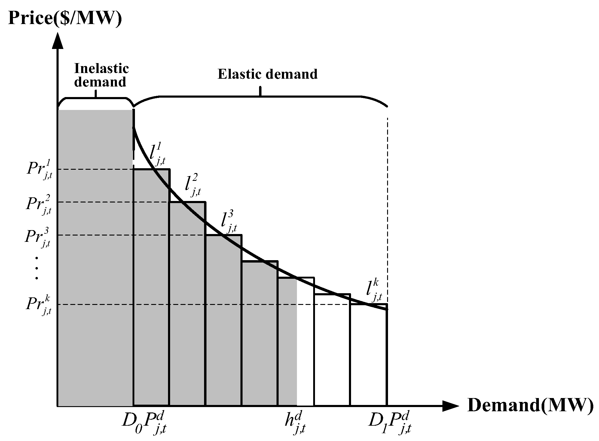
2. Demand Response Model

In the proposed demand response model, we assume the load at each DR bus is divided into inelastic and elastic parts. Considering the basic inelastic electricity consumption, only the part of demand that is flexible in electricity usage is selected as the DR program by investing DRFs. Other electricity demand, such as in schools and hospitals, is not affected by electricity price. A linearized price-elastic demand response (PEDR) model is implemented in the second stage to adjust the first-stage investment decisions. The power demand is usually modeled using a price-elastic curve [13,14,22], the expression of which is given as below:
P j , t d = A ( P r j , t ) γ
where P j , t d and Prj,t denote power demand and electricity price, respectively, A is the proportion and index constant parameters given in [22], and γ is the price elasticity which describes the sensitivity of load demand as to the change of price. For a given A and γ, the DN revenue from electricity consumption is equal to the integral of the constant inelastic demand and the price-elastic curve (present as r j , t d ), as shown in Figure 2.
Unfortunately, (1a) is non-convex. Thus, to remove nonlinear terms, the stepwise linearization approximation (SLA) is adopted to estimate the grid revenue contributed by DR program, which is modelled with the following auxiliary variables and constraints:
r j , t d = k K P r j , t k d j , t k
0 < d j , t k < l j , t k , j J , t T , k K
where d j , t k is the auxiliary variable recommended for demand at step k, l j , t k is the kth step length of the stepwise function, and P r j , t k is the corresponding electricity price. It is noted that P r j , t k stringently decreases with k, so that the DR program constraints are given as
h j , t d = D 0 P j , t d + k K d j , t k , j J , t T
D 0 P j , t d h j , t d D 1 P j , t d , j J , t T , k K
where h j , t d in (3a) donates the actual demand at DR node which is composed of constant inelastic demand and elastic demand. Constraint (3b) gives the upper and lower bound of the elastic demand.

3. Mathematical Formulation

3.1. Objective Function

The investment objective is to minimize the total cost, so as to find out the optimal allocation location of the DRF and DG. The objective function is to optimize the total costs and revenues during the whole planning horizon, which is formulated as:
min C i n v + C o p e + C a d n C e a r n + C p e n a
Overall, the function includes five parts, which are investment costs (Cinv), operation and maintenance costs for DGs (Cope), energy transaction cost (Cadn), DN revenue (Cearn), and penalty costs for operation violation (Cpena).
C i n v = C i n v d r + C i n v d g
C i n v d r = ε j J ( α j d r β j d r p j , p e a k d , e x p C C l c s + α j d r C C a m i )   + ϕ j J α j d r ( C C e d u + C C i n c )
C i n v d g = ε j J b B α j d g β j , b d g τ d g C C d g
Herein, the total investment cost is defined in (4b), which consists of the costs of DRFs and DGs, respectively. The investment cost of the DRF defined in (4c) contains two terms. The first term is the procurement and installation cost of LCS and AMI. The second term contains the education cost and financial incentive cost paid to electricity users for DR promotion. The investment cost of DG is defined in (4d). Notice that only the procurement and installation cost of LCS and DG has a linear relationship with their capacity. The capital recovery factor ε in (4c) and (4d) is utilized to transform the total investment cost into daily cost [23].
C o p e = C o m + C f u
C o m = t T ( j J C C o m d g P j , t d g + n N w t C C o m w t P n , t w t + n N P V C C o m p v P n , t p v )
C f u = t T j J C C f u d g P j , t d g
Equations (4e)–(4l) give the detailed expression of the operation costs and revenues, which contain the operation and maintenance cost of the DG, wind turbine (WT), and photovoltaic generator(PV), respectively; the fuel cost of DG; the energy transaction cost with the main-grid; and the revenue by selling electricity to customers. The operation and maintenance cost for WT and PV in (4f) are normally considered as the regular refurbishment and maintenance cost arisen from the depreciation with daily operation [24]. Additionally, the fuel cost of DG is dependent on the total energy generation, as illustrated with equation (4g).
C a d n = t T ( P r i n P i n , t P r o u t P o u t , t )
C e a r n = C d r + C c o n + C u n c
C d r = t T j J r j , t d
C c o n = t T j J ( 1 ( 1 D 0 ) η j ) P j , t d , e x p P r t
C u n c = t T j J ( 1 ( 1 D 0 ) η j ) P j , t d , e x p R j , t d P r t
The electricity exchange between DN and the main grid is presented as (4h). Considering the uncertain load demand, the DN revenue in (4i) is divided into three parts: the revenue from DR-enabled demand in (4j), the expected revenue from DR-not-enabled demand in (4k), and the uncertain revenue that is violated from its expected value in (4l).
C p e n a = C p e n a v o l + C p e n a l i n e + C p e n a s u b
C p e n a v o l = t T j J C C p e n a ( S j , t l v + S j , t u v )
C p e n a l i n e = t T i Ω j C C p e n a ( S i , t l c a p + S i , t u c a p )
C p e n a s u b = t T C C p e n a ( S t l s u b + S t u s u b )
In Equations (4m)–(4p), the penalty costs are expressed as constraint violations of voltage fluctuation, line congestion, and substation overload, which are computed by multiplying slackness variables with their penalty fees.

3.2. Constraint

The economic and technical constraints describing the investment and daily operation are listed in this subsection:
(1) The physical and technical constraints that describe the limitation of investment decision. The limitation of maximum number of DRF and DG investment locations is given in (5a) and (5b). The limitations of DG and DR capacities under a DN node are given in (5c) and (5d). In order to reduce the non-linearity and computing burden of the problem, the bilinear terms α j d r β j d r and α j d g β j , b d g are replaced by the auxiliary variables η j , t d r and γj,b, which are defined and limited by constraints (5e)–(5h). In addition, the capital recovery factor is defined in (5j).
j J α j d r N j
j J α j d g N j
0 β j , b d g B j m a x , j , b
0 β j d r 1 , j
η j d r = α j d r β j d r , j
0 η j d r α j d r , j
γ j , b = α j d g β j , b d g , j , b
0 γ j , b α j d g B m a x , j , b
α j d r , α j d g { 0 , 1 } , γ j , b , β j , b d g Z + , j , b
ε = ϕ z ( 1 + z ) l ( 1 + z ) l 1
(2) The physical and technical constraints describing the DR-enabled DN operation. The branch flow model (BFM) proposed in [25,26] is further simplified for distribution network modeling [27], which is described with constraints (6a)–(6c). Equation (6d) fixes the voltage at the substation as V0. Constraints (6e)–(6j) are the linearized PEDR model, in which the uncertainty of the load demand is considered by introducing the deviation rate R j , t d from expected value. Constraints (6k) and (6l) guarantee the energy consumption with DR investment is no smaller than original consumption, and the electricity bill for consumers with DR investment is no larger than the original bill. The constraints (6m)–(6n) express the energy exchange between DN and main grid, where Pin represent power purchase from the main grid, and Pout means DN sells energy to the main grid. Constraint (6o) gives the substation capacity limitation. The output limitation of DG and local reactive compensation devices are presented in constraints (6p)–(6q). Constraint (6r) is to guarantee that the power supply can satisfy the total demand with reserve factor θ. Constraint (6s) gives the voltage fluctuation limitations, and constraint (6t) guarantees the active power flow within the line capacity. It is worth noting that the operation constraints in (6o), (6s)–(6t) are relaxed, with positive variables S j , t u v , S j , t l v , S t u s u b , S t l s u b , S i i , t u c a p , and S i i , t l c a p , so that the penalty cost for operation violation can be computed.
P j , t = i Ω j P i , t + h j , t d n N w t P n , t w t n N p v P n , t p v j J P j , t d g , j , t
Q j , t = i Ω j Q i , t + Q j , t d s v N s v Q s v , t s v c , j , t
V j , t = V i , t + r i j P i , t + x i j Q i , t V 0 , i Ω j , j , t
V j , t = V 0 , j = 1 , t T
r j , t d = k K P r j , t k d j , t k , k , j
h j , t d = D 0 P j , t d , e x p ( 1 + R j , t d ) + k K d j , t k , k , j , t
D 0 P j , t d , e x p ( 1 + R j , t d ) h j , t d D 1 P j , t d , e x p ( 1 + R j , t d ) , j , t
0 < d j , t k < l j , t k , k , j , t
Q j , t d = Q j , t d , e x p ( 1 + R j , t d ) , j , t
μ l o w , j , t d 1 + R j , t d μ u p , j , t d , j , t
k K d j , t k t T j J ( 1 D 0 ) η j P j , t d , e x p ( 1 + R j , t d ) , j , t
t T j J r j , t d t T j J ( 1 D 0 ) η j P j , t d , e x p ( 1 + R j , t d ) P r t , j , t
P j , t = P i n , t P o u t , t , j = 1 , t
P i n , t 0 , P o u t , t 0 , t
P m i n s u b S t l s u b P j , t P m a x s u b + S t u s u b , j = 1 , t
0 P j , t d g γ j , b τ d g , j , t
0 Q s v , t s v c Q m a x , s v , t s v c s v , t
t T ( j J b B γ j , b τ m t + n N w t P u p , n , t w t + n N p v P u p , n , t p v ) θ t T j J P j , t d , e x p
1 σ S j , t l v V j , t 1 + σ + S j , t u v , j , t
P i j c a p S i j , t l s u b P i , t P i j c a p + S i j , t u s u b , i Ω j , j , t
S j , t u v , S j , t l v , S t u s u b , S t u s u b , S i , t u c a p , S i , t l c a p 0 , i Ω j , j , t

3.3. Uncertainty Set

In this paper, three polyhedral uncertainty sets are defined for the wind power, solar energy, and the load demand, respectively, given as follows,
U w t = { P n , t w t :
Γ l o w w t t T w W P n , t w t t T w W P m e a n , n , t w t Γ u p w t ,
μ u p , n , t w t P m e a n , n , t w t P n , t w t μ l o w , n , t w t P m e a n , n , t w t , n N w t , t }
U p v = { P n , t p v :
Γ l o w p v t T n N P V P n , t p v t T n N P V P m e a n , n , t p v Γ u p p v ,
μ u p , n , t p v P m e a n , n , t p v P n , t p v μ l o w , n , t p v P m e a n , n , t p v , n N p v , t }
U d = { h j , t d :
Γ l o w d 1 + t T j J R j , t d n t n j Γ u p d ,
μ l o w , j , t d 1 + R j , t d μ u p , j , t d , j , t }
In (7a) and (7b), we assume that the wind power and solar energy outputs are within an interval where P m e a n , n , t w t , p v represents the mean value of their outputs. This interval can generated through μ l o w , n , t w t , p v / μ u p , n , t w t , p v . The actual hourly output P n , t w t , p v is allowed to be any value in the given range [28]. The uncertainty set for load demand in (7c) is expressed as the deviation rate R j , t d from expected value. Likewise, the upper and lower bounds μ l o w , j , t d / μ u p , j , t d indicate the lower and upper interval of the uncertain load demand for each single hour. Furthermore, the uncertainty budgets are enforced to all the uncertainty set in (7a)–(7c), with Γlow/Γup to quantify temporally and spatially aggregated values. These budgets are to control the robustness of the proposed model. They can be adjusted according to the system planner’s attitude towards practice application.
With the consideration of uncertain variables, the two-stage optimization objective (4a) can be rewritten as follows:
m i n a , β C i n v + m a x P w t , R d m i n P , Q , V , P d g C o p e + C a d n + C p e n a C e a r n
In (8), the first term is the minimum investment cost of DRF and DG, while the second term is the minimum the other costs and revenues from DN operation. The worst-case scenario is first formed in search of the uncertain variables in the uncertainty set, and then the operation variables are optimized within the operation constraints to obtain minimal corresponding costs in this scenario, which makes the “max-min” bi-level problem in (8). From this feature of robust mathematic model, the first-stage variables serve as “here and now” decisions; meanwhile, the operation variables work as adjustable “wait and see” decisions. Hence, the optimal solution is able to hedge against any possible scenario, as well as ensure every operation constraint is satisfied in all possible uncertainty case.

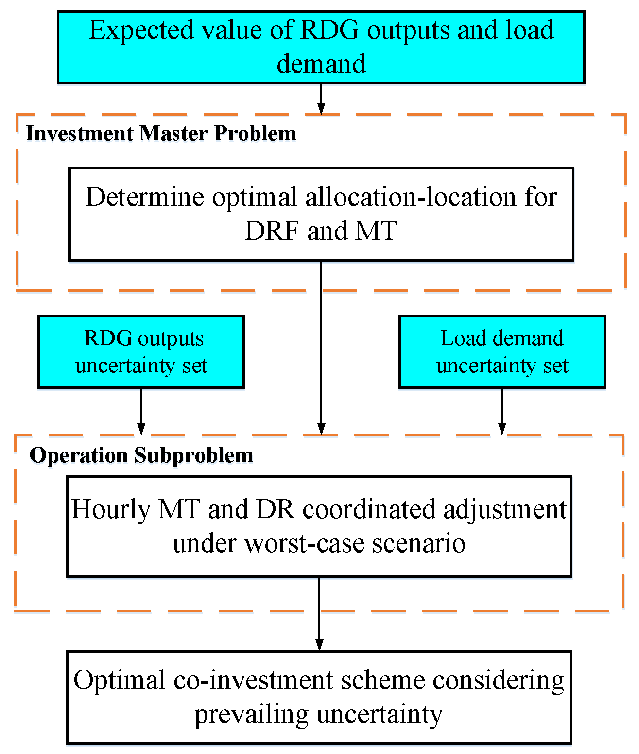
4. Solution Algorithm

4.1. Compact Formulation and Duality
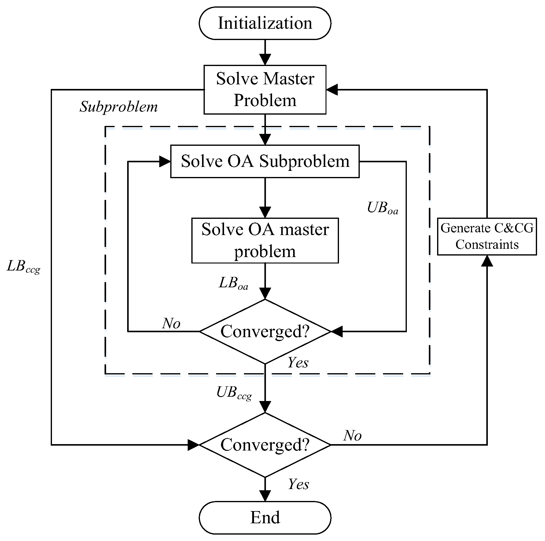
The compact form of the proposed model is written as below:
m i n x a T x + m a x u m i n y , s b T y + e T s + c T u
A x d , x { 0 , 1 }
B y + F s h
G y + I ( u ) x ν
Q y + K ( u ) x + D u = ω
u U
According to their specialty, all the binary variables are grouped in x (i.e., x = {αj, βj}). Moreover, the second-stage variables are divided into operation variable y and slack variable s. Operation variables include DGs and Static Var Compensators (SVCs )outputs Pdg and Qsvc, adjusted DR program participation dk, and uncontrollable BFM variables P, Q, V. The uncertain variables, including wind power, PV outputs P n , t w t , p v , and deviation rate R j , t d of load demand are expressed as u. Otherwise, the constraints (5a)–(5h) and (6t) for x can be grouped into (9b), and the operation constraints (9c)–(9e) can account for (6a)–(6s) and (6u)–(6w). It is noted the I(u) and K(u) are the coefficient matrix of x, and include the uncertainty variables according to (6a)–(6q). The uncertainty sets (7a)–(7c) are sorted in (9f).
The optimization problem (9a)–(9f) can be divided into two stages. Mathematically, with a given u* generated from sub-problem, the master problem can be driven from (9) and become a mix-integer linear program (MILP), which can be directly solved by a commercial solver. Hence, an optimal solution (x*, λ*) can be obtained, in which λ* denotes the value of second-stage objective function value. With these decision variables x*, the sub-problem becomes a “max-min” bi-level program, which is noted as O(u, x*) in this paper. Due to its strong duality, O(u, x*) is equivalent to the dual problem as follows:
S ( u , x ) = m a x ϕ 1 , ϕ 2 , ϕ 3 , u h T ϕ 1 + ( ν I ( u ) x ) T ϕ 2 + ( ω K ( u ) x D u ) T ϕ 3 + c T u
Φ D C = { B T ϕ 1 + G T ϕ 2 + Q T ϕ 3 b
F T ϕ 1 e T
ϕ 1 , ϕ 2 0 }
u U
where {ϕ1, ϕ2, ϕ3} are the dual variable vectors for constraints (9c)–(9e).

4.2. Algorithm

The CCG algorithm is an efficient decomposition algorithm for two-stage robust optimization [29]. Thus, a two-level algorithm is proposed in this subsection, in which the CCG algorithm is adopted in the outer level and the inner level uses an OA algorithm [30] to solve the bilinear problem in (10). The procedure of the proposed algorithm is given in following steps, with a defined convergence index ε:
The outer CCG algorithm is given as:
(1)
Initialize LBccg = −∞, UBccg = +∞, g = 0 and set the sub-problem solution set soa = ∅.
(2)
Solve the master problem, obtain the optimal solution ( x g + 1 , λ g + 1 ), and let LBccg = max{LBccg, aT x g + 1 + λ g + 1 }
(3)
Solve the sub-problem with fixed first stage decision variables and add u g + 1 to soa. Update UBccg = min{UBccg, aT x g + 1 + O( u g + 1 , x g + 1 )}
(4)
Check the convergence index. Return x g + 1 and stop if (UBccg LBccg)/LBccg ≤ Δ. Otherwise, let g = g + 1 and go to step 2.
The inner OA algorithm is given as,
(1)
Initialize LBoa = −∞, UBoa = +∞, m = 1. Fix the first-stage decision variables. Find an initial u i
(2)
Solve the OA sub-problem S ( u m , x ) , Let { ϕ 1 , m , ϕ 2 , m , ϕ 3 , m } be the optimal solution. Set LBoa = S ( u m , x )
(3)
Linearize the bilinear terms at ( u m , ϕ 1 , m , ϕ 2 , m , ϕ 3 , m ), as follows:
( u , ϕ 1 , ϕ 2 , ϕ 3 ) = m a x ϕ 1 , ϕ 2 , ϕ 3 , u ( I ( u ) x ) T ϕ 2 + ( I ( u ) x I ( u ) x ) T ϕ 2 + ( K ( u ) x D u ) T ϕ 3 + ( K ( u ) x + D u K ( u ) x D u ) T ϕ 3
(4)
Solve the OA master problem, which is the linearized version of the second stage problem, defined as below:
Z ( u m , ϕ 1 , m , ϕ 2 , m , ϕ 3 , m ) = m a x ϕ 1 , ϕ 2 , ϕ 3 , u h T ϕ 1 + ν T ϕ 2 + w T ϕ 3 + c T u + ω
s . t . ω χ ( u , ϕ 1 , ϕ 2 , ϕ 3 ) , χ = 1 , , m
u U
ϕ 1 , ϕ 2 , ϕ 3 Φ D C
Let { u m + 1 , ϕ 1 , m + 1 , ϕ 2 , m + 1 , ϕ 3 , m + 1 } be the optimal solution. Set LBoa = Z ( u m + 1 , ϕ 1 , m + 1 , ϕ 2 , m + 1 , ϕ 3 , m + 1 )
(5)
Check the inner-level convergence. Return u m + 1 and stop if (UBoa − LBoa)/LBoaΔ. Otherwise, let m = m + 1 and go to step 2.
The general framework of the algorithm is described in Figure 3.

5. Case Studies

In this section, the proposed framework and methodology were tested on the modified IEEE 33-node distribution system. All the computational tasks were implemented with a Yalmip toolbox in MATLAB (R2016a, MathWorks, Natick, MA, USA) on a 2.4 GHz personal computer with 8 GB of RAM, using Gurobi as the MILP solver (7.0.1, Gurobi Optimization, Inc., Houston, TX, USA). The optimality gap was set as 10−3.

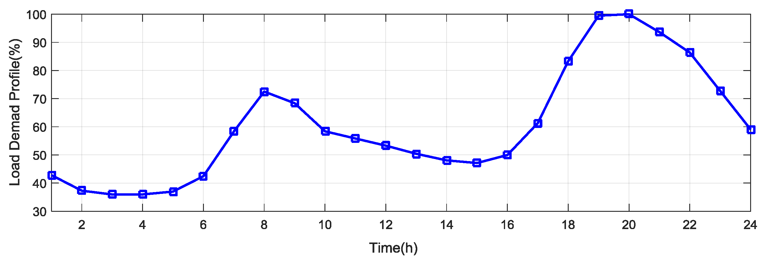
5.1. Modified IEEE 33-Node Distribution Network

The dataset of the modified test system can be obtained from [31].The total peak load demand and capacity of lines were five times of their original given values. The required voltage violation range ε was set as 0.05 (p.u.). The 24-h load demand profile (percentages of daily peak load, shown in Figure 4) were obtained from [32], and they were multiplied by the peak load to determine the expected daily load demand profile. In addition, the electricity price (Prj,t) was assumed to be time-varying, following the change of a 24-h load demand profile, with its peak value set as 50$/MWh. The price to purchase energy from the main grid (Prin) was assumed to be equal to Prj,t, and the price to sell energy to the main grid (Prout) was set as 20% of Prin. Other parameters for describing the renewables and SVCs are listed in Table 1.
In this paper, electricity price was linearized stepwise, with ten-piece segments used in [13] to approximate the price elastic demand curve in (2a). Furthermore, the inelastic demand at each node was set as 80% of the actual demand, and the upper bound of total demand was equal to 120%. Accordingly, Table 2 shows the parameters for various costs in this case study, which were obtained from [16,33]. The discrete increment of DG was set to be 10 kVA in this case study. The interest rate z was set as 3%, and the planning horizon was set as 20 years, respectively.

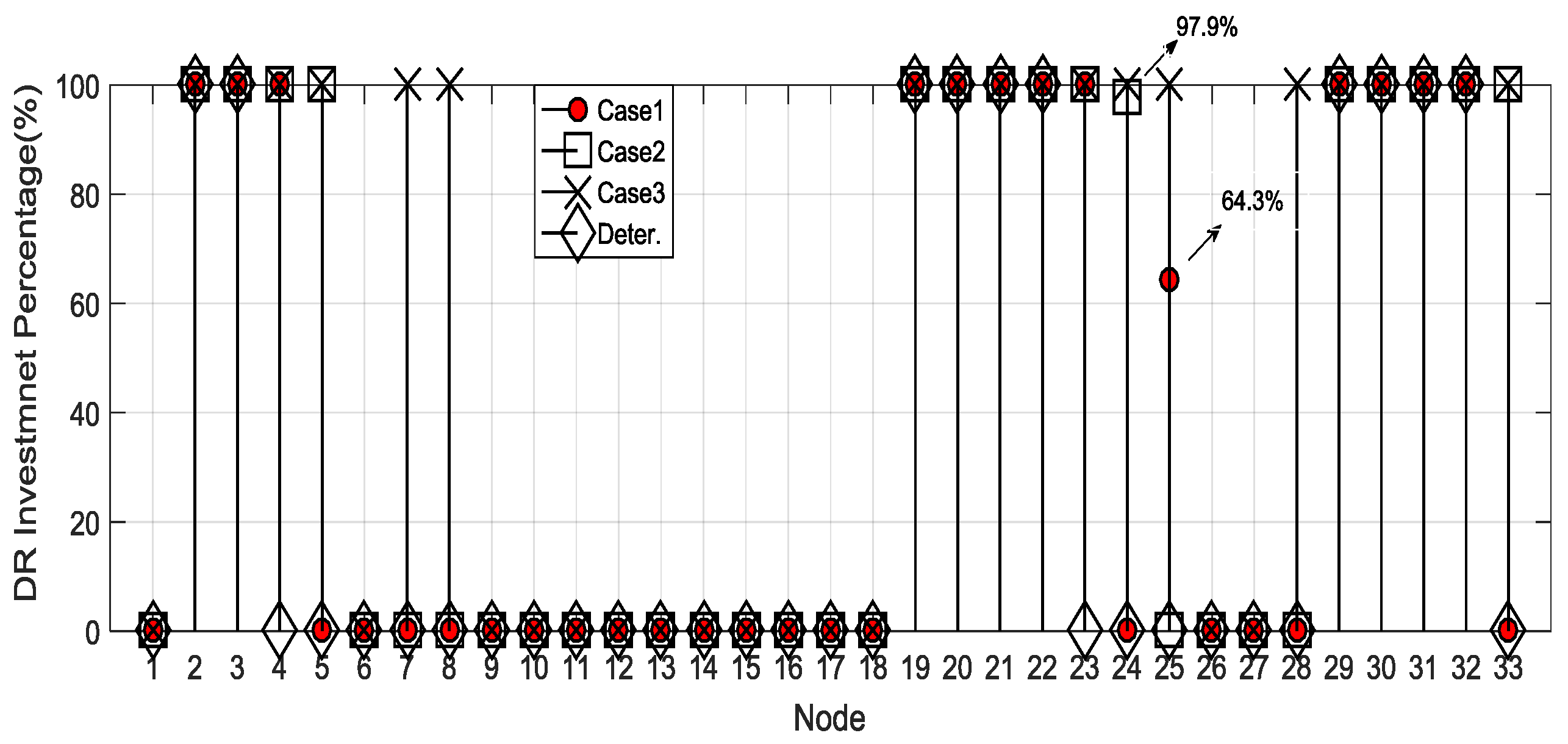
5.2. First-Stage Co-Investment Scheme in a Different Uncertainty Set

We set Case 1 as the base case, in which the uncertainty budget is given in Table 3. To comprehensively illustrate the co-investment scheme in different uncertain budgets of renewable energy, three cases were defined with different Γ l o w w t , p v / Γ u p w t , p v . Table 4 depicts the investment of DG in each case. It can be observed that the locations of DGs are similar, but the sizes installed in the particular locations are relatively different. That is mainly because the DG location depends on the topology, which remains unchanged for all cases, but the DG size depends on the severity of DN operation violation, which is further affected by the uncertainty budget. Figure 5 shows the results of DR investment in three robust optimization-based cases, and one deterministic optimization-based case. It can be observed the DR program investment increases when the uncertainty budget is broadened. Furthermore, Table 5 presents the corresponding investment cost of each case. It is worth noticing that the investment costs for DGs are almost invariant, while the DR investment cost is enlarged with different renewables’ uncertainty budgets. However, considering that DR investment holds a small proportion of the co-planning cost, a slight increase of total investment cost can help the system to hedge against variation of renewable energy sources, which reveals the economic benefit of the DR program investment.

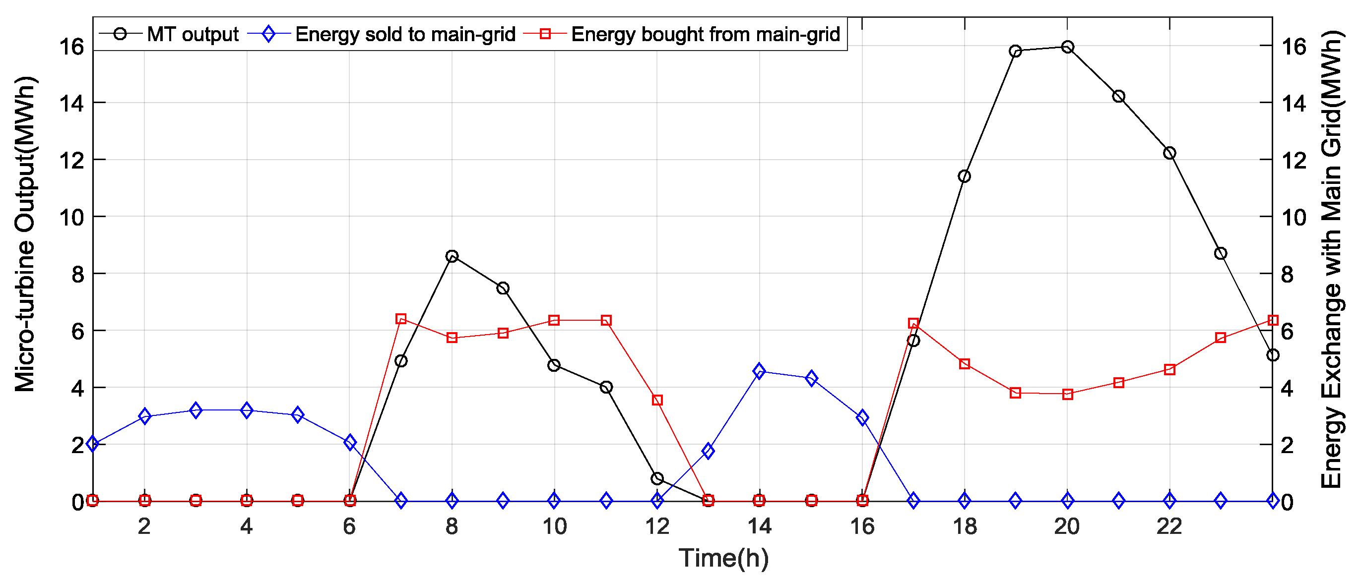
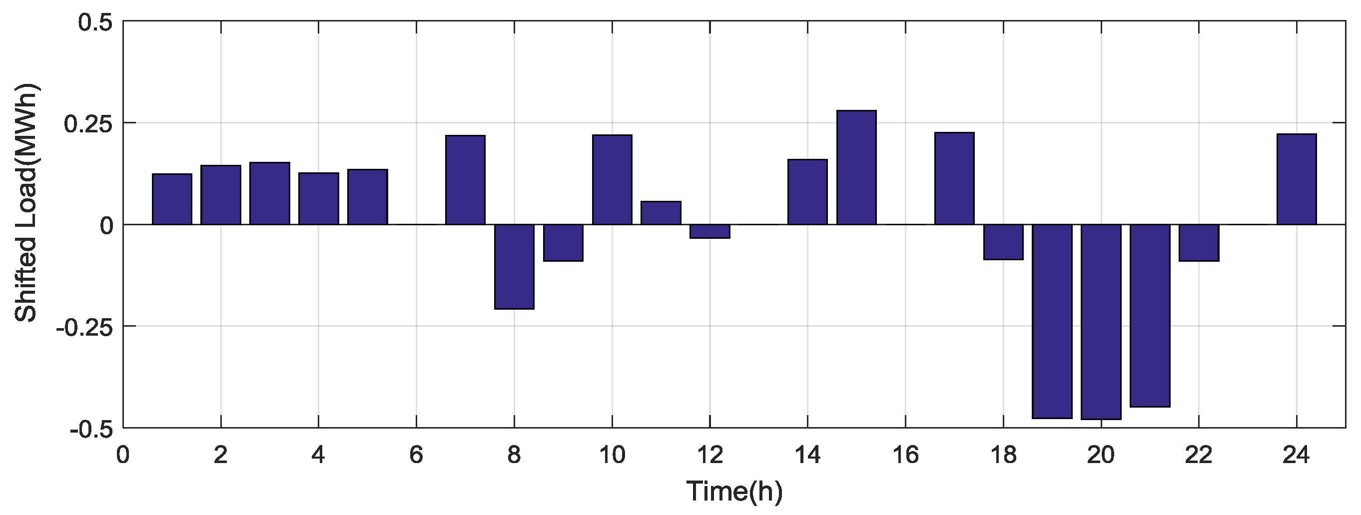
5.3. Second-Stage Operation Result

After the first-stage optimal DR and DG allocation location is given, the worst-case scenario is found based on the second-stage operation strategy. The total hourly DG output and the hourly energy transaction with the main grid in Case 1 are presented in Figure 6. It can be clearly seen that the DG outputs are high during period from 8:00 to 9:00 and from 19:00 to 23:00. According to the daily load profile shown in Figure 4, this is mainly because the electricity consumption is high and renewable energy is low at these time periods. Specifically, the generation of DGs reach their maximum output between 19:00 and 20:00, when the load demand hits its peak value and renewables reach their lower bound. In this situation, the energy provided by all the DGs and the energy reduced by DR program combined is not sufficient to fulfill the peak load, and thus the DN needs to buy energy from external grid. Besides, during the period from 24:00 to 6:00 and from 13:00 to 16:00, when the wind and solar energy is supposed to be abundant and the load demand is low and stable, the DN sells energy to the main grid and the DGs are not committed on.
Figure 7 displays the load shifting under DR-enabled nodes in Case 1, where the load shifting is defined as the difference between DR load and expected demand. It can be seen that the load demand is enlarged between 14:00 and 15:00, when electricity price is low but the wind power and solar energy are more than enough to supply the low power demand. Similarly, the DR is also fitted up to augment the electricity consumption between 24:00 and 6:00, due to the abundant wind power and low energy price. When the wind energy generation is insufficient, and the energy purchased from external grid is expensive, the electricity consumption is reduced from 8:00 to 9:00 and 18:00 to 22:00, respectively. Thus, it can be found that the coordinated operation of DR program and DG can effectively accommodate the uncertainties of renewables and load.

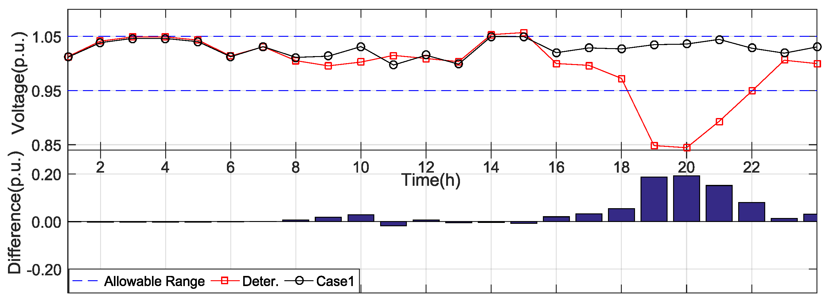
5.4. Voltage Profile with Different Demand Response Ability

To verify the robustness in maintaining system security, the worst-case scenario obtained in Case 1 is implemented, using both the proposed model and the deterministic model. Figure 8 depicts the 24-h voltage profit for the critical node in the test system. It can be observed that severe voltage issues, including voltage over-drop and over-rise, emerge in deterministic results at 15:00 and from 19:00 to 21:00, which leads a large penalty cost. Nevertheless, with the co-investment decision in Case 1 and the proposed operation strategy, the voltage fluctuations in the worst-case scenario are maintained within the acceptable range and the voltage violations are significantly diminished. Again, the proposed co-planning scheme and operation strategy is proved to be able to accommodate the renewable energy both economically and robustly.

5.5. Statistical Feasibility Check

To verify the robustness in addressing various scenarios, the proposed model was tested with 1079 scenarios, randomly generated from a three-year dataset of wind power, PV, and load demand in [32,34,35]. The deterministic model was also implemented as benchmark. Table 6 shows the statistic results of the simulations. As seen from the results, the merits and the defects of the proposed model were validated from different aspects. The average operation cost of the proposed model at $28,420.20 was larger than that of deterministic model, at $26,478.56. Using the proposed model, more DGs were invested, and thus the fuel cost increased accordingly. However, the average energy transaction cost was considerably reduced. The DN revenue in the proposed model slightly decreased as more demand load joined the DR program. Besides, the average maximal voltage violation rate was significantly reduced, from 7.546% to 0.006%. As a result, the average penalty cost was also considerably reduced. It should be noticed that the probability that the proposed model outperforms the deterministic model in total second-stage cost and voltage security is 95.85% and 98.99% respectively, which indicates the robustness of proposed model in maintaining the DN operations.

5.6. Modified IEEE 123-Node Distribution Network

To demonstrate the scalability and effectivity of the proposed framework, a modified IEEE 123-node DN in [36] was also used as a test system, which additionally included eight 1.1 MW WT, 0.5 MW PV, and 1.5 MVAR SVC in the same locations, which were connected at nodes 6, 37, 42, 56, 62, 69, 86 and 114. The 24-h load demand profile was the same as the 33-node system, and the total peak load demand and capacity of lines were five times of their original given values. The other parameters were the same as Section 5.1.
Table 7 shows the co-planning scheme in three robust optimization-based cases and one deterministic optimization-based case, in which the uncertainty sets were the same as in Section 5.2. Furthermore, Table 8 presents the corresponding investment cost of each case. In general, it could be observed that results of DGs and DR investment showed the same trend with the results in the 33-node test system, which verifies the efficiency and scalability of the proposed framework.

6. Conclusions

This paper proposes a DRF and DG co-investment model to determine the optimal capacity and location of demand response and DG. A robust, optimization-based two-stage model was adopted to accommodate the uncertainties of renewables and load demand. The price-sensitive demand was modeled with modified PEDR, where both inelastic and elastic demand was taken into account. In the proposed model, the overall cost was optimized, taking into consideration the first-stage investment decision, as well as the hourly DG and DR coordinated operation in second-stage operation. The customer bills, total energy supply, and operation regulations were considered to motivate the electricity end users to participate in the DR program. Finally, a modified CCG/OA algorithm was employed to solve the proposed two-level programming problem. Case studies demonstrate the effectiveness of the proposed model from aspects of economic and security operations. With the aid of the proposed model, not only is the operation violation of the DN alleviated, but the system cost is also minimized.

Acknowledgments

This work was partially supported by The Hong Kong Polytechnic University under Grant No. G-SB68, and Research Grants Council of Hong Kong, China under Theme Based Research Scheme Grant No. T23-407/13N and T23-701/14N.

Author Contributions

This article has five authors: Yi Yu, Zhao Xu, and Xishan Wen conceived and designed the research method; Yi Yu, Jian Zhao and Jiayong Li performed the numerical experiment; Yi Yu and Jian Zhao analyzed the data; and Yi Yu wrote the paper.

Conflicts of Interest

The authors declare no conflict of interest.

Nomenclature

A. Indices and Sets
t/TIndex/set of time slots
j/JIndex/set of DN nodes
i/ΩjIndex/set of child nodes of node j
d/DIndex of load demand
dg/DGIndex of DG
n/Nwt, NpvIndex/set of the wind power/solar energy
sv/NsvIndex/set of automatic voltage regulators (SVCs)
B. Parameters
CClcs/CCamiLoad control switch/advanced metering infrastructure procurement and installation cost
CCinc/CCeduFinancial incentive and education cost for DR program
CCdgDG procurement and installation cost
εCapital recovery factor for day-based cost
θWeighting factor for transferring yearly cost to daily cost
NsMaximum number of nodes with DRF and DG installation
B j m a x Maximum increment in size of DG at j
C d g o m / C w t o m / C p v o m Operation and maintenance cost of DG/WT/PV generations
C d g f l Fuel cost of DG
Prin/ProutElectricity price for buying/selling energy to/from the main grid
P r j , t k Electricity price at step k in the linearized PEDR model at j,t
l j , t k kth length in the linearized PEDR curve at j,t
P j , t s d / Q j , t s d Expected load demand from statistic data at j,t
D0/D1Coefficient for inelastic part and maximum of actual load demand at j,t
P m i n s u b / P m a x s u b Lower/upper bound of power flow into/from substation
P i j c a p Capacity of the DN line ij
Q m a x s v g Maximum SVC output at sv, t
P i j c a p Capacity of the DN line ij
Q m a x s v g Maximum SVC output at sv, t
P m e a n , n , t w t , p v Mean value of WT/PV output
μ l o w , j , t d / μ u p , j , t d Lower/upper bound of load demand rate at j,t (% of expected demand)
μ l o w , n , t w t , p v / μ u p , n , t w t , p v Lower/upper bound of WT/PV output rate at n,t (% of expected output)
rij/xijResistance/reactance of DN line ij
V0Voltage reference value, set as 1.0 p.u.
σAllowable value of voltage fluctuation
Γ l d , w t , p v / Γ p d , w t , p v Uncertainty budget of load demand/wind power/solar energy
C. Variables
α j d r / α j d g Binary variable indicating if DRF/DG is installed at j
β j d r DR investment percentage indicating the load demand rate with DR ability (% of the peak load) at j
β j , b d g Integer variable indicating bth increments in size of DG at j
Pj,t/Qj,tActive/reactive power flow at j,t
Vj,tVoltage at j,t
P j , , t d g / Q s v , t s v g DG/SVC output at j/sv, t
d j , t k Auxiliary variable introduced at kth step in PEDR model at j,t
h j , t d Actual load demand at j,t
r j , t d Electricity payment of load demand with DR program at j,t
R j , t d Uncertain variation rate of load demand at j,t
S j , t u v / S j , t l v ,Slack variables of voltage violation at j,t
S j i , t u c a p / S i j , t l c a p Slack variables of line capacity limitation at ij,t
S t u s u b / S t l s u b Slack variables of substation capacity limitation at j,t

References

  1. Pepermans, G.; Driesen, J.; Haeseldonckx, D.; Belmans, R.; D’haeseleer, W. Distributed generation: Definition, benefits and issues. Energy Policy 2005, 33, 787–798. [Google Scholar] [CrossRef]
  2. Twidell, J.; Weir, T. Renewable Energy Resources, 3rd ed.; Routledge: New York, NY, USA, 2015. [Google Scholar]
  3. Xu, Z.; Xue, Y.; Wong, K.P. Recent advancements on smart grids in China. Electr. Power Compon. Syst. 2014, 42, 251–261. [Google Scholar] [CrossRef]
  4. Ackermann, T.; Andersson, G.; Söder, L. Distributed generation: A definition. Electr. Power Syst. Res. 2001, 57, 195–204. [Google Scholar] [CrossRef]
  5. Siano, P.; Mokryani, G. Probabilistic assessment of the impact of wind energy integration into distribution networks. IEEE Trans. Power Syst. 2013, 28, 4209–4217. [Google Scholar] [CrossRef]
  6. Catalão, J.P.S. Smart and Sustainable Power Systems: Operations, Planning, and Economics of Insular Electricity Grids; CRC Press: Boca Raton, FL, USA, 2015. [Google Scholar]
  7. Tonkoski, R.; Turcotte, D.; El-Fouly, T.H. Impact of high PV penetration on voltage profiles in residential neighborhoods. IEEE Trans. Sustain. Energy 2012, 3, 518–527. [Google Scholar] [CrossRef]
  8. Su, C.L.; Kirschen, D. Quantifying the effect of demand response on electricity markets. IEEE Trans. Power Syst. 2009, 24, 1199–1207. [Google Scholar]
  9. Medina, J.; Muller, N.; Roytelman, I. Demand response and distribution grid operations: Opportunities and challenges. IEEE Trans. Smart Grid 2010, 1, 193–198. [Google Scholar] [CrossRef]
  10. Palensky, P.; Dietrich, D. Demand side management: Demand response, intelligent energy systems, and smart loads. IEEE Trans. Ind. Inform. 2011, 7, 381–388. [Google Scholar] [CrossRef]
  11. Bitaraf, H.; Rahman, S. Reducing curtailed wind energy through energy storage and demand response. IEEE Trans. Sustain. Energy. 2018, 9, 228–236. [Google Scholar] [CrossRef]
  12. Bukhsh, W.A.; Zhang, C.; Pinson, P. An integrated multiperiod opf model with demand response and renewable generation uncertainty. IEEE Trans. Smart Grid 2016, 7, 1495–1503. [Google Scholar] [CrossRef]
  13. Zhao, C.; Wang, J.; Watson, J.P.; Guan, Y. Multi-stage robust unit commitment considering wind and demand response uncertainties. IEEE Trans. Power Syst. 2013, 28, 2708–2717. [Google Scholar] [CrossRef]
  14. Zhang, C.; Xu, Y.; Dong, Z.Y.; Wong, K.P. Robust coordination of distributed generation and price-based demand response in microgrids. IEEE Trans. Smart Grid. 2017. [Google Scholar] [CrossRef]
  15. Li, X.R.; Yu, C.W.; Xu, Z.; Luo, F.J.; Dong, Z.Y.; Wong, K.P. A multimarket decision-making framework for GENCO considering emission trading scheme. IEEE Trans. Power Syst. 2013, 28, 4099–4108. [Google Scholar] [CrossRef]
  16. US Department of Energy. Benefits of Demand Response in Electricity Markets and Recommendations for Achieving Them; US Department of Energy: Washington, DC, USA, 2006.
  17. Torriti, J.; Hassan, M.G.; Leach, M. Demand response experience in Europe: Policies, programmes and implementation. Energy 2010, 35, 1575–1583. [Google Scholar] [CrossRef]
  18. Saele, H.; Grande, O.S. Demand response from household customers: Experiences from a pilot study in norway. IEEE Trans. Smart Grid 2011, 2, 102–109. [Google Scholar] [CrossRef]
  19. Pourmousavi, S.A.; Patrick, S.N.; Nehrir, M.H. Real-time demand response through aggregate electric water heaters for load shifting and balancing wind generation. IEEE Trans. Smart Grid 2014, 5, 769–778. [Google Scholar] [CrossRef]
  20. Bradley, P.; Leach, M.; Torriti, J. A review of the costs and benefits of demand response for electricity in the UK. Energy Policy 2013, 52, 312–327. [Google Scholar] [CrossRef]
  21. Faruqui, A.; Harris, D.; Hledik, R. Unlocking the €53 billion savings from smart meters in the eu: How increasing the adoption of dynamic tariffs could make or break the EU’s smart grid investment. Energy Policy 2010, 38, 6222–6231. [Google Scholar] [CrossRef]
  22. Thimmapuram, P.R.; Jinho, K.; Botterud, A.; Youngwoo, N. Modeling and Simulation of Price Elasticity of Demand Using an Agent-Based Model. In Proceedings of the 2010 Innovative Smart Grid Technologies (ISGT), Gaithersburg, MD, USA, 19–21 January 2010; pp. 1–8. [Google Scholar]
  23. Wang, X.; McDonald, J.R. Modern Power System Planning; McGraw-Hill Companies: New York, NY, USA, 1994. [Google Scholar]
  24. Afgan, N.H.; Carvalho, M.G.; Hovanov, N.V. Energy system assessment with sustainability indicators. Energy Policy 2000, 28, 603–612. [Google Scholar] [CrossRef]
  25. Baran, M.; Wu, F.F. Optimal sizing of capacitors placed on a radial distribution system. IEEE Trans. Power Deliv. 1989, 4, 735–743. [Google Scholar] [CrossRef]
  26. Baran, M.E.; Wu, F.F. Optimal capacitor placement on radial distribution systems. IEEE Trans. Power Deliv. 1989, 4, 725–734. [Google Scholar] [CrossRef]
  27. Yeh, H.G.; Gayme, D.F.; Low, S.H. Adaptive var control for distribution circuits with photovoltaic generators. IEEE Trans. Power Syst. 2012, 27, 1656–1663. [Google Scholar] [CrossRef]
  28. Zhang, G.; Wu, Y.; Wong, K.P.; Xu, Z.; Dong, Z.Y.; Iu, H.H.C. An advanced approach for construction of optimal wind power prediction intervals. IEEE Trans. Power Syst. 2015, 30, 2706–2715. [Google Scholar] [CrossRef]
  29. Zeng, B.; Zhao, L. Solving two-stage robust optimization problems using a column-and-constraint generation method. Oper. Res. Lett. 2013, 41, 457–461. [Google Scholar] [CrossRef]
  30. Duran, M.A.; Grossmann, I.E. An outer-approximation algorithm for a class of mixed-integer nonlinear programs. Math. Program. 1986, 36, 307–339. [Google Scholar] [CrossRef]
  31. Ding, T.; Li, F.; Li, X.; Sun, H.; Bo, R. Interval radial power flow using extended distflow formulation and krawczyk iteration method with sparse approximate inverse preconditioner. IET Gener. Transm. Distrib. 2015, 9, 1998–2006. [Google Scholar] [CrossRef]
  32. Commercial and Residential Hourly Load Profiles for All TMY3 Locations in the United States. Available online: https://openei.org/doe-opendata/dataset/commercial-and-residential-hourly-load-profiles-for-all-tmy3-locations-in-the-united-states (accessed on 21 October 2017).
  33. Zou, K.; Agalgaonkar, A.P.; Muttaqi, K.M.; Perera, S. Distribution system planning with incorporating dg reactive capability and system uncertainties. IEEE Trans. Sustain. Energy. 2012, 3, 112–123. [Google Scholar] [CrossRef]
  34. NREL. Available online: https://www.nrel.gov/rredc/wind_resource (accessed on 20 June 2017).
  35. Hong Kong Observatory. Available online: http://www.hko.gov.hk (accessed on 8 July 2017).
  36. Zhao, J.; Wang, J.; Xu, Z.; Wang, C.; Wan, C.; Chen, C. Distribution network electric vehicle hosting capacity maximization: A chargeable region optimization model. IEEE Trans. Power Syst. 2017, 32, 4119–4130. [Google Scholar] [CrossRef]
Figure 1. Two-stage, robust co-planning framework.
Energies 11 00354 g001
Figure 2. Step-wise function approximation of PEDR curve.
Energies 11 00354 g002
Figure 3. The framework of the algorithm.
Energies 11 00354 g003
Figure 4. 24-h Load Demand Profile.
Energies 11 00354 g004
Figure 5. Demand response (DR) Investment Scheme in different cases.
Energies 11 00354 g005
Figure 6. 24-h second-stage operation.
Energies 11 00354 g006
Figure 7. Shifted load demand at second-stage operation.
Energies 11 00354 g007
Figure 8. Voltage profile of critical nodes in different cases.
Energies 11 00354 g008
Table 1. Simulation data for WT, PV and SVC.
LocationCapacity
WT (MW)PV (MW)SVC (MVar)
173.6751.1253.250
192.6251.5753.250
242.6250.6753.250
331.5751.1253.250
Table 2. Parameters for corresponding costs.
ParameterValueParameterValue
CClcs96$/KWh C p v o m 0.006$/KWh
CCami100$ C d g f l 0.33$/KWh
CCdg2293$/KWhCCinc9.6$/unit
C d g o m 0.02$/KWhCCedu9.6$/unit
C w t o m 0.008$/KWhCCpena1000$/p.u.
Table 3. Uncertainty set budget.
BudgetsμlowμupΓlowΓup
WT0.201.800.901.10
PV0.202.000.901.10
Load demand0.901.100.981.02
Table 4. Distributed generators’ deployments in different cases.
Case Γ l o w w t , p v Γ u p w t , p v Size (MW)Location (Node)
10.901.101.0025
1.109
1.5032
2.5012, 14, 24, 29, 33
20.801.200.9024
1.159
1.5529
2.5013, 14, 25, 30, 33
30.701.300.1231
0.4725
0.5010
2.5012, 13, 24, 29, 30, 32
Deter.--0.3532
0.8110
1.8425
2.50 13, 29, 30
Table 5. Investment cost for a co-planning scheme in different cases.
CaseCdr ($)Cdg ($)Cinv ($)
1185.726796.826982.55
2214.126796.837010.94
3317.836788.387106.21
Deter.135.014432.714567.22
Table 6. Statistical feasibility check results.
Case C o p e a v r ($) C a n d a v r ($) C r e v a v r ($) C p e n a a v r ($) R m a x v , a v r (%) R b e a t c (%) R b e a t v m a x (%)
128420.204137.84338.0019.740.00695.8998.99
Deter26478.564472.54341.06290607.847.546
C o p e a v r : Average operation cost C a d n a v r : Average energy transaction cost. C r e v a v r : Average revenue; C p e n a a v r : Average penalty cost. R m a x v , a v r : Average maximal voltage violation rate; R b e a t c : Rate of proposed model beat Deter in total second-stage cost; R b e a t v m a x : Rate of proposed model beat Deter in maximal voltage violation rate.
Table 7. Co-planning scheme in different cases of a 123-node test system.
CaseDGs DeploymentsDR Investment
Size (MW)Location (Node)Percentage (%)Location (Node)
10.031511007, 9, 11, 10, 19, 20, 28, 33, 29, 30
37, 42, 45, 47, 46, 48, 49, 50
51, 151, 55, 56, 60, 62, 63, 64
65, 68, 69, 70, 71, 76, 77, 86
79, 80, 82, 83, 87, 88, 94, 95
98, 99, 35, 1, 52
0.22108
0.27450, 80
0.3646
0.6082
0.8265, 91
1.4379, 49
2.5093
20.10341007, 9, 11, 10, 19, 20, 28, 33, 29, 30
37, 42, 45, 46, 47, 48, 49, 50, 51
53, 55, 56, 60, 62, 63, 64, 65, 68
69, 70, 71, 76, 77, 86, 79, 80, 82
82, 83, 87, 88, 94, 95, 98, 99
100, 109, 113, 35, 1, 52
0.1771
0.2065
0.4345
0.6444
0.8782
1.2193
2.4179
2.5089
30.071081007, 9, 11, 10, 19, 20, 28, 33, 29, 30
37, 42, 45, 47, 46, 48, 49, 50, 51
53, 55, 56, 60, 62, 63, 64, 65, 68
69, 70, 71, 76, 77, 86, 79, 80, 82, 83, 87
88, 94, 95, 98, 99, 100, 109, 111, 112
113, 114, 35, 1
0.17450
0.25151
0.2745
1.1487
1.8566
2.5083, 93
Deter.0.22881007, 9, 11, 10, 19, 20, 28, 33
30, 37, 48, 50, 87, 88, 94, 95
35, 1
0.4166
1.1082
2.5093
Table 8. Investment cost for a co-planning scheme in a different case of a 123-node test system.
CaseCdr ($)Cdg ($)Cinv ($)
1348.583693.934042.51
2365.243693.934059.17
3377.383693.934071.31
Deter.157.652427.412585.06

