Article

Hydro-Thermal-Wind Generation Scheduling Considering Economic and Environmental Factors Using Heuristic Algorithms

by
Suresh K. Damodaran
1,* and
T. K. Sunil Kumar
2
1
Department of Electrical Engineering, Government Engineering College, Trichur 680009, India
2
Department of Electrical Engineering, National Institute of Technology Calicut, Kerala 673601, India
*
Author to whom correspondence should be addressed.
Energies 2018, 11(2), 353; https://doi.org/10.3390/en11020353
Submission received: 3 January 2018 / Revised: 27 January 2018 / Accepted: 30 January 2018 / Published: 2 February 2018

Abstract

:
Hydro-thermal-wind generation scheduling (HTWGS) with economic and environmental factors is a multi-objective complex nonlinear power system optimization problem with many equality and inequality constraints. The objective of the problem is to generate an hour-by-hour optimum schedule of hydro-thermal-wind power plants to attain the least emission of pollutants from thermal plants and a reduced generation cost of thermal and wind plants for a 24-h period, satisfying the system constraints. The paper presents a detailed framework of the HTWGS problem and proposes a modified particle swarm optimization (MPSO) algorithm for evolving a solution. The competency of selected heuristic algorithms, representing different heuristic groups, viz. the binary coded genetic algorithm (BCGA), particle swarm optimization (PSO), improved harmony search (IHS), and JAYA algorithm, for searching for an optimal solution to HTWGS considering economic and environmental factors was investigated in a trial system consisting of a multi-stream cascaded system with four reservoirs, three thermal plants, and two wind plants. Appropriate mathematical models were used for representing the water discharge, generation cost, and pollutant emission of respective power plants incorporated in the system. Statistical analysis was performed to check the consistency and reliability of the proposed algorithm. The simulation results indicated that the proposed MPSO algorithm provided a better solution to the problem of HTWGS, with a reduced generation cost and the least emission, when compared with the other heuristic algorithms considered.

1. Introduction

The role of optimal generation scheduling of a thermal-renewable power generation system aiming economic and environmental benefits is vital in the current scenario of increasing power demand, escalating the fuel price and high pollution rate. The optimal generation scheduling of a hydro-thermal-wind system aims to distribute the power demand among the generating plants in such a way that the net energy cost and emission of pollutants are minimised, while satisfying the various constraints of power plants. Earlier, the combined operation of hydro-thermal plants was successfully scheduled to reduce the fuel cost, as well as the emission of pollutants. Now, with the development and readiness of new and cost-effective technologies, the penetration of wind power plants in the energy sector has become significant, necessitating its inclusion in the scheduling process. But, research publications describing the optimal generation scheduling of such hybrid energy sources are scanty.
The HTWGS is a non-linear optimization problem with two conflicting objectives. The first approach for solving the HTWGS problem is adopting calculus-based solution techniques (conventional method) such as linear programming [1], dynamic non-linear programming [2], lagrangian relaxation [3], and differential dynamic programming [4], etc. These methods are iterative techniques, containing composite mathematical expressions and long computational steps. Also, they have a limited space to address discrete and non-differentiable problems. The second approach is to adopt heuristic optimization methods which mimic the natural behaviour of certain things or physical phenomena of certain items. This approach gained wide popularity due to the easiness of implementation, adaptability in searching for the best solution, and ability to address non-linear optimization problems. It can be broadly classified as, evolutionary algorithms, swarm intelligence based methods, and algorithms based on the principle of other natural phenomena.
A comprehensive review of short-term hydrothermal scheduling (STHTS) using different classes of heuristic algorithms has been elaborated in [5]. The Genetic Algorithm is applied to generate optimal generation scheduling of a short-term hydrothermal system in [6,7]. An evolutionary algorithm is employed for addressing STHTS in [8,9]. Following evolutionary algorithms, swarm intelligence-based optimisation algorithms received wide acceptance due to the lower number of computational steps and control variables involved. One popular algorithm in this category is particle swarm optimization (PSO). In [10], the PSO method was proposed for STHTS of the multi-reservoir cascaded system. The predator prey optimisation (PPO) technique, which is an extended version of PSO, was suggested in [11] as a solution for STHTS. There are several reports on the use of heuristic algorithms to optimize wind-thermal plant scheduling. An artificial bee colony optimization algorithm was employed for emission and economic dispatch on a wind–thermal system in [12]. A modified particle swarm optimization algorithm influenced by the gravitational search method was adopted to effect emission level reduction in [13]. Many other heuristic algorithms based on natural phenomena and the random optimization process such as Harmony search (HS) and JAYA algorithms have been reported. The HS algorithm [14] mimics the improvisation procedure of an orchestra. A solution to STHTS using the HS algorithm was also proposed in [15]. In [16], a newly introduced population-based heuristic algorithm (JAYA algorithm) was applied for optimal power flow solution. The optimal generation scheduling of a hybrid system consisting of hydro-thermal-wind plants has not often been reported in the literature. The intermittent behavior of wind power is the main hurdle in the massive incorporation of wind plants into the hydrothermal system. Many researchers have addressed the unpredictable nature of wind power using fuzzy logic, neural network, and time series analysis, etc. The Weibull distribution function [17] is suitable for modelling wind speed characteristics with minimum parameters. An incomplete gamma function term is used in [18] to illustrate the wind power impact. In [19], the stochastic wind power was considered as a constraint. The fluctuating nature of wind power can be considerably mitigated by the wind-hydro joint operation since hydropower can be altered rapidly. Some of the associated works on HTWGS were described in [20,21,22,23,24]. Security constrained hydrothermal generation scheduling accounting for the discontinuity and uncertainty of wind power is addressed in [20]. But, in this model, the emission of pollutants from the thermal plant is not accounted for. In [21], the NSGA-III technique is used for computing the optimal allocation load among the hydro-thermal-wind power units. In this paper, the thermal power is modelled as a quadratic polynomial where only limited generator constraints are considered. Reference [22] presents a bee colony optimization method for finding short-term economic/environmental HTWGS, incorporating wind power uncertainty, along with non-linear generator constraints, into the approach. A distributionally robust optimization method is proposed in [23] for solving the hydro-thermal-wind economic dispatch problem. In this paper, the S-lemma method is used to incorporate the wind power uncertainty within a confined set. In [24], the spinning reserve was considered and allocated between the hydro-thermal units to mitigate the challenges that occurred due to the uncertain nature of wind power during HTWGS.
This paper investigates the capability of selected algorithms representing different heuristic groups for searching for the optimal solution for HTWGS considering economic and environmental factors. Here, well accepted and suitable mathematical functions were chosen for addressing the generation cost, emission of pollutants, and water discharge. An improvement is proposed to conventional PSO, named as modified particle swarm optimization (MPSO), and employed to obtain hour-by-hour optimal generation scheduling of integrated hydro-thermal-wind power plants. An optimum solution was searched for using the proposed method (MPSO) and four other algorithms (BGA, PSO, IHS, and JAYA) with a trial system consisting of a multi-reservoir cascaded system with four hydro, three thermal, and two wind power plants. The two objective functions dealing within the problem, namely economic and emission, are of a conflicting nature. Therefore, a balanced optimal operating point was searched for by combining the two objectives and treating it as one function by means of a penalty factor. This approach reduced the computational burden and provided a better compromised solution. A comparison of the results obtained from the various algorithms used has been presented. Among the algorithms employed, the MPSO method exhibited a better performance and capability for searching for a more optimal solution in the test case.
The paper is organized as follows: Section 2 presents the modeling of hydro-thermal-wind generation scheduling considering economic and emission factors. Section 3 illustrates the outline of GA PSO, HS, and JAYA algorithms. Section 4 gives a short description of the MPSO method. Section 5 presents the computational steps of MPSO. The application of the proposed method in a test system and its results are discussed in Section 6. Section 7 summarizes the conclusions.

2. Hydro-Thermal-Wind Generation Scheduling Considering Economic and Environmental Factors

HTWGS deals with the optimal distribution of power demand among existing generation plants so as to reduce the overall generation cost and pollutant emission during the specified period, satisfying the power limit of plants and water constraint of hydro plants of the integrated generation system.
The total cost of generation comprises the coal cost of the thermal plant and rate of wind power only, since the hydro power cost is independent of generation output. Hence, the objective function to be minimized involves the generation cost of thermal and wind power plants and the emission of pollutants. This problem is basically a nonlinear constrained multi-objective optimization problem. The overall objective function is given by:
M i n i m i z e      C T ( F T , W T , E T )
where CT is the overall cost of the generation of thermal-wind plants, FT is the total fuel cost of thermal plants, WT is the wind power generation cost, and ET is the net pollutant emission from thermal plants.
Subject to a number of equality and inequality constraints as follows:
  • System active power balance:
    j N T P g j , τ + m N H P h m , τ + l N W w l , τ = P D , τ + P L o s s , τ    ( τ = 1 , 2 , , T )
    where NT, NH, and NW are number of thermal, hydro, and wind power plants, respectively; Pgj,τ is the power output of the jth thermal power plant; Phm,τ is the power output of the mth hydro power plant; wl is the power output of the lth wind power plant in the sub-interval τ; PD,τ is the load demand during the sub-interval τ; PLoss is the transmission loss in the sub-interval τ; and T is the scheduling period.
  • The dynamic water balance in the reservoir:
    V h m , τ = V h m , τ 1 + I h m , τ Q h m , τ S h m , τ + l = 1 R u m ( Q h l ( τ t l m ) + S h l ( τ t l m ) )
    where Vhm,τ and Qhm,τ are the storage volume and water discharge rate of the mth hydro plant in the sub-interval τ, respectively; Ihm,τ and Shm are the inflow rate and spillage of the mth hydro power plant in the sub-interval τ, respectively; Rum is the number of upstream hydro plants directly above the mth hydro power plant; and tlm is the water transport delay from reservoir l to m.
  • Initial and final reservoir storage volume:
    V h m , 0 = V h m , b e g i n
    V h m , T = V h m , e n d
    where Vhm,begin and Vhm,end are the initial and final storage volume of mth hydro plant, respectively.
  • Thermal power plant generation limit:
    P g j min P g j P g j max      ( j = 1 , 2 , , N T )
    where P g j min and P g j max are the minimum and maximum power output of the jth thermal power plant, respectively.
  • Hydro power plant generation limit:
    P h m min P h m P h m max        ( m = 1 , 2 , , N H )
    where P h m min and P h m max are the minimum and maximum power output of the mth hydro power plant, respectively.
  • Wind power plant generation limit:
    0 w l w r , l ( l = 1 , 2 , , N W )
    where wrl is the rated power output of the lth wind power plant.
  • Reservoir storage volume and discharge limit:
    V h m , τ min V h m , τ V h m , τ max
    Q h m , τ min Q h m , τ Q h m , τ max
    where V h m , τ min , V h m , τ max and Q h m , τ min , Q h m , τ max are the minimum and maximum reservoir volume and water discharge of the mth hydro plant, respectively.
The hydro units power output is expressed as a function of reservoir volume and head [25] given by:
P h m , τ = C 1 m V h m , τ 2 + C 2 m Q h m , τ 2 + C 3 m V h m , τ Q h m , τ + C 4 m V h m , τ + C 5 m Q h m , τ + C 6 m
where C1m, C2m, C3m, C4m, C5m, and C6m, are the generation coefficients of the mth hydro plant in the sub-interval τ.
In the present work, the multi-objective HTWGS considering economic and emission factors is modified into a single objective optimization problem using a penalty factor [26]. The penalty factor converts the emission to the indirect cost of emission and hence allows treating fuel costs and emission together. Thus, the total cost of the thermal system is the sum of the fuel cost and the indirect cost of emission. The penalty factor hj is given by the equation:
h j = F j ( P g j max ) E j ( P g j max )    $ / l b
Thus, the objective function (1) can be modified as:
M i n i m i z e      C T ( F T + h E T , W T )
The fuel cost function of the thermal plant is expressed as a quadratic function of the real power output [27]. The valve-point effects are taken into account by incorporating a sinusoidal term in the cost function [28]. Consider a grid system with NH hydro, NT thermal, and NW wind power plants. The objective of the problem is to reduce the energy cost of the hydro-thermal-wind system through optimal generation scheduling considering economic and emission factors. The fuel cost function of thermal power plant is denoted by:
F T = τ = 1 T j = 1 N T F j ( P g j , τ ) = τ = 1 T j = 1 N T a j P g j , τ 2 + b j P g j , τ + c j + | e j sin ( h j ( P g j min P g j , τ ) ) |
where Fj(Pgj,τ) is the fuel cost function of the jth thermal power plant in the sub-interval τ in $/h. Pgi,τ is the power output of the jth thermal power plant in the sub-interval τ in MW. aj, bj, cj are the fuel cost coefficients and hj, ej are the coefficients of the valve point effect of the jth power thermal plant. P g j min is the minimum power output of the jth thermal plant.
The pollutant emission from a coal-based power plant depends on the power output of that plant.
The total emission of pollutant E can be expressed [22] as:
E T = τ = 1 T j = 1 N T E j ( P g j , τ ) = τ = 1 T j = 1 N T α j P g j , τ 2 + β j P g j , τ + γ j + η j e δ j P g j , τ l b / h
where αj, βj, γj, ηj, and δj are the coefficients of emission of the jth thermal plant.
The total operating cost of a wind-powered generator consists of three components: (a) direct cost, (b) cost for not utilizing existing wind power (underestimation), and (c) overestimation cost [13]. The cost function of a wind generator is formulated as:
W T = τ = 1 T l = 1 N W ( C d , l ( w l , τ ) + C u , l ( W l , a v l w l , τ ) + C o , l ( w l , τ W l , a v l ) )
where Cd,l is the direct cost function of the wind power plant l. wl is the scheduled wind power output of plant l in the sub-interval τ in MW. Cu,l is the penalty cost function for underestimation and Co,l is the penalty cost function for overestimation of the lth wind power plant. Wl,avl is the available power of the lth wind power plant.
Direct cost is involved when the utility is purchasing the power from the wind farm, which is expressed as a linear cost function of actual power usage.
C d , l ( w l , τ ) = d l w l , τ    ( l = 1 , 2 , , N W ;         τ = 1 , 2 , , T )
where dl is the coefficient of direct cost of the lth wind plant.
The underestimation and overestimation of wind power are mainly due to the uncertainty involved in the available wind power. The power output of a wind turbine depends on the blowing strength of the wind, which relies on many environmental parameters. Hence a reliable and accurate prediction of wind energy is difficult. In this paper, the uncertain nature of the wind generation is accounted for by a probability distribution function. The wind speed frequency distribution can supply a clear-cut picture about the wind speed pattern of a given location. Then, a proper statistical function can be fitted to express the wind speed distribution mathematically.
The penalty cost due to the underestimation of wind energy occurs when the available wind power is more than the predicted power (or actual wind power used), and the system operator should then pay a reasonable amount to the utility to compensate for the wastage of available wind power. Conversely, if the available wind power is less than the expected power (or actual wind power needed), then the system operator should purchase power from alternative sources or the load must be shut down.
The expression for penalty cost corresponding to underestimation and overestimation of wind power presented in [17] was used in this work. The penalty cost function for underestimation of the wind power plant l in the sub-interval τ is expressed as a linear relation showing the difference between available wind power and actual wind power, and is given by:
C u , l ( W l , a v l w l , τ ) = k u , l × w l , τ w r , l , τ ( w w l , τ ) × f W ( w ) d w
where ku,l is the cost coefficient of underestimation of wind power plant l. wr,l,τ is the rated wind power output of the unit l in the sub-interval τ. fW(w) is the probability density function (PDF) of wind power.
The penalty cost function for overestimation of the lth wind power plant in the sub-interval τ is given by:
C o , l ( w l , τ W l , a v l ) = k o , l × 0 w l , τ ( w l , τ w ) × f W ( w ) d w
where ko,l is the cost coefficient of overestimation of the wind power plant l.

Modelling of Wind Speed and Power

The numerical value of the underestimation and overestimation cost is obtained only by assuming a proper statistical function for the wind power output. Weibull distribution is the most popular distribution function, which closely follows the wind speed profile [17,19]. The Weibull probability density function is expressed as:
f υ ( υ ) = ( κ c ) × ( υ c ) ( κ 1 ) × exp ( υ c ) ( κ ) , 0 < υ <
where υ is the wind speed of the given location. κ and c are the shape parameter and scale parameter, respectively.
The wind turbine power output can be mathematically expressed [22] as:
w = { 0 ( υ < υ i n    a n d    υ > υ o ) w r × ( υ υ i n ) ( υ r υ i n ) ( υ i n υ υ r ) w r ( υ r υ υ o )
where w is the power output of the wind turbine (kW or MW); wr is the rated wind power output; and υin, υr, and υo are the cut-in, rated, and cut-out wind speed, respectively.
Thus, the wind turbine power output is a combination of discrete and continuous random variables, ie, wind turbine power output is a discrete random variable between υr and υo and also a continuous random variable between υin and υr.
The Weibull probability distribution function can be obtained for three portions of wind power output, described in Equation (23).
P ( w = 0 ) = P ( υ < υ i n ) + P ( υ > υ o ) = F V ( υ i n ) + ( 1 F V ( υ o ) ) = 1 exp ( υ i n c ) ( κ ) + exp ( υ o c ) ( κ )
and
P ( w = w r ) = P ( υ r υ υ o ) = F V ( υ o ) F V ( υ r ) = exp ( υ r c ) ( κ ) + exp ( υ o c ) ( κ )
The Weibull PDF for the continuous range of wind power output equation is expressed as:
f W ( w ) = κ σ υ i n w r c ( ( 1 + ϕ σ ) × υ i n c ) ( κ 1 ) exp ( ( 1 + ϕ σ ) × υ i n c ) ( κ )
where ϕ = w w r and σ = ( υ r υ i n ) υ i n .

3. Outline of GA PSO, HS, and JAYA Algorithms

3.1. Genetic Algorithm (GA)

GA is an evolutionary-based computation technique that mimics the genetic evolution process. Initially, a set of chromosomes called a population, representing the encoded control parameters, are randomly generated within the search space. The chromosomes are evaluated based on the fitness value derived from the objective function and a new population is generated. The process is repeated until the global optimum point is reached.

3.2. PSO Algorithm

The PSO algorithm is the mathematical simulation of the social behavior of fish schooling or birds’ flocking [26]. The particles constitute a swarm (or group), moving along the solution space searching for an optimal solution. Each particle knows its earlier position (xk), and the best value (pbest) achieved so far. Among the best position of individuals, the optimal value is denoted as gbest. Each individual in the subsequent search attempts to improve the earlier status through the present speed, best position, and gbest.
The following equations are used to compute the new velocity and position of each particle.
v k ( r + 1 ) = C f [ w t   v k ( r ) + c 1 r a n d 1 ( p b e s t k x k ( r ) ) + c 2 r a n d 2 ( g b e s t k x k ( r ) ) ]
x k ( r + 1 ) = x k ( r ) + v k ( r + 1 )
where Cf is the constriction factor; rand1 and rand2 are the random numbers between 0 and 1; v k ( r ) and x k ( r ) are the velocity and position of the kth particle at rth iteration, respectively; wt is the inertia weight; and c1, c2 are the learning factors.
The constriction factor is used to improve the search procedure [28], given by:
C f = 2 | 2 ψ ψ 4 ψ |
where ψ = c1 + c2, ψ > 4.
In order to attain a balance among the local and global search, an inertia weight parameter is introduced, which is given by the equation:
w t = w t max ( w t max w t min ) × r r max
where r is the iteration count and rmax is the maximum number of iterations.

3.3. Harmony Search (HS) Algorithm

The HS algorithm simulates the improvisation procedure of music players to obtain better harmony among the instruments by adjusting the pitches of the instrument [29]. The harmony of instruments resembles the optimization of variables and the improvisation procedure of an orchestra is akin to the local and global search process. A harmony memory (HM) is initialized with randomly generated control variables within the search space. New HM (NHM) is created on the basis of the memory consideration rate (HMCR), pitch alteration (PAR), band width (bw), and random choice. The fitness of each NHM vector is evaluated on the basis of objective function and the corresponding HM vector is replaced, if improvement is exhibited in the NHM vector.
PAR and bw parameters are significant in refining the solution vectors and influence the convergence rate of the algorithm. The Improved Harmony Search algorithm uses a dynamically varying PAR and bw in the search process.

3.4. JAYA Algorithm

JAYA is a population-based optimization algorithm developed by Venkata Rao [30] in 2016. This algorithm does not involve any specific tuning parameters. The optimization process follows the procedure of solution search by shifting towards the optimum solution, avoiding the inferior solution. A population consisting of candidate solution vectors is randomly generated within the search space. The fitness of each candidate solution is evaluated, and the best and worst candidates are identified. Each candidate solution is updated based on the best and worst solutions using Equation (29).
X j , i , k = X j , i , k + r a n d 1 ( X j , b e s t , k | X j , i , k | ) r a n d 2 ( X j , w o r s t , k | X j , i , k | )
where Xj,i,k is the value of the jth variable for the ith candidate during the kth iteration; X j , i , k is the updated value; Xj,best,k and Xj,worst,k are the best and worst solutions, respectively; and rand1 and rand2 are the two random numbers in the range [0, 1].

4. Modified Particle Swarm Optimization (MPSO)

The conventional PSO keeps the randomness of search by maintaining normal random values in the velocity computation equation of each particle. In this case, the velocity calculation of each particle assigns different random values. In the proposed modified particle swarm optimization algorithm, a unique random value is assigned to individual search (pbest) part of the velocity calculation for the population in one iteration. Also, in the global search (gbest) part of the velocity equation, each particle is assigned different random values. This modification shows improvement in the individual search process and is able to explore more optimal solutions compared with conventional PSO.
In MPSO, the equation to update velocity is modified as below.
v k ( r + 1 ) = C f [ w t   v i ( r ) + c 1 r a n d ( r ) ( p b e s t k x k ( r ) ) + c 2 r a n d k ( r ) ( g b e s t k x k ( r ) ) ]
where rand(r) is a uniform random number between 0 and 1 for the rth iteration of the population. randk(r) is the random number of the kth particle in the rth iteration.

5. Solving HTWGS Considering Economic and Emission Factors Using MPSO

The solution technique begins with the illustration of the candidate solution (or decision variables) denoted as the particle. In this study, the decision variables in the optimization process are the thermal power output, the quantity of water discharged, and wind power output (i.e., Pgj,τ, qm, and wn). Thus, each particle carries a solution to these variables and searches for optimal values in the subsequent iteration. Hence, for a scheduling period T, the kth particle xk is expressed as:
x k = [ P g 1 , 1 , j P g 1 , N T , j q 1 , 1 , m q 1 , N H , m w 1 , 1 , l w 1 , N W , l P τ , k , j q τ , k , m w τ , k , l P g T , 1 , j P g T , N T , j q T , 1 , m q T , N H , m w T , 1 , l w T , N W , l ]
The computational steps of the proposed MPSO method are as follows, and the flow chart is shown in Figure 1.
Step 1:
The algorithm starts with initialization of the particles. A uniform random value is chosen between the minimum and maximum limits of the individual decision variables. The initial velocities are also generated in the same way for all the particles.
Step 2:
Compute penalty factor hj for all thermal power plants using Equation (12). These values are constant and hence do not require modification in the iteration process
Step 3:
Calculate the hydro power plant’s output and apply the respective power inequality constraints. If any of the plants violate lower limits, fix the generation to the lower limit. In other words, if any of the plants violate upper limits, fix the generation to the upper limit.
Step 4:
Compute the fuel cost and emission of thermal power plants using Equations (14) and (15).
Step 5:
Compute the wind power generation cost by solving Equations (17)–(19).
Step 6:
Calculate the fitness of the particles, considering all generation costs and equality constraints. Set the present value of each particle as its best position, pbest.
Step 7:
Check for the lowest value of particle best position. Set the value as gbest.
Step 8:
Calculate the updated velocity of each individual by Equation (30).
Step 9:
Update each individual position by Equation (26).
Step 10:
Calculate the new fitness value for each particle. Replace the old pbest value with new one, if the present value shows improvement over the previous value.
Step 11:
Replace the gbest with the lowest value from the new pbest, if the present value shows improvement over the previous value.
Step 12:
Repeat steps 8–11 until the equality constraints fall within a specified tolerance limit or maximum number of iterations reached.
The particle generates the latest gbest, giving the optimum schedule of generation.

6. Simulation Results

In this work, the two conflicting objectives are treated together using the penalty factor. The maximum penalty factor approach has been chosen for combining the fuel cost and emission; it offers an acceptable solution for the problem of emission and fuel cost.
The parameter setting is counted as the main limitation of any heuristic algorithm. Once the parameters are suitably chosen, the algorithm follows the logical pattern and converges to an optimal solution. In this study, the following values are assigned to the control parameters of each algorithm. The range of these parameter values is considered by observing similar published case studies, and the fine turning is done by a trial-and-error process.
MPSO and PSO parameters:
  • Swarm size (population) = 10
  • Learning factors, c1, c2 = 2.05
  • Maximum iterations = 500
  • wtmin = 0.4, wtmax = 0.9
Binary Coded GA parameters:
  • Size of Population = 60
  • Probability of crossover = 0.7
  • Probability of mutation = 0.1
  • Probability of elitism = 0.15
  • Maximum iterations = 500
Harmony Search parameters:
  • Harmony Memory Size (HMS) =10
  • Harmony Memory Consideration Rate (HMCR) = 0.85
  • Pitch Adjustment Rate (PAR): PARmin = 0.2, PARmax = 2
  • Bandwidth (bw): bwmin = 0.45, bwmax = 0.9
JAYA Algorithm parameters:
  • Size of Population = 10
  • Maximum iterations = 500
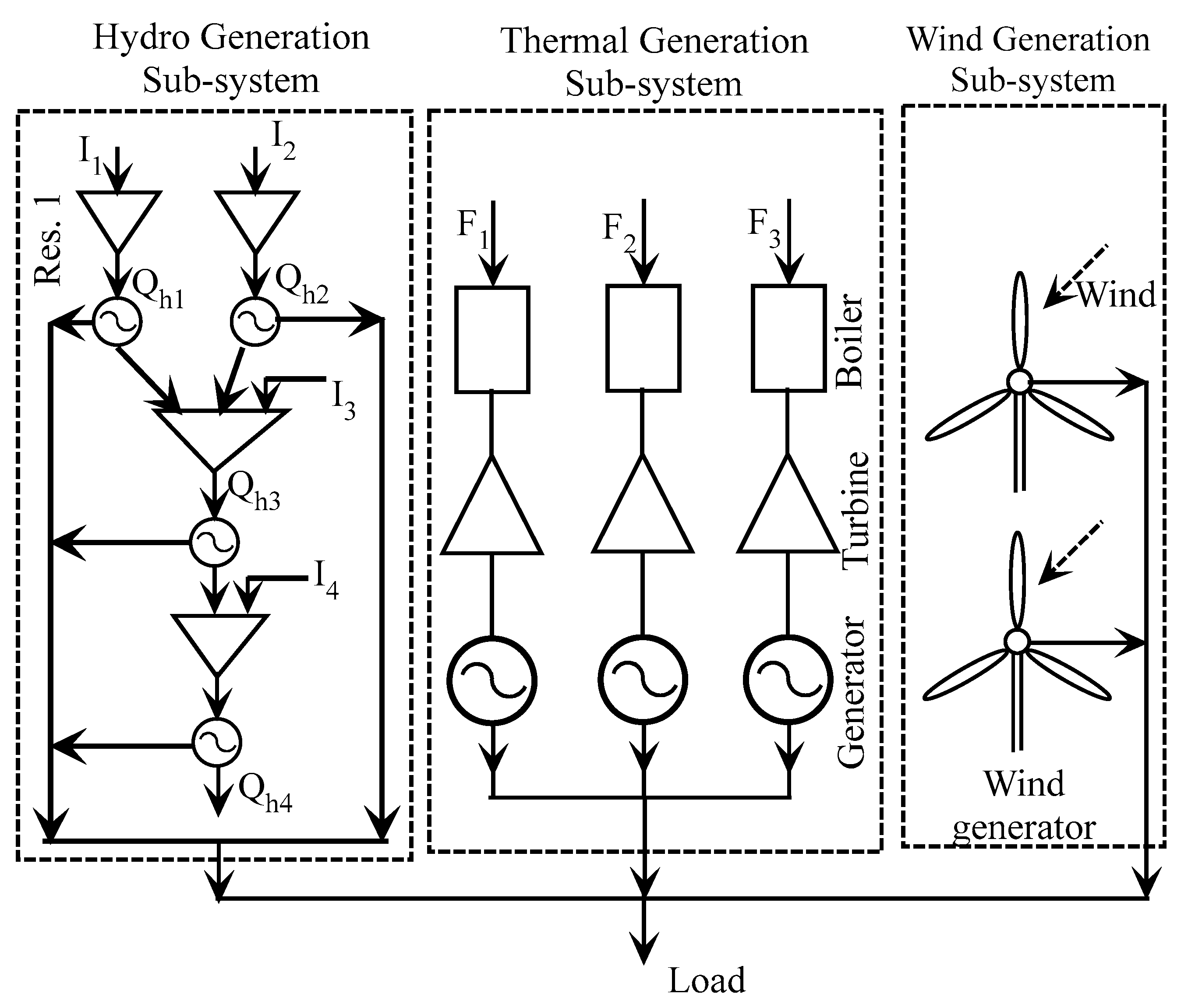
In this work, a test system consisting of a multi-stream cascaded hydro system with four hydro plants, three thermal plants, and two wind plants has been considered for investigating the feasibility and performance of the solution techniques. The schematic diagram of the hydro-thermal-wind test system is shown in Figure 2. The HTWGS considering economic and emission factors has been conducted by implementing the algorithm based on conventional PSO, MPSO, Binary Coded GA, IHS, and JAYA algorithms. The simulations were executed in MATLAB 2015a platform. The program was run 30 times for the test case and the results were analyzed on the basis of the best, average, and worst case with standard deviation. The proposed MPSO shows competency and effectiveness in terms of solution quality and consistency of results.
Thermal system coefficients and constraints are taken from [31]. The hydro system data is taken from [25]. The scheduling period is taken as one-day, which is split into 24 numbers of a 1-h time span. 
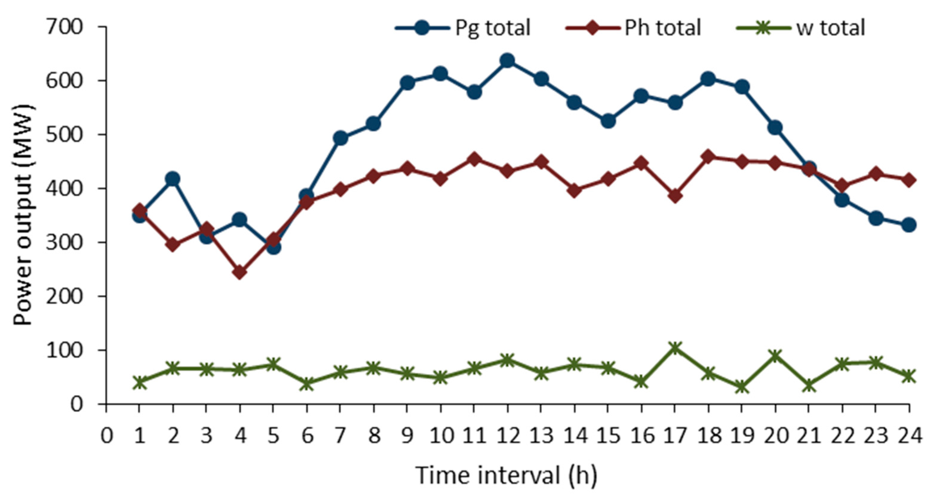
Figure 3 shows the system power demand curve. The wind system parameters are taken from [18,22]. All the necessary data of the hydro-thermal-wind system are shown in Table A1, Table A2, Table A3, Table A4 and Table A5 in Appendix A.
The optimal allocation of demand among the hydro-thermal-wind system and corresponding economic and emission values obtained from the best run are tabulated in the following tables. Table 1 shows the optimal hydro-thermal-wind generation scheduling of the test system accounting for economic and emission factors obtained from the MPSO method. 
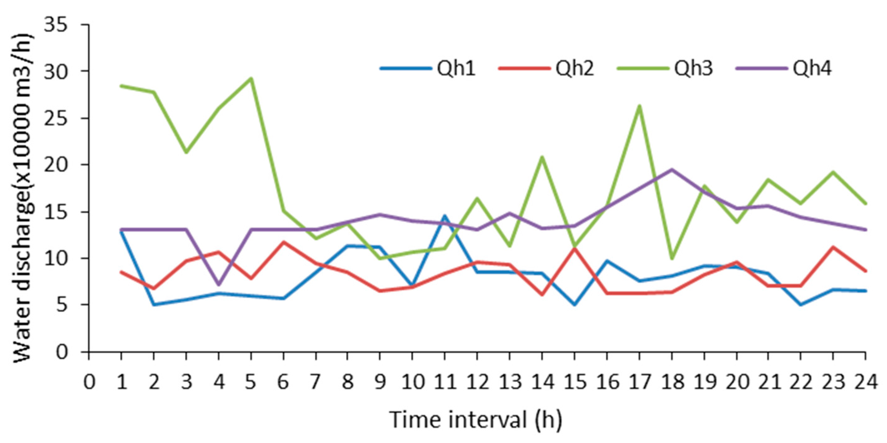
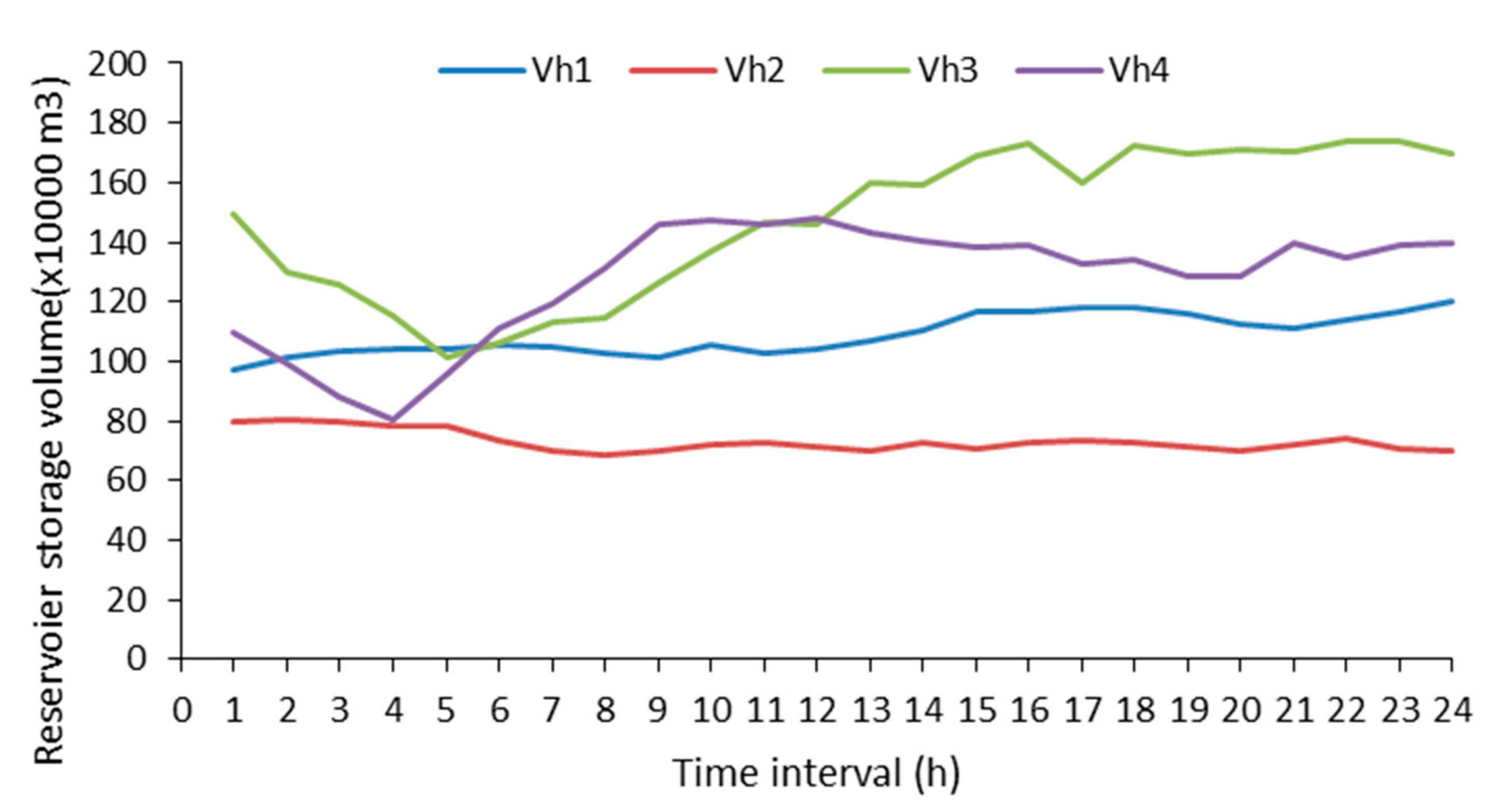
Table 2 presents hourly water discharge and reservoir storage volume values. The storage volume satisfied the end conditions of each reservoir by adjusting the water discharge from each reservoir.
Table 3 shows the total fuel cost, emission, and wind penalty cost of the optimal generation schedule of the test system. Statistical analysis and comparison of performance of the proposed method (MPSO) with other heuristic algorithms (conventional PSO, BCGA, IHS, and JAYA algorithm) in terms of total fuel cost and emission are presented in Table 4. The simulation results obtained using PSO, BCGA, IHS and JAYA methods are shown in Tables S1–S12 in the Supplementary Materials.
The comparison of total fuel cost and emission shown in Table 4 indicates that the MPSO method is capable of providing the optimal generation schedule. Also, the MPSO solution maintains the lower value of standard deviation, representing the consistency in the results compared with conventional PSO, BCGA, IHS, and newly introduced JAYA algorithms. To show a quantitative measure, here the MPSO solution is compared with the next best performing algorithm (conventional PSO). The total fuel cost and emission of pollutants by the MPSO algorithm are $66,083.6629 and 63.4564 lb, respectively, whereas the PSO-based algorithm shows total fuel cost and emission values of $68,646.8010 and 65.7942 lb, respectively. In other words, over the specified time schedule and demands, the proposed MPSO-based method attains an average reduction of 109.7974 $/h in generation cost and 0.0974 lb/h in emission of pollutant compared with the PSO-based algorithm. This quantitative comparison exhibits the efficiency of the MPSO algorithm for providing the optimal generation schedule accounting for economic and emission factors, without being trapped in the local minima.
Figure 4 shows the optimal load allocation among hydro, thermal, and wind plants of the test system over the 24-h time span. The thermal generation shows dominancy from 8.0 h to 20.0 h, because of the increased power demand on the system.
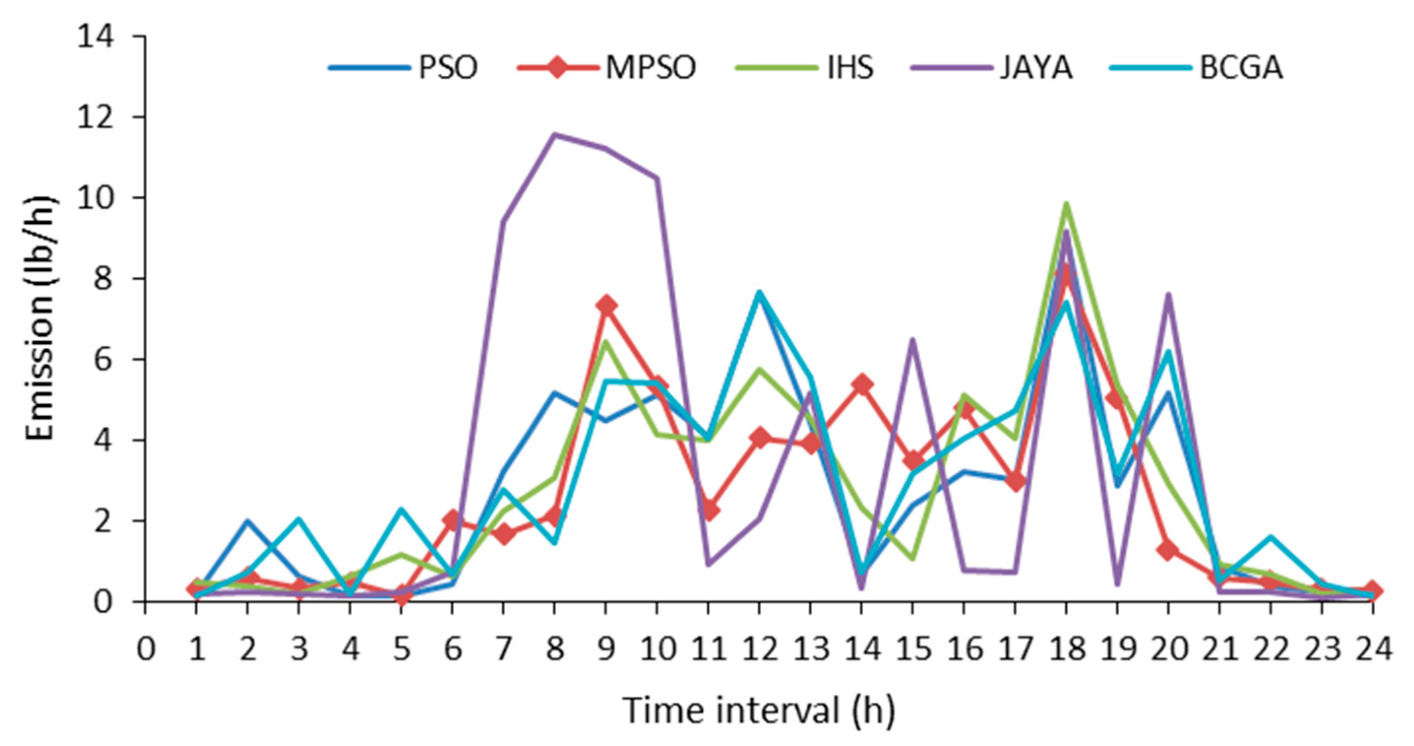
 Figure 5 and Figure 6 show the fuel cost and emission release of thermal plants over the scheduling period obtained by MPSO, PSO, BCGA, IHS, and JAYA algorithms. MPSO maintains a lower fuel cost and emission over the scheduling period.
Figure 7 and Figure 8 show the hourly water discharge from the hydro plant and storage volume of reservoirs, respectively. The convergence characteristics of MPSO, conventional PSO, BCGA, IHS, and JAYA algorithms in terms of total fuel cost are shown in Figure 9. The JAYA method exhibits an almost constant fuel cost in the beginning stage. The MPSO, conventional PSO, BCGA, and IHS methods exhibit a similar curve, but MPSO shows the lowest position.

7. Conclusions

This paper investigated the competency of certain heuristic algorithms representing different heuristic groups, for searching for the optimal generation schedule of an HTW system considering economic and environmental factors. A modified particle swarm optimization (MPSO) method is suggested for the purpose. The proposed modification to the conventional PSO method improved the local search capability of the algorithm and hence delivered a solution with the minimum emission value and lowest overall operating cost. Here, the maximum penalty factor approach was used to transform the multi-objective economic and emission function into a single objective. The computational efficiency of the algorithm is illustrated with a test system consisting of three thermal plants, a multi stream reservoir with four hydro plants, and two wind plants. This algorithm offers a trade-off solution between the generation cost and quantity of emission. The proposed MPSO algorithm, conventional PSO, binary coded GA, IHS, and JAYA algorithm were executed 30 times with the test system and the solutions were compared and analyzed statistically on the basis of the best, average, and worst values, along with the standard deviation. The simulation results showed that MPSO demonstrated a better performance than the other selected algorithms in terms of quality solution and consistency. The salient features of the method are less computational steps and easiness of implementation, which makes the algorithm more suitable for accounting for large-scale hydro-thermal-wind optimal scheduling.

Supplementary Materials

The following are available online at https://www.mdpi.com/1996-1073/11/2/353/s1, Table S1: Optimal generation schedule of the hydro-thermal-wind system obtained using the PSO method, Table S2: Hourly water discharge and reservoir storage volume obtained using the PSO method, Table S3: Fuel cost, rate of pollutant emission, and wind generation penalty cost of the optimal generation schedule-PSO method, Table S4: Optimal generation schedule of the hydro-thermal-wind system obtained using the GA method, Table S5: Hourly water discharge and reservoir storage volume obtained using the GA method, Table S6: Fuel cost, rate of pollutant emission, and wind generation penalty cost of the optimal generation schedule-GA method, Table S7: Optimal generation schedule of the hydro-thermal-wind system obtained using the IHS method, Table S8: Hourly water discharge and reservoir storage volume obtained using the IHS method, Table S9: Fuel cost, rate of pollutant emission, and wind generation penalty cost of the optimal generation schedule-IHS method, Table S10: Optimal generation schedule of the hydro-thermal-wind system obtained using the JAYA method, Table S11: Hourly water discharge and reservoir storage volume obtained using the JAYA method, Table S12: Fuel cost, rate of pollutant emission, and wind generation penalty cost of the optimal generation schedule-JAYA method.

Acknowledgments

The authors gratefully acknowledge the National Institute of Technology Calicut for providing necessary facilities for the conduct of the work. The first author would like to thank the Government of Kerala for providing deputation to pursue doctoral programme under QIP.

Author Contributions

Suresh K. Damodaran completed the coding, execution of programs, compilation of results, and preparation of the paper. T. K. Sunil Kumar was involved in designing and conceptualizing the study.

Conflicts of Interest

The authors declare no conflict of interest.

Appendix A

Table A1. Water inflow time delay between reservoirs.
Plant1234
Ru0021
τd2340
Ru: Number of upstream hydro plants; τd: Time delay to immediate downstream hydro plant.
Table A2. Hydro power generation coefficients.
PlantC1C2C3C4C5C6
1−0.0042−0.420.0300.0910.0−50
2−0.0040−0.300.0151.149.5−70
3−0.0016−0.300.0140.555.5−40
4−0.0030−0.310.0271.4414.0−90
Table A3. Reservoir storage, plant discharge, reservoir end conditions (×104 m3), and hyro plant generation limits.
Plant V h min V h max V h begin V h end Q h min Q h max P h min P h max
1801501001205150500
26012080706150500
310024017017010300500
47016012014013250500
Table A4. Reservoir inflows (×104 m3).
Time PeriodReservoirTime PeriodReservoir
12341234
11088.12.81311840
2988.12.41412930
38941.61511930
479201610820
56830179720
67740188620
78630197710
89720206810
910810217920
1011910228920
1112910239810
12108202410800
Table A5. Wind speed data.
κcυinυrυowr,1 = wr,2ku,1 = ku,2ko,1 = ko,2d1 = d2
2.215515450.815835000

References

  1. Esteban, G.; Juan, A. Short-term Hydrothermal Generation Scheduling Using a Parallelized Stochastic Mixed-integer Linear Programming Algorithm. Energy Procedia 2016, 87, 77–84. [Google Scholar] [CrossRef]
  2. Omid, H.; Behnam, M.; Morteza, N.H.; Somayeh, A. Application of Dynamic Non-Linear Programming Technique to Non-Convex Short-Term Hydrothermal Scheduling Problem. Energies 2017, 10, 1440. [Google Scholar] [CrossRef]
  3. Rafael, N.R.; Edson, L.S.; Erlon, C.F.; Fabricio, Y.K.T. Solving the Short-Term Scheduling Problem of Hydrothermal Systems via Lagrangian Relaxation and Augmented Lagrangian. Math. Probl. Eng. 2012, 2012, 1–18. [Google Scholar] [CrossRef]
  4. Jianxin, T.; Luh, P.B. Hydrothermal scheduling via extended differential dynamic programming and mixed coordination. IEEE Trans. Power Syst. 1995, 10, 2021–2028. [Google Scholar] [CrossRef]
  5. Nazari, H.M.; Mohammadi, I.B.; Gharehpetian, G.B. Short-term scheduling of hydro-based power plants considering application of heuristic algorithms: A comprehensive review. Renew. Sustain. Energy Rev. 2017, 74, 116–129. [Google Scholar] [CrossRef]
  6. Senthil, K.V.; Mohan, M.R. A genetic algorithm solution to the optimal short-term hydrothermal scheduling. Int. J. Electr. Power Energy Syst. 2011, 33, 827–835. [Google Scholar] [CrossRef]
  7. Nazari, H.M.; Mohammadi, B.; Haghrah, A. Optimal short-term generation scheduling of hydrothermal systems by implementation of real-coded genetic algorithm based on improved Mühlenbein mutation. Energy 2017, 128, 77–85. [Google Scholar] [CrossRef]
  8. Glotić, A.; Zamuda, A. Short-term combined economic and emission hydrothermal optimization by surrogate differential evolution. Appl. Energy 2015, 141, 42–56. [Google Scholar] [CrossRef]
  9. Feng, Z.K.; Niu, W.J.; Zhou, J.Z.; Cheng, C.T.; Zhang, Y.C. Scheduling of short-term hydrothermal energy system by parallel multi-objective differential evolution. Appl. Soft Comput. 2017, 61, 58–71. [Google Scholar] [CrossRef]
  10. Mandal, K.K.; Basu, M.; Chakraborty, N. Particle swarm optimization technique based short-term hydrothermal scheduling. Appl. Soft Comput. 2008, 8, 1392–1399. [Google Scholar] [CrossRef]
  11. Nitin, N.; Dhillonb, J.S.; Kotharic, D.P. Scheduling short-term hydrothermal generation using predator prey optimization technique. Appl. Soft Comput. 2014, 21, 298–308. [Google Scholar] [CrossRef]
  12. Jadhav, H.; Roy, R. Gbest guided artificial bee colony algorithm for environmental/economic dispatch considering wind power. Expert Syst. Appl. 2013, 40, 6385–6399. [Google Scholar] [CrossRef]
  13. Shanhe, J.; Zhicheng, J.; Yan, W. A novel gravitational acceleration enhanced particle swarm optimization algorithm for wind–thermal economic emission dispatch problem considering wind power availability. Int. J. Electr. Power Energy Syst. 2015, 73, 1035–1050. [Google Scholar] [CrossRef]
  14. Geem, Z.W.; Kim, J.H.; Loganathan, G.V. A new heuristic optimization algorithm: Harmony search. Simulation 2001, 76, 60–68. [Google Scholar] [CrossRef]
  15. Ren, P.; Li, N. Short-Term Hydrothermal Scheduling Based on Harmony Search Algorithm. Adv. Mater. Res. 2014, 1044–1045, 1507–1510. [Google Scholar] [CrossRef]
  16. Warid, W.; Hashim, H.; Norman, M.; Noor, I.A.-W. Optimal Power Flow Using the Jaya Algorithm. Energies 2016, 9, 678. [Google Scholar] [CrossRef]
  17. Hetzer, J.; Yu, D.C.; Bhattarai, K. An economic dispatch model incorporating wind power. IEEE Trans. Energy Convers. 2008, 23, 603–611. [Google Scholar] [CrossRef]
  18. Liu, X.; Xu, W. Minimum emission dispatch constrained by stochastic wind power availability and cost. IEEE Trans. Power Syst. 2010, 25, 1705–1713. [Google Scholar] [CrossRef]
  19. Xian, L. Economic Load Dispatch Constrained by Wind Power Availability: A Wait-and-See Approach. IEEE Trans. Smart Grid 2010, 1, 347–355. [Google Scholar] [CrossRef]
  20. Karami, M.; Shayanfar, H.A.; Aghaei, J.; Ahmadi, A. Scenario-based security-constrained hydrothermal coordination with volatile wind power generation. Renew. Sustain. Energy Rev. 2013, 28, 726–737. [Google Scholar] [CrossRef]
  21. Yuan, X.; Tian, H.; Yuan, Y.; Huang, Y.; Ikram, R.M. An extended NSGA-III for solution multi-objective hydro-thermal-wind scheduling considering wind power cost. Energy Convers. Manag. 2015, 96, 568–578. [Google Scholar] [CrossRef]
  22. Jianzhong, Z.; Peng, L.; Yuanzheng, L.; Chao, W.; Liu, Y.; Li, M. Short-term hydro-thermal-wind complementary scheduling considering uncertainty of wind power using an enhanced multi-objective bee colony optimization algorithm. Energy Convers. Manag. 2016, 123, 116–129. [Google Scholar] [CrossRef]
  23. Chen, Y.; Wei, W.; Liu, F.; Mei, S. Distributionally robust hydro-thermal-wind economic dispatch. Appl. Energy 2016, 173, 511–519. [Google Scholar] [CrossRef]
  24. De Moraes, R.A.; Fernandes, T.S.P.; Arantes, A.G.B.; Unsihuay-Vila, C. Short-term scheduling of integrated power and spinning reserve of a wind-hydrothermal generation system with ac network security constraints. J. Control Atom. Electr. Syst. 2018, 29, 1–14. [Google Scholar] [CrossRef]
  25. Orero, S.O.; Irving, M.R. A Genetic Algorithm Modelling Framework and Solution Technique for Short Term Optimal Hydrothermal Scheduling. IEEE Trans. Power Syst. 1998, 13, 501–518. [Google Scholar] [CrossRef]
  26. Güvenç, U.; Sönmez, Y.; Duman, S.; Yörükeren, N. Combined economic and emission dispatch solution using gravitational search algorithm. Sci. Iran 2012, 19, 1754–1762. [Google Scholar] [CrossRef]
  27. Kothari, D.P.; Dhillon, D.H. Power System Optimization, 2nd ed.; PHI Learning Pvt. Ltd.: New Delhi, India, 2011; pp. 249–324. [Google Scholar]
  28. Yuan, X.; Wang, L.; Zhang, Y.; Yuan, Y. A hybrid differential evolution method for dynamic economic dispatch with valve-point effects. Expert Syst. Appl. 2009, 36, 4042–4048. [Google Scholar] [CrossRef]
  29. Mahdavi, M.; Fesanghary, M.; Damangir, E. An improved harmony search algorithm for solving optimization problems. Appl. Math. Comput. 2007, 188, 1567–1579. [Google Scholar] [CrossRef]
  30. Venkata Rao, R. Jaya: A simple and new optimization algorithm for solving constrained and unconstrained optimization problems. Int. J. Ind. Eng. Comput. 2016, 7, 19–34. [Google Scholar] [CrossRef]
  31. Basu, M. An interactive fuzzy satisfying method based on evolutionary programming technique for multiobjective short-term hydrothermal scheduling. Elect. Power Syst. Res. 2004, 69, 277–285. [Google Scholar] [CrossRef]
Figure 1. Flow chart of the proposed MPSO method.
Energies 11 00353 g001
Figure 2. Schematic diagram of the hydro-thermal-wind test system.
Energies 11 00353 g002
Figure 3. Load curve.
Energies 11 00353 g003
Figure 4. Optimal power generation schedules from the MPSO algorithm over 24 h time span.
Energies 11 00353 g004
Figure 5. Fuel cost curve obtained from the MPSO, PSO, BCGA, IHS, and JAYA algorithms over the scheduling time.
Energies 11 00353 g005
Figure 6. Emission curves obtained from MPSO, PSO, BCGA, IHS, and JAYA algorithms over the scheduling time.
Energies 11 00353 g006
Figure 7. Hydro plant discharge curves.
Energies 11 00353 g007
Figure 8. Hydro plant reservoir storage volume curves.
Energies 11 00353 g008
Figure 9. Convergence characteristics of MPSO, PSO, BCGA, IHS, and JAYA algorithms in terms of total fuel cost.
Energies 11 00353 g009
Table 1. Optimal generation schedule of the hydro-thermal-wind system obtained using the MPSO method.
Time PeriodLoad (MW)Hydro Generation (MW)Thermal GenerationWind Generation
Ph1Ph2Ph3Ph4Pg1 (MW)Pg2 (MW)Pg3 (MW)w1 (MW)w2 (MW)
175094.344664.60980200.093797.0717171.715581.141113.957827.0658
278053.216854.78130187.7553111.0668197.9873108.959334.561531.6717
370058.397771.374921.6249173.733385.8489173.79025040.316424.9138
465063.559574.63220106.128775.7075190.903675.682223.024540.3618
567061.514760.41670184.0039125.9647114.5835041.749831.7672
680060.071875.479437.5928201.27393.3212244.23755010.604827.4194
795080.071563.205743.6685210.5434175235.374483.319725.433433.3833
8101092.326857.372443.0301230.708152.4463244.8935122.423533.050233.7493
9109091.635146.378346.5969252.941153.8851285.6351156.712135.182421.0341
10108069.795750.512150.3702247.5302165.8896275.2491171.953430.182718.5171
11110099.665859.318853.1227243.5127170.4439246.0919161.454231.504634.8855
12115079.610664.582449.1105238.7893175265.7111195.734236.680744.7814
13111080.469662.187556.265250.6784174.1035264.8422164.285533.737723.4305
14103080.569745.092538.0304233.5562170.515275.617113.67238.342334.6049
15101054.811970.526957.8224234.0562173.1186261.225490.530535.932331.9758
16106089.514146.346457.8832252.4703174.9847271.7981125.096131.208410.6987
17105076.200846.54972.6721261.2708174.9083255.7756128.480163.145640.997
18112080.23546.819756.4534275.2267175288.7387140.283926.389930.8527
19107086.293758.113752.4138253.7575175273.5513139.26438.698322.9074
20105084.479663.807159.096240.8272175225.3728111.674854.370835.3717
2191080.545150.861850.9588253.8385172.3393191.143275.04318.79416.4763
2286055.362652.402357.7269240.1722134.3991188.044856.672125.70249.5181
2385069.21371.340549.0087238.005186.1625168.414890.894933.486143.4744
2480068.382159.211356.7243231.5578.7156166.838786.973612.05239.5524
Table 2. Hourly water discharge and reservoir storage volume obtained using the MPSO method.
Time PeriodWater Discharge (×104 m3/h)Reservoir Storage Volume (×104 m3)
Qh1Qh2Qh3Qh4Vh1Vh2Vh3Vh4
112.81998.5128.40741397.180179.49149.6926109.8
25.05516.780127.757313101.12580.7099130.135299.2
35.60219.748721.422613103.522979.9612125.532587.8
46.215510.713926.06317.1202104.307478.2473115.034680.6798
55.95947.908129.313613104.34878.3392101.103296.0872
65.754711.775915.007413105.593373.5633106.0601110.8445
78.57389.454112.18413105.019670.1092113.5494119.2671
811.30088.534913.792613.8042102.718868.5743114.8546131.526
911.23966.53821014.669101.479270.036126.2042146.1706
107.00326.962310.683413.9647105.47672.0738137.1593147.2132
1114.58728.360611.034513.6862102.888872.7132146.8993145.711
128.5279.587616.449713104.361871.1255145.9911147.8044
138.56079.287111.330214.756106.80169.8384160.2103143.0484
148.43566.082820.795613.1501110.365472.7557159.3023140.5818
15511.00511.263613.4466116.365470.7506169.1871138.1697
169.74866.293415.613315.424116.616872.4572173.2965139.1953
177.57656.251826.353817.4795118.040473.2054160.0255133.0461
188.16216.3221019.5147117.878372.8834172.7791134.3269
199.20138.281717.806417.1321115.67771.6017169.8426128.4584
208.99849.593613.903415.3456112.678670.0081171.353128.7261
218.39937.026718.35615.5498111.279371.9814170.5203139.5301
225.07917.067715.816114.4662114.200273.9136173.9843135.0639
236.674711.226119.192313.7738116.525570.6875173.7849139.0966
246.52558.687515.89071312070170140
Table 3. Fuel cost, rate of pollutant emission, and wind generation penalty cost of the optimal generation schedule-MPSO method.
Time PeriodFuel Cost ($/h)Emission (lb/h)Wind Generation Penalty Cost ($/MWh)
Underestimation, Cu,iOverestimation, Co,iTotal Penalty Cost ($/MWh)
11611.8840.32368836.25425046.142913,882.3971
22209.56460.59944337.219812,622.756616,959.9764
31304.47730.32654749.063913,058.523417,807.5873
41654.35480.47355092.851412,550.88217,643.7334
51004.65940.16283468.762616,177.837419,646.6
61959.85352.00639556.48924730.250214,286.7394
72439.47431.67615522.84539957.041115,479.8865
83005.14772.14024247.544212,829.030817,076.575
94086.22787.32976102.08519540.161115,642.2462
104336.28125.34887335.85886940.099514,275.9583
113810.89992.28334318.472512,699.246617,017.7192
124821.58914.06222506.830920,009.380722,516.2116
134078.53913.92185838.56799529.733515,368.3015
143248.4745.37333438.999415,590.394919,029.3943
152789.24183.47514110.129113,353.519817,463.6489
163395.43024.79828926.32876096.013415,022.3421
173280.18532.98391187.668135,464.472336,652.1403
183853.99378.11355727.56569242.671514,970.2372
193666.54575.071210,827.36973198.178214,025.5479
202706.87831.30522055.313625,747.121227,802.4348
211926.31720.60379842.24483251.189113,093.434
221610.36940.49593810.94518,735.337822,546.2828
231679.39870.29833051.193417,836.440520,887.6339
241603.87590.28387505.41819991.129217,496.5473
Total66,083.662963.4563132,396.0213304,197.5537436,593.5754
Table 4. Statistical analysis of the heuristic algorithms in terms of total fuel cost and emission.
MethodFuel Cost ($/h)Emission (lb/h)
BestAverageWorstStd. Dev.BestAverageWorstStd. Dev.
MPSO66,083.662966,086.746266,089.37231.658663.456464.199864.97460.4732
PSO68,646.801068,649.494868,652.15551.663465.794266.710767.47180.5176
GA71,016.972471,021.026771,025.93142.897370.745771.999873.31020.7616
IHS71,300.971671,305.704371,309.30332.594966.463067.692968.89290.7339
JAYA85,394.027185,404.162985,414.34175.638379.035180.599182.32400.9574

