Application of H∞ Robust Control on a Scaled Offshore Oil and Gas De-Oiling Facility


Abstract
:1. Introduction
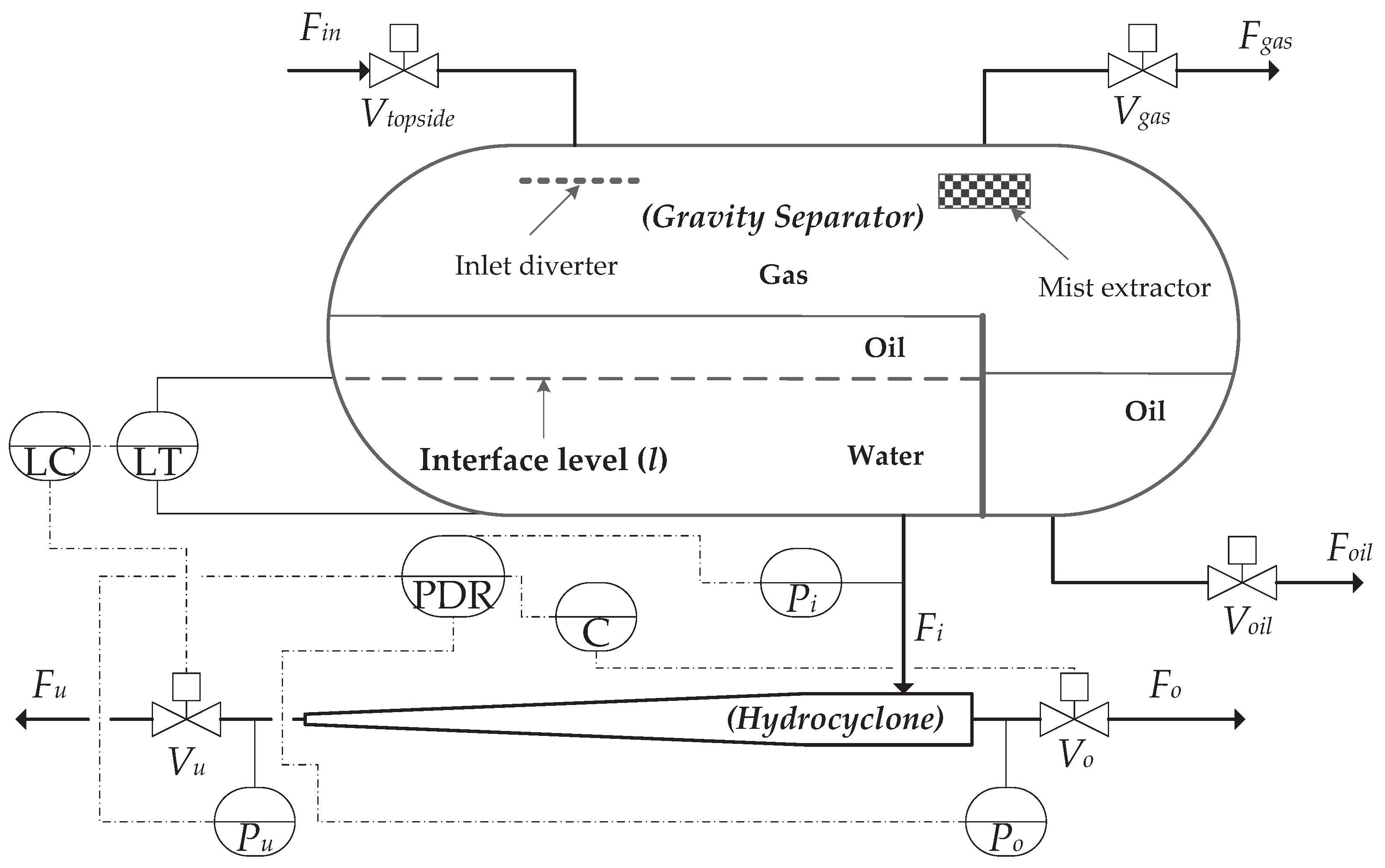
2. De-Oiling Process Model
2.1. Model Development
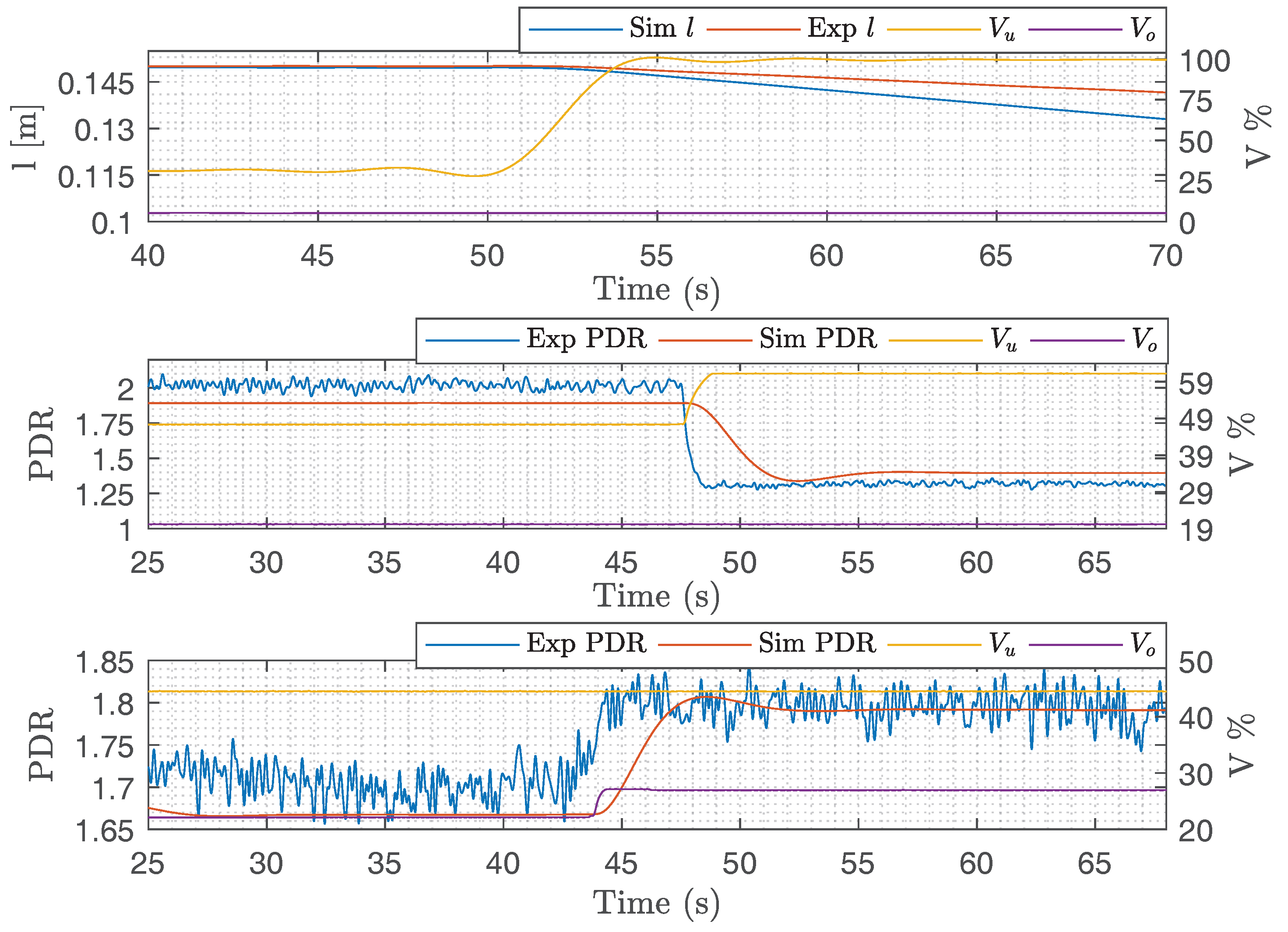
2.2. Model Validation
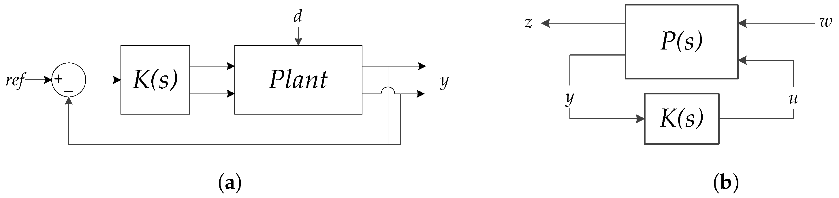
3. Synthesis of the Robust Control Solution
3.1. Numerical Solvability
3.1.1. Assumption 1
3.1.2. Assumption 2
3.1.3. Assumption 3
3.1.4. Assumption 4
3.2. H Controller Synthesis
- H with ;
- J with ; and
- .
3.3. The Designed H Controller
4. Benchmark PID Control Solution
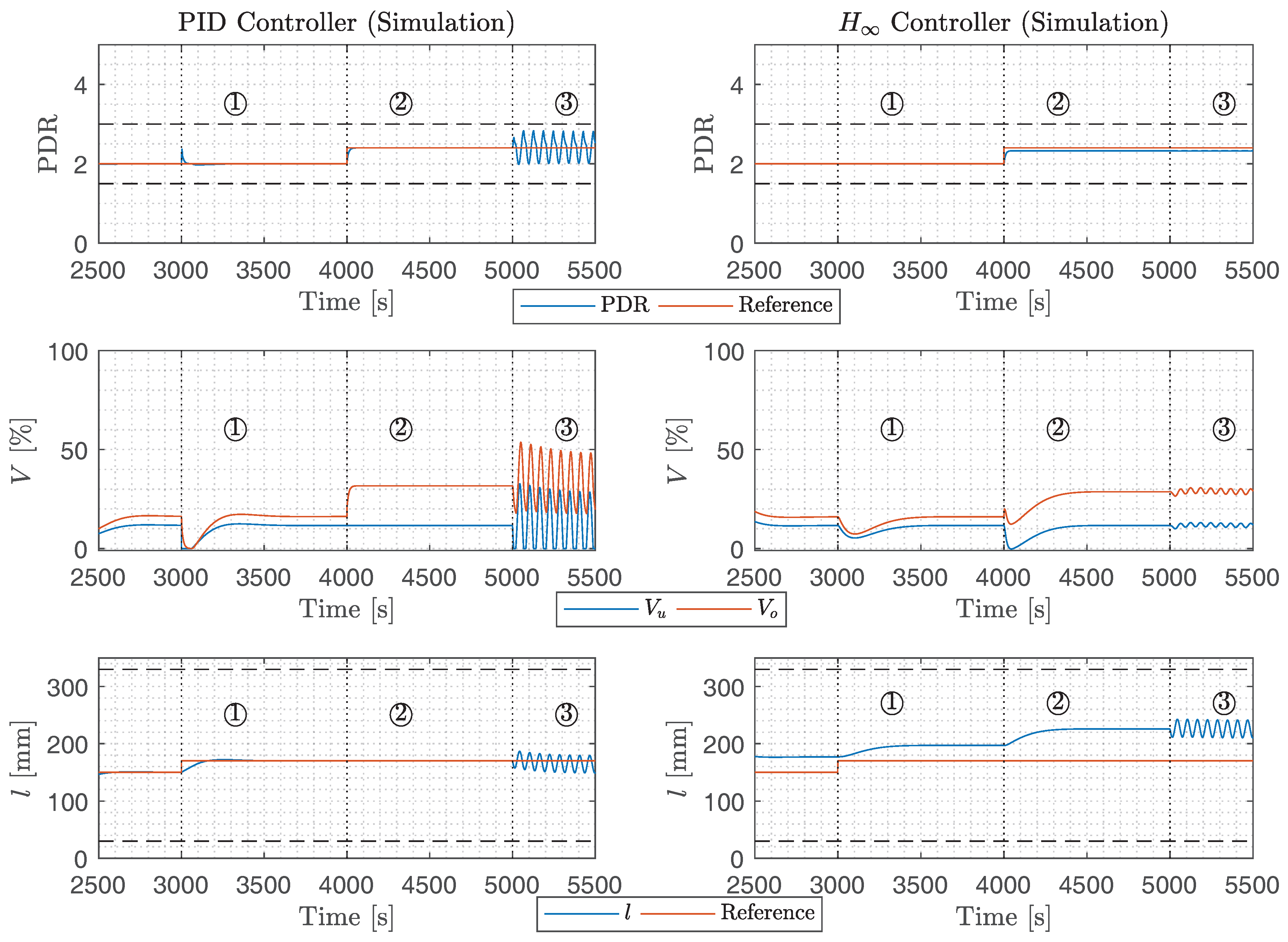
5. Performance Analysis via Simulation
5.1. Description of the Testing Scenarios
5.1.1. Scenario ①
5.1.2. Scenario ②
5.1.3. Scenario ③
5.2. Simulation Results
6. Scaled Pilot Plant Implementation
6.1. Scaled Pilot Plant Experiment Description
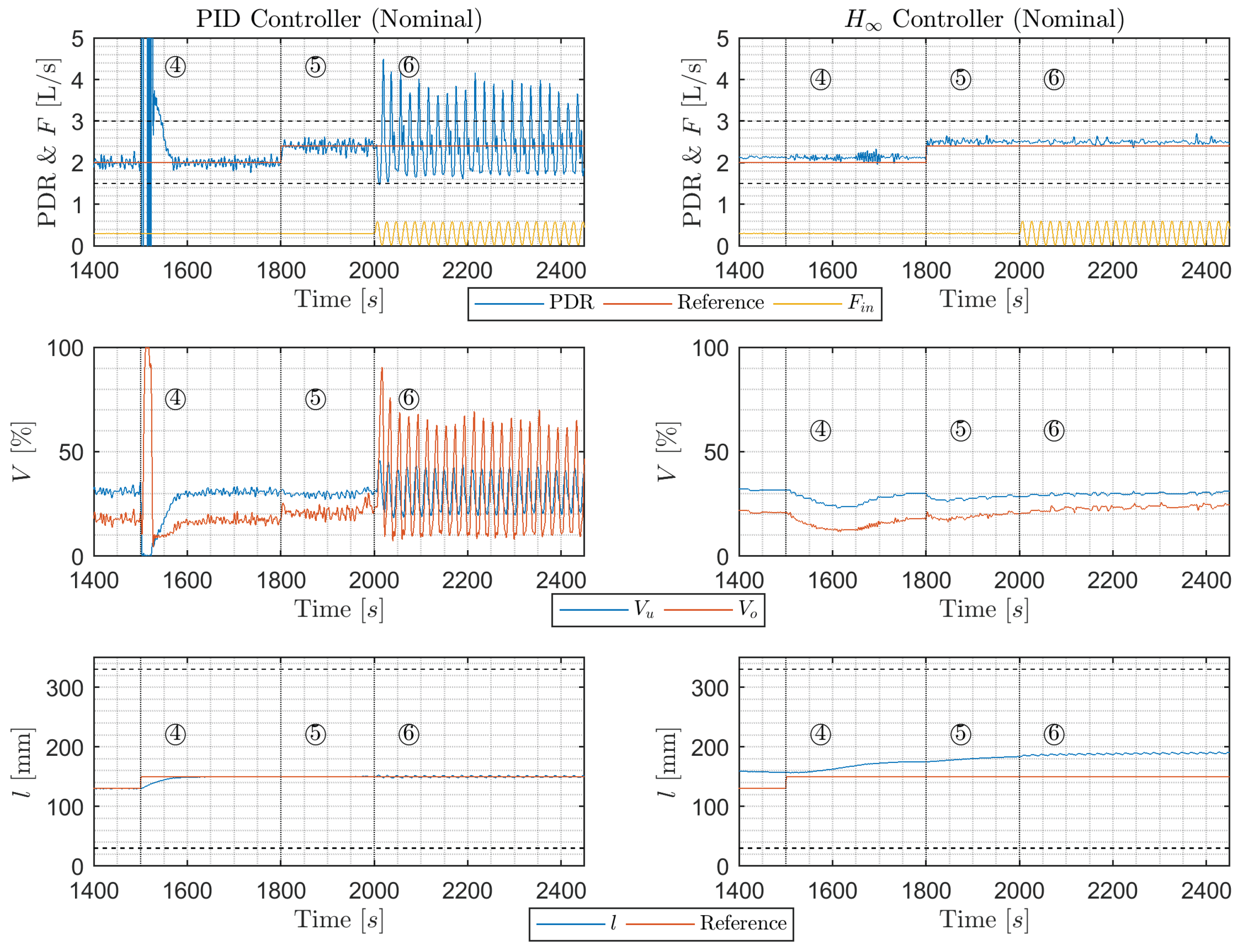
6.2. Results of Experiments Performed on the Scaled Pilot Plant
6.2.1. Experiment Results for Scenario ④
6.2.2. Experiment Results for Scenario ⑤
6.2.3. Experiment Results for Scenario ⑥
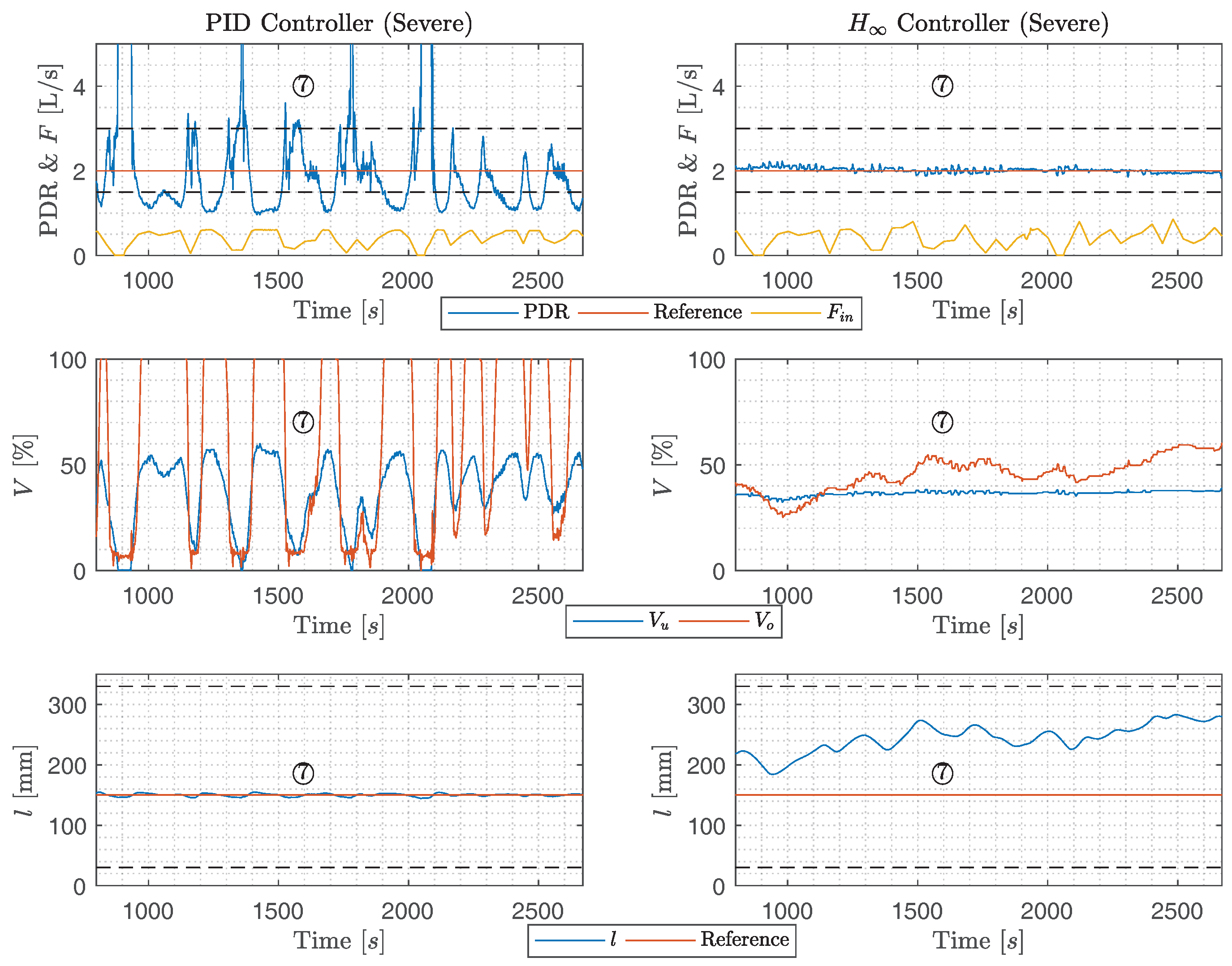
6.2.4. Experiment Results for Scenario ⑦
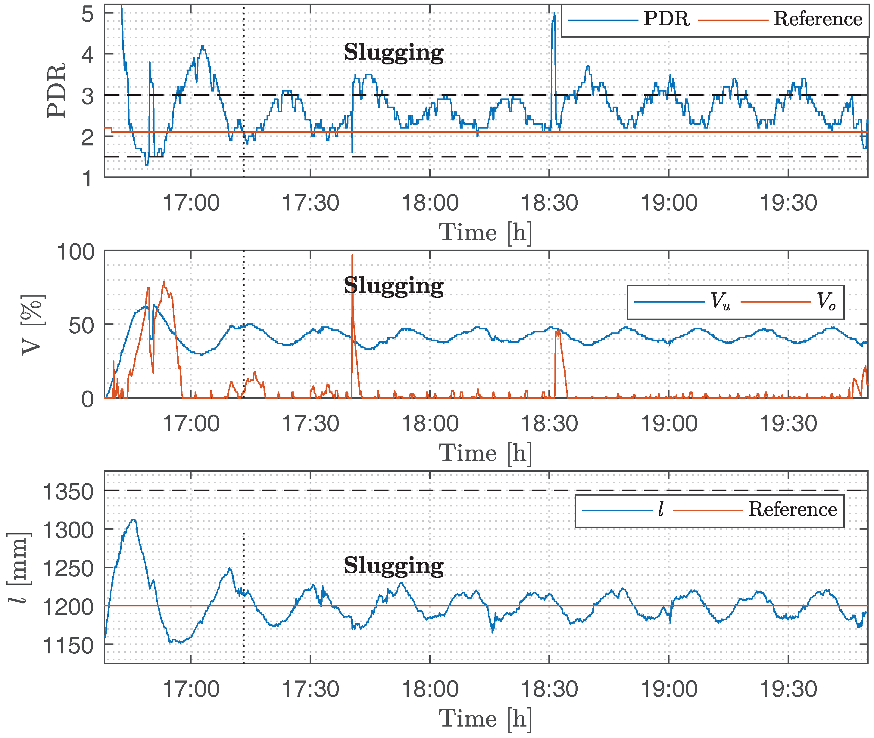
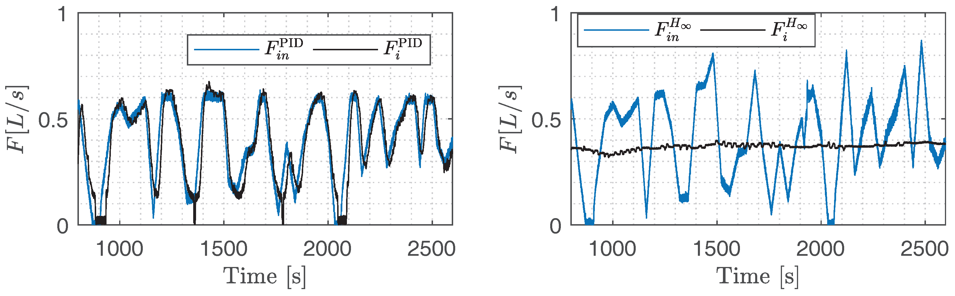
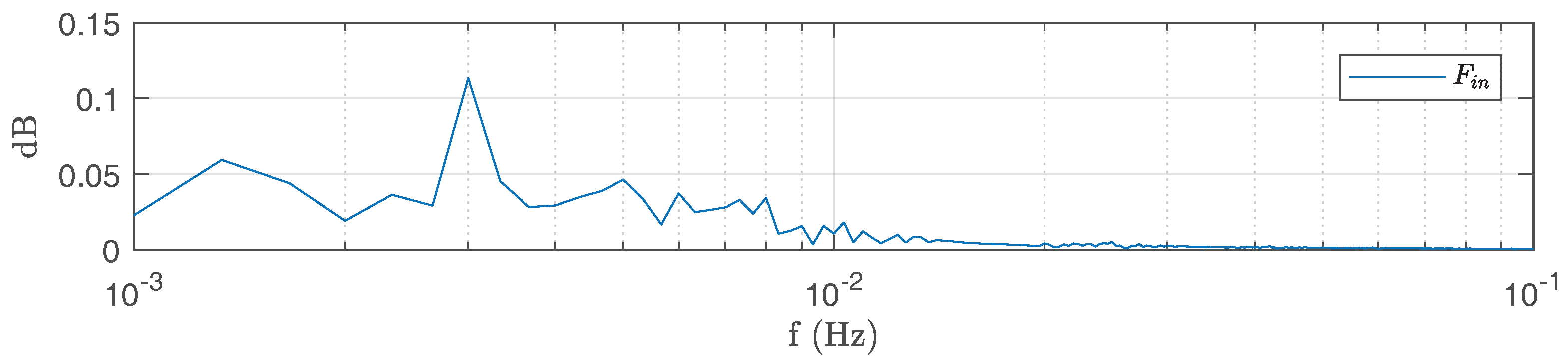
6.3. Transmission of Fluctuations in
7. Discussion
7.1. Simulation Results
7.2. Experimental Results
8. Conclusions
Acknowledgments
Author Contributions
Conflicts of Interest
References
- Bamberg, J. British Petroleum and Global Oil 1950–1975: The Challenge of Nationalism; British Petroleum Series; Cambridge University Press: Cambridge, UK, 2000. [Google Scholar]
- Ekins, P.; Vanner, R.; Firebrace, J. Zero emissions of oil in water from offshore oil and gas installations: Economic and environmental implications. J. Clean. Prod. 2007, 15, 1302–1315. [Google Scholar] [CrossRef]
- Stephenson, M. A survey of produced water studies. In Produced Water; Springer: Berlin/Heidelberg, Germany, 1992; pp. 1–11. [Google Scholar]
- Bailey, B.; Crabtree, M.; Tyrie, J.; Elphick, J.; Kuchuk, F.; Romano, C.; Roodhart, L. Water control. Oilfield Rev. 2000, 12, 30–51. [Google Scholar]
- Veil, J.A.; Puder, M.G.; Elcock, D.; Redweik, R.J., Jr. A White Paper Describing Produced Water From Production of Crude Oil, Natural Gas, and Coal Bed Methane; Technical Report; Argonne National Laboratory: Lemont, IL, USA, 2004; Volume 63.
- Danish Production of Oil, Gas and Water (Danish Energy Agency). Available online: https://ens.dk/en/our-services/oil-and-gas-related-data/monthly-and-yearly-production (accessed on 1 November 2016).
- Miljoestyrelsen. Status for Den Danske Offshorehandlingsplan Til Udgangen Af 2009. Miljoestyrelsen. Available online: http://www.ft.dk/samling/20101/almdel/MPU/bilag/66/903508.pdf (accessed on 1 October 2017).
- Miljoestyrelsen. Afsluttende rapport for de danske offshorehandlingsplaner 2005–2010. Miljoestyrelsen. Available online: http://mst.dk/media/91455/Bilag%203%20Statusrapport%20OHP%202013%20rev%20(2).pdf (accessed on 1 October 2017).
- Methodology for the Sampling and Analysis of Produced Water and Other Hydrocarbon Discharges. Available online: https://www.gov.uk/guidance/oil-and-gas-offshore-environmental-legislation (accessed on 3 November 2016).
- OSPAR Commission, About OSPAR. Available online: https://www.ospar.org/about (accessed on 10 January 2018).
- Miljoestyrelsen. Generel Tilladelse for MæRsk Olie Og Gas A/S (MæRsk Olie) Til Anvendelse, Udledning Og Anden Bortskaffelse Af Stoffer Og Materialer, Herunder Olie Og Kemikalier I Produktions-Og Injektionsvand Fra Produktionsenhederne Halfdan, Dan, Tyra Og Gorm for Perioden 1. Januar 2017-31. December 2018. Miljoestyrelsen. Available online: http://mst.dk/media/92144/20161221-ann-generel-udledningstilladelse-for-maersk-olie-og-gas-2017-18.pdf (accessed on 19 October 2017).
- Monnery, W.D.; Svrcek, W.Y. Successfully Specify 3-Phase Separators. Chem. Eng. Prog. 1994, 90, 29–40. [Google Scholar]
- Sayda, A.F.; Taylor, J.H. Modeling and control of three-phase gravilty separators in oil production facilities. In Proceedings of the American Control Conference, New York, NY, USA, 9–13 July 2007; pp. 4847–4853. [Google Scholar]
- Thew, M. Hydrocyclone redesign for liquid-liquid separation. Chem. Eng. (London) 1986, 427, 17–23. [Google Scholar]
- Husveg, T.; Rambeau, O.; Drengstig, T.; Bilstad, T. Performance of a deoiling hydrocyclone during variable flow rates. Miner. Eng. 2007, 20, 368–379. [Google Scholar] [CrossRef]
- Ditria, J.; Hoyack, M. The separation of solids and liquids with hydrocyclone-based technology for water treatment and crude processing. In SPE Asia Pacific Oil and Gas Conference; Society of Petroleum Engineers: London, UK, 1994. [Google Scholar]
- VORTOIL Deoiling Hydrocyclones. Available online: http://www.slb.com/~/media/Files/processing-separation/product-sheets/vortoil-ps.pdf (accessed on 20 October 2017).
- Husveg, T.; Johansen, O.; Bilstad, T. Operational Control of Hydrocyclones during Variable Produced Water Flow Rates—Frøy Case Study. SPE Prod. Oper. 2007, 22, 294–300. [Google Scholar] [CrossRef]
- Husveg, T. Operational Control of Deoiling Hydrocyclones and Cyclones for Petroleum Flow Control. Ph.D. Thesis, University of Stavanger, Stavanger, Norway, 2007. [Google Scholar]
- Durdevic, P.; Raju, C.S.; Bram, M.V.; Hansen, D.S.; Yang, Z. Dynamic Oil-in-Water Concentration Acquisition on a Pilot-Scaled Offshore Water-Oil Separation Facility. Sensors 2017, 17, 124. [Google Scholar] [CrossRef] [PubMed]
- Di Meglio, F.; Kaasa, G.O.; Petit, N.; Alstad, V. Model-based control of slugging: Advances and challenges. IFAC Proc. Vol. (IFAC PapersOnline) 2012, 1, 109–115. [Google Scholar] [CrossRef]
- Sausen, A.; de Campos, M.; Sausen, P. The Slug Flow Problem in Oil Industry and Pi Level Control; InTech Open Access Publisher: London, UK, 2012. [Google Scholar]
- Pedersen, S.; Durdevic, P.; Yang, Z. Review of Slug Detection, Modeling and Control Techniques for Offshore Oil & Gas Production Processes. IFAC PapersOnLine 2015, 48, 89–96. [Google Scholar]
- Durdevic, P.; Pedersen, S.; Yang, Z. Challenges in Modelling and Control of Offshore De-oiling Hydrocyclone Systems. J. Phys. Conf. Ser. 2017, 783, 012048. [Google Scholar] [CrossRef]
- Meldrum, N. Hydrocyclones: A Solution to Produced-Water Treatment. In SPE Production Engineering; University of Michigan: Ann Arbor, MI, USA, 1988; Volume 3, pp. 669–676. [Google Scholar]
- Thew, M.; Smyth, I. Development and performance of oil-water hydrocyclone separators: A review. In Proceedings of the IMM Conference on Innovation in Physical Separation Technologies, Southampton, UK, 1 January 1998. [Google Scholar]
- Durdevic, P.; Pedersen, S.; Yang, Z. Operational Performance of Offshore De-oiling Hydrocyclone Systems. In Proceedings of the 43rd Annual Conference of the IEEE Industrial Electronics Society (IECON), Beijing, China, 29 October–1 November 2017; Volume 43, pp. 6905–6910. [Google Scholar]
- Durdevic, P. Real-Time Monitoring and Robust Control of Offshore De-oiling Processes. Ph.D. Thesis, Aalborg University, Aalborg, Denmark, 2017. [Google Scholar]
- Mokhatab, S.; Poe, W.; Speight, J. Handbook of Natural Gas Transmission and Processing; Chemical, Petrochemical & Process, Gulf Professional Pub.: London, UK, 2006. [Google Scholar]
- Judd, S.; Qiblawey, H.; Al-Marri, M.; Clarkin, C.; Watson, S.; Ahmed, A.; Bach, S. The size and performance of offshore produced water oil-removal technologies for reinjection. Sep. Purif. Technol. 2014, 134, 241–246. [Google Scholar] [CrossRef]
- Yang, Z.; Juhl, M.; Lø hndorf, B. On the innovation of level control of an offshore three-phase separator. In Proceedings of the IEEE International Conference on Mechatronics and Automation, ICMA 2010, Xi’an, China, 4–7 August 2010; pp. 1348–1353. [Google Scholar]
- Rietema, K.; Maatschappij, S.I.R. Performance and design of hydrocyclones—III: Separating power of the hydrocyclone. Chem. Eng. Sci. 1961, 15, 310–319. [Google Scholar] [CrossRef]
- Wolbert, D.; Ma, B.-F.; Aurelle, Y.; Seureau, J. Efficiency estimation of liquid-liquid Hydrocyclones using trajectory analysis. AIChE J. 1995, 41, 1395–1402. [Google Scholar] [CrossRef]
- Thew, M.T. Cyclones for oil/water separation. In Encyclopaedia of Separation Science, 4th ed.; Academic Press: Cambridge, MA, USA, 2000; pp. 1480–1490. [Google Scholar]
- Kharoua, N.; Khezzar, L.; Nemouchi, Z. Hydrocyclones for de-oiling applications—A review. Pet. Sci. Technol. 2010, 28, 738–755. [Google Scholar] [CrossRef]
- Thew, M.; Silk, S.; Colman, D. Determination and use of residence time distributions for two hydrocyclones. In Proceedings of the International conference on Hydrocyclones, Cambridge, UK, 1–3 October 1980; pp. 225–248. [Google Scholar]
- Young, G.; Wakley, W.; Taggart, D.; Andrews, S.; Worrell, J. Oil-water separation using hydrocyclones: An experimental search for optimum dimensions. J. Petrol. Sci. Eng. 1994, 11, 37–50. [Google Scholar] [CrossRef]
- Bram, M.V.; Hassan, A.A.; Hansen, D.S.; Durdevic, P.; Pedersen, S.; Yang, Z. Experimental modeling of a deoiling hydrocyclone system. In Proceedings of the 20th International Conference on Methods and Models in Automation and Robotics, Miedzyzdroje, Poland, 24–27 August 2015; pp. 1080–1085. [Google Scholar]
- Durdevic, P.; Pedersen, S.; Bram, M.; Hansen, D.; Hassan, A.; Yang, Z. Control Oriented Modeling of a De-oiling Hydrocyclone. IFAC PapersOnLine 2015, 48, 291–296. [Google Scholar] [CrossRef]
- Zhou, K.; Doyle, J.C.; Glover, K. Robust and Optimal Control; Prentice Hall: Upper Saddle River, NJ, USA, 1996; Volume 40. [Google Scholar]
- Zhou, K.; Doyle, J.C. Essentials of Robust Control; Prentice Hall: Upper Saddle River, NJ, USA, 1998; Volume 104. [Google Scholar]
- Glover, K.; Doyle, J.C. State-space formulae for all stabilizing controllers that satisfy an H∞-norm bound and relations to relations to risk sensitivity. Syst. Control Lett. 1988, 11, 167–172. [Google Scholar] [CrossRef]
- Kalman, R.E. Mathematical description of linear dynamical systems. J. Soc. Ind. Appl. Math. Ser. A Control 1963, 1, 152–192. [Google Scholar] [CrossRef]
- Gu, D.; Petkov, P.; Konstantinov, M.M. Robust Control Design With MATLAB, 2nd ed.; Springer Science & Business Media: New York, NY, USA, 2005. [Google Scholar]
- Skogestad, S.; Postlethwaite, I. Multivariable Feedback Control: Analysis and Design; Wiley: New York, NY, USA, 2007; Volume 2. [Google Scholar]
- Balas, G.; Chiang, R.; Packard, A.; Safonov, M. Robust control toolbox. In For Use with Matlab. User’s Guide, Version 3; The Mathworks, Inc.: Natick, MA, USA, 2005; Volume 3. [Google Scholar]
- Yang, Z.; Pedersen, S.; Durdevic, P. Cleaning the produced water in offshore oil production by using plant-wide optimal control strategy. In Proceedings of the 2014 Oceans—St. John’s, St. John’s, NL, Canada, 14–19 September 2014; pp. 1–10. [Google Scholar]
- Yang, Z.; Pedersen, S.; Durdevic, P.L.; Mai, C.; Hansen, L.; Jepsen, K.L.; Aillos, A.; Andreasen, A. Plant-wide Control Strategy for Improving Produced Water Treatment. In Proceedings of the 2016 International Field Exploration and Development Conference (IFEDC), Beijing, China, 11–12 August 2016. [Google Scholar]


| A | B | C |
|---|---|---|
| Platform | l | PDR | ||
|---|---|---|---|---|
| Offshore | ||||
| Pilot Plant | ||||
| Simulation |
| Scenario Name | Value & Time | Description |
|---|---|---|
| ① | l = [150 mm–170 mm] @ t = 3000 s | Step in l reference |
| ② | PDR = [2–4] @ t = 4000 s | Step in PDR reference |
| ③ | = 0.104 rad/s @ t = 5000 s | Sinusoidal disturbance input |
| Scenario Name | Value&Time | Description | Figure |
|---|---|---|---|
| ④ | l = [130 mm–150 mm] @ t = 1500 s | Step in l reference | Figure 8 |
| ⑤ | PDR = [2–2.4] @ t = 1800 s | Step in PDR reference | Figure 8 |
| ⑥ | = 0.104 rad/s = 0.6 L/s @ t = 2000 s | Sinusoidal input | Figure 8 |
| ⑦ | PDR = 2 | Severe scenario | Figure 9 |
| Parameter | Value | Unit | Alarm |
|---|---|---|---|
| PDR | 1.5–3 | PDR | No |
| l | 30–330 | [mm] | Yes |
| P | 7 | [bar] | No |
| P | 10.5 | [bar] | Yes |
| 10.5 | [bar] | Yes | |
| 1.5 | [L/s] | No |
© 2018 by the authors. Licensee MDPI, Basel, Switzerland. This article is an open access article distributed under the terms and conditions of the Creative Commons Attribution (CC BY) license (http://creativecommons.org/licenses/by/4.0/).
Share and Cite
Durdevic, P.; Yang, Z. Application of H∞ Robust Control on a Scaled Offshore Oil and Gas De-Oiling Facility. Energies 2018, 11, 287. https://doi.org/10.3390/en11020287
Durdevic P, Yang Z. Application of H∞ Robust Control on a Scaled Offshore Oil and Gas De-Oiling Facility. Energies. 2018; 11(2):287. https://doi.org/10.3390/en11020287
Chicago/Turabian StyleDurdevic, Petar, and Zhenyu Yang. 2018. "Application of H∞ Robust Control on a Scaled Offshore Oil and Gas De-Oiling Facility" Energies 11, no. 2: 287. https://doi.org/10.3390/en11020287
APA StyleDurdevic, P., & Yang, Z. (2018). Application of H∞ Robust Control on a Scaled Offshore Oil and Gas De-Oiling Facility. Energies, 11(2), 287. https://doi.org/10.3390/en11020287