1. Introduction
Coal bursts have been identified as one of the major catastrophic failures in underground coal mines, causing a significant threat to safety and production. Many researchers define coal bursts as abrupt, sudden fractures of the rock mass with a brittle, unstable release of elastic or strain energy from the mining excavation area due to seismic incident as well as the mining activities. The coal burst source is the mechanism that triggers or induces the damage mechanism visible on the excavation surface. The coal burst source is generally associated with a seismic event that can be performed at a wide range of local magnitudes [
1,
2,
3,
4,
5,
6]. Indeed, mining-induced seismicity can reach moderate values of ground velocity and acceleration, and in some cases on the surface may lead to the generation of low-intensity earthquakes [
7]. The mechanism that produces the seismic event is a sudden release of the strain energy that has been stored above a critical level within the rock/coal mass. Some portion of this energy can be dissipated by the crack development, and the rest of the energy is converted into kinetic energy [
8,
9]. When the energy source is located near the roadway, the released energy may lead to coal fragmentation. When the major source of the energy is located in a plane of weakness inside the coal mass, the released energy may considerably cause to create a shear displacement along the plane. This sudden shear displacement can result in the generation of vibrations that cause coal ejections when they are situated near the excavation boundaries [
5]. Tarasov and Randolph [
6] devoted special attention to comprehensively elaborating the individual and inconsistent behaviours of hard rock at the significant depth, which are directly in line with the rock fracture condition in deep excavations. Tarasov and Randolph [
6] broadly indicated that the shear failure procedures, under the significantly low frictional condition between the engaged surfaces, can be classified as the main reason for the release of energy. Based on the suggested frictionless mechanism, the level of the brittleness of the confined rock/coal masses might be increased under high stress conditions. This may result in reduced overall ductility which would be in line with the abrupt fracture failure. Under an energy-balance approach, the methods to predict coal burst risk are based on energy indexes such as energy release rate (ERR) [
1,
8], energy storage rate (ESR), strain energy storage index [
9], potential energy of elastic strain (PES) or strain energy density (SED) (i.e., the elastic strain energy in a unit volume of the coal mass, which can be computed by the uniaxial compressive strength of the coal and the relevant unloading tangential modulus [
8]), and burst potential index (BPI) [
10]. Comprehensive reviews of research on the chemical and physical properties of a coal samples have been conducted [
11,
12], however, there is a critical need to undertake research on the physical responses of the joint and cleat densities on the energy absorption and dissipation in a coal sample under different loading conditions. This paper analyses the role of the joint and cleat characters on energy release in coal samples with respect to the different joint densities and quantifies the strain energy and the release energy that potentially contribute to coal bursts.
2. Calculation of the Three Dimensional Strain Energy in a Coal Mass
An analytical model is suggested to calculate the strain energy. The proposed model is based on the Novozhilove approach [
13]. According to Novozhilove [
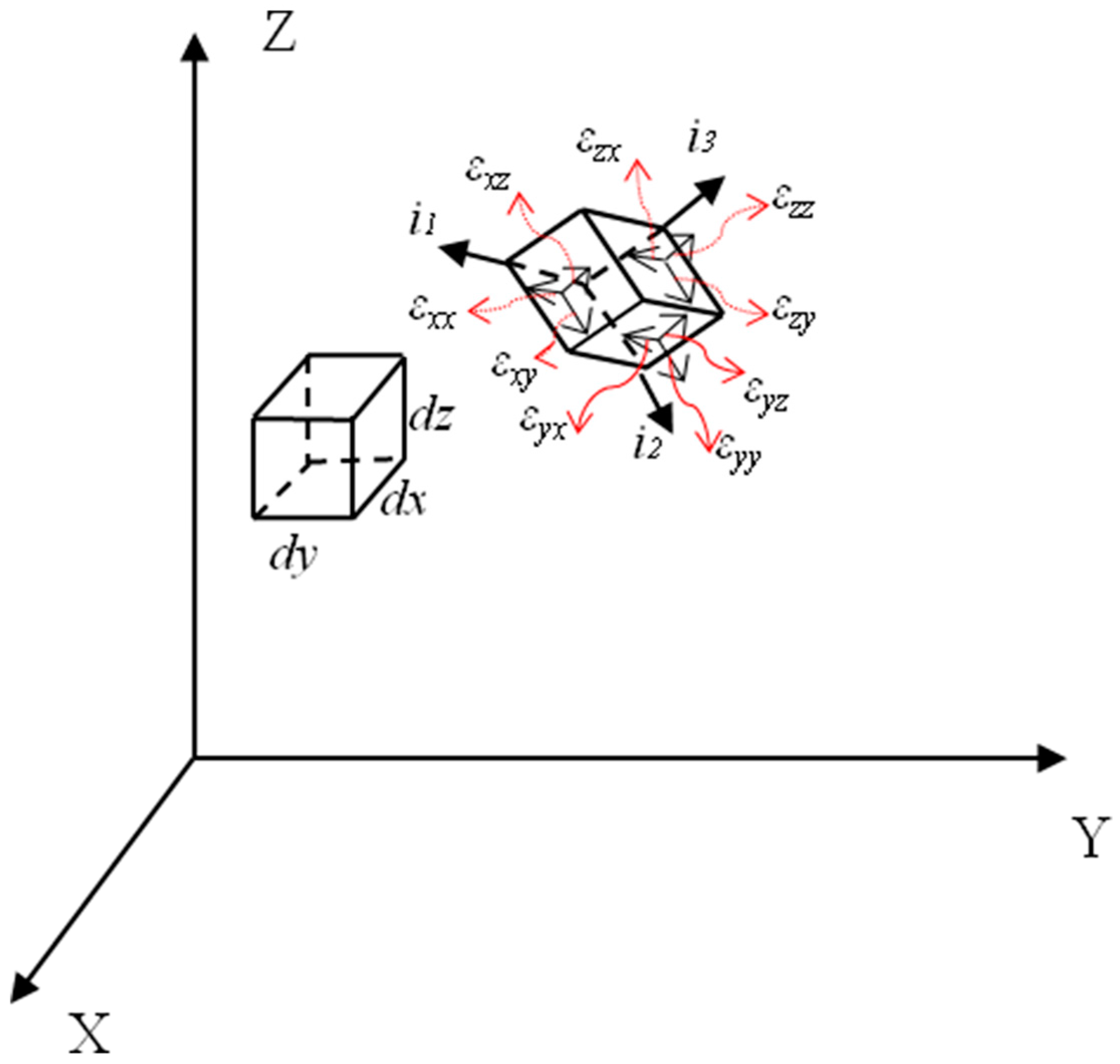
13], strain and plastic work may be calculated by reference to an element, the deformed volume, which is:
where
εxx,
εyy,
εzz are the tensorial strains in different directions.
The deformed volume is equal to the product of the undeformed volume
dx,
dy,
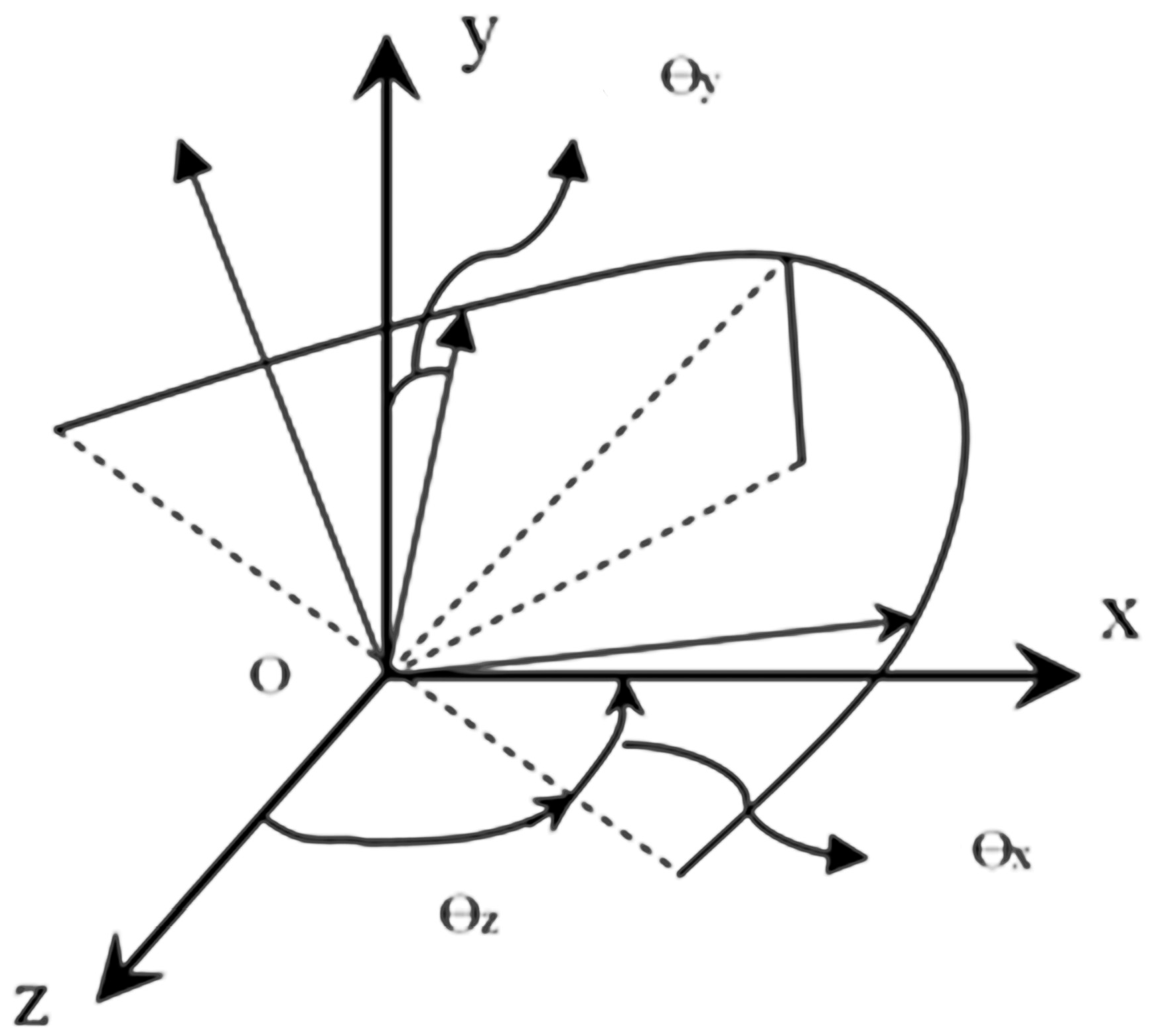
dz and a function of the six strain components. The form of this function depends on the physical properties of the dimensions and shape of the body. Alternatively, the strain components can be expressed in terms of the three principal strains
ε1,
ε2,
ε3 and the direction cosines of the principal axes of strain
ε1,
ε2,
ε3 with respect to the X, Y and Z axes. Thus, the direction cosines might be regarded as a function of three independent quantities, the Euler angles (
Figure 1)
θ,
ϕ,
Ψ which determine the orientation of the trihedral
ε1,
ε2,
ε3 relative to the trihedral X, Y and Z. Therefore,
dA can be written as:
The three independent invariants
ε1,
ε2,
ε3 are important, as they have a simple physical meaning, individually, in the case of small deformations. The strain components can be expressed by
a0,
a1,
a2 factors, and thus it is more expedient to indicate the work of deformation on an element of an isotropic body as a function of the three invariants
a0,
a1,
a2:
Thus, the induced work by considering the possible deforming of an elementary parallelepiped of an isotropic body can be calculated by:
Therefore, for the entire body:
where the integration extends over the volume of the body in its unstrained state, as
dxdydz is the volume of an elementary parallelepiped in that state. The function Φ(
a2,
a1,
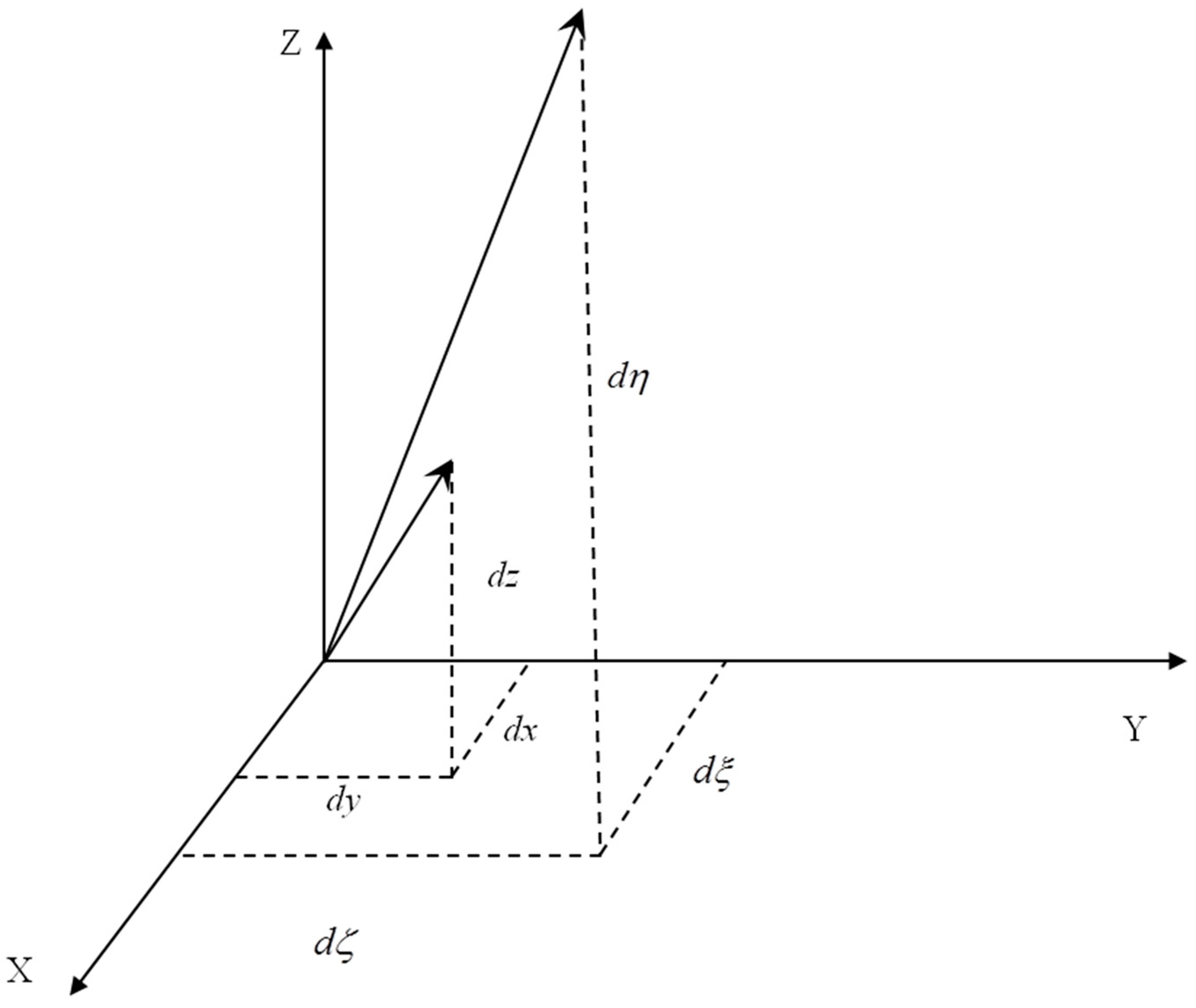
a0) is the strain energy of a unit volume of the body in its unstrained state, specific strain energy. To calculate all of the possible induced energy inside the entire element due to the different deformations in the different directions, the application of the principle of virtual displacement to a deformed body in a state of equilibrium is considered. The arbitrary vectors including
,
and
were assigned to the displacements and
dξ,
dζ,
dη are virtual displacement (
Figure 2), respectively, which can be considered as arbitrary continuous functions of
x,
y, z equal to zero at those points where the values of the displacement are known.
Thus, the rate of change strain energy will be in line with
δA, where it would be equal to the work done by all the exterior forces applied to the body in affecting the indicated virtual displacement (
Figure 3). Thus,
δA can be written by:
where
δR1 is the virtual work due to the body forces and
δR2 is the virtual work done by the surface forces. The virtual work done by the body forces is equal to:
where
are the components along the X, Y, Z axes of the force referred to as a unit volume of the deformed body,
dxdydz is the volume element of the unstrained body, and
Ddxdydz = (
V*/
V)
dxdydz is the corresponding volume element of the strained body:
where
are the components along the X, Y, Z axes of the force acting on a unit area of the surface of the deformed body, while
dΩ’ is the differential of the area in the strained state.
To calculate
δR2 over the surface of the body in its strained state, it would be possible to replace
dΩ’ in terms of
dΩ, the differential of surface area in the unstrained state by considering an elementary rectangular area with sides
on the bounding elementary rectangle has an area equal to
d and the relevant orientation can be determined by the direction of the unit normal vector
. Thus, as a result of the deformation, the rectangular area is transformed into a surface of the deformed body having the form of a parallelogram with sides (1 +
Ea)
da, (1 +
Eb)
db. The cosine of the angle formed by these sides is:
where
Ea,
Eb are the relative elongations in the directions
da,
db and
εaa,
εbb,
εab are the corresponding tangential strain components. Therefore, an element on the surface of the strained body has an area equal to:
The coefficient
which is equal to the ratio of the elements of area in the terminal and initial states can be expressed in terms of the strain components relative to the X, Y, Z axes and the three direction cosines of the normal to the surface in the unstrained state. Thus, it is necessary to replace the strain components
εaa,
εbb,
εab in the formula:
by their expressions in terms of
εxx, …,
εyz and the direction cosines of
da,
db and
n, then, by considering the relevant transformations:
and
are the direction angles of the normal to the bounding surface in the unstrained state relative to the X, Y, Z axes. The virtual work done by the external surface through the virtual displacements
δu,
δv,
δω is of the form:
where
is the area of a surface element in the initial state. Thus, in order to calculate the value
δR2, the integration should be carried out over the surface in the unstrained state. The key parameters
can be also calculated based on the Euler-Bernoulli beam model Ranzi and Gilbert [
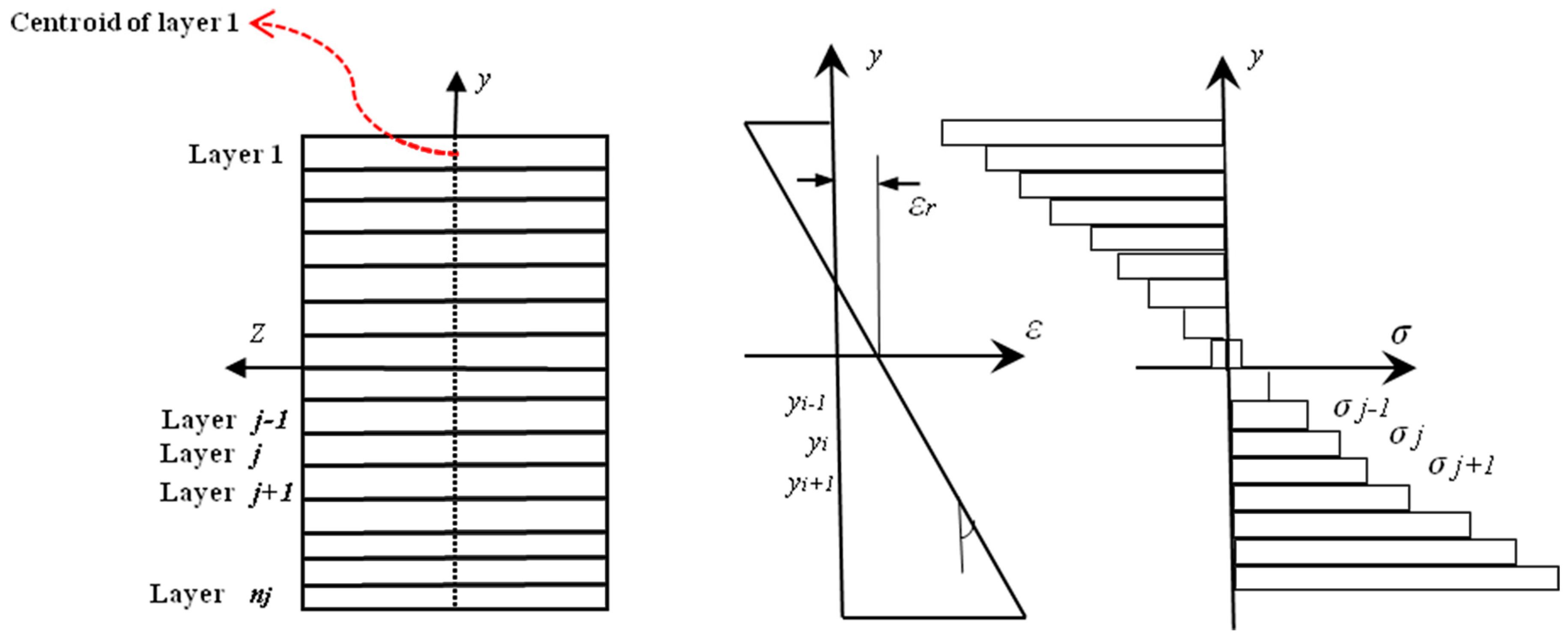
14]. An analytical method is developed to evaluate shear stress and strain distributions between the engaged surfaces throughout different joint layers by considering the beam theory method in different directions with respect to the different planes, where it can independently calculate shear forces between the different layers and shear strain as well as the curvature distribution along the different layers that have been extracted. The main concept to derive the following equations was extracted from Ranzi and Gilbert [
14] and Ranzi et al. [
15]. According to Ranzi and Gilbert [
14], the cross-sectional (
Figure 4) analysis is based on the assumption of the Euler-Bernoulli beam model.
The strain distribution across the section can be calculated by
ε =
εr −
y ×
κ where
εr is the strain at the reference point (which can be determined at any point),
y is the distance between the selected point and location of the neutral axis of the cross-section and
κ is the curvature across the section in different strata layers. A vector can be introduced by
K(
D) which will be included in the internal action
N (axial forces) and
M (internal moment). External loads, which might be due to the effect of the self-weight of the strata layers as well as the possible applied forces due to the vertical or horizontal displacement in the different layers, can induce the external axial force
Ne, external moment
Me and
dA is the differentiate of the engaged surfaces. The relationship between the internal and external actions can be presented by:
By considering the nonlinear interactions, the presented equations can be re-written by:
All the equations can be re-presented in matrix format:
The partial derivatives of
N and
M with respect to
εr and
κ can be re-arranged in a:
more practical form, recalling the definitions of internal actions as:
where the values of the stress depend on the constitutive models adopted for the materials and on the magnitude of the strain [
14]:
Thus, by calculating stress and strain at the different points at the different layers of the overburden, the internal axial forces as well as internal moments can be calculated. It was assumed that strain energy (
A) can be calculated by:
Furthermore:
where, in accordance with the former equations and substituting for
a0,
a1 and
a2 according to Equations (4)–(6),
and similarly for
εyy and
εzz, furthermore:
and similarly for
εxz and
εyz. Moreover, by taking into account:
and similarly for
εyy and
εzz, furthermore:
and similarly for
εxz and
εyz. And by substituting these values of
:
and similarly for
uy,
uz;
vy,
vz and
wy,
wz. Thus, the strain energy (
A) can be calculated by:
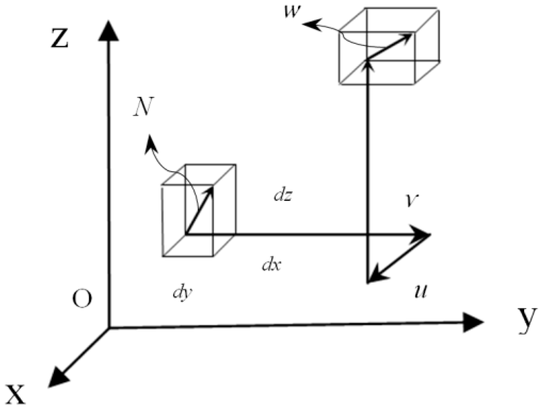
where
σxx ×
εxx, …,
σyz ×
εyz (
Figure 5) can be calculated according to the principal of the virtual work and virtual deformation
δA =
δR1 +
δR2 when the induced stresses and strains cannot be directly extracted from the simulated model.
3. Calculating the Released Energy
Initially, in order to calculate the released energy, an assumption was made based on the principle of thermodynamics. The accuracy of the assumption is validated in line with the analytical model validation. Provided that there is an exponential relationship between the changing rate of the released energy as well as the changing rate of the strain energy and the joint density per unit volume of a sample, thus
α is the significant coefficient where it can represent the rating of the differences between the released and strain energy over the changing rate of the strain energy with respect to the total strain:
It can be represented by:
where
A is the strain energy and
,
are the strain energy in the different increments,
is the damping factor
and
D is the joint density per unit volume of the sample. Also,
and
are the released energy in the different increments. Besides,
where it is the strain component in all of the directions. Thus, we have:
Furthermore, it is clear that:
Provided that we assume that the constant values are
C1 = 0,
C2 = 0 based on the initial conditions:
By integrating in both parts of the equations:
Provided that we assume that the constant values are
C3 = 0,
C4 = 0 based on the initial:
Equation (77) is the significant equation to calculate the amount of the released energy based on the value of the strain energy. The suggested equation can indicate the relationship between the released energy as well as the strain energy due to different joint density per unit volume of a sample as well as the damping coefficient. Developing the current equation is the major contribution of the paper. It can also help calculate the amount of the released/dissipated energy as well as help determine zones of high risk of coal bursts.
5. Discussion of the Results
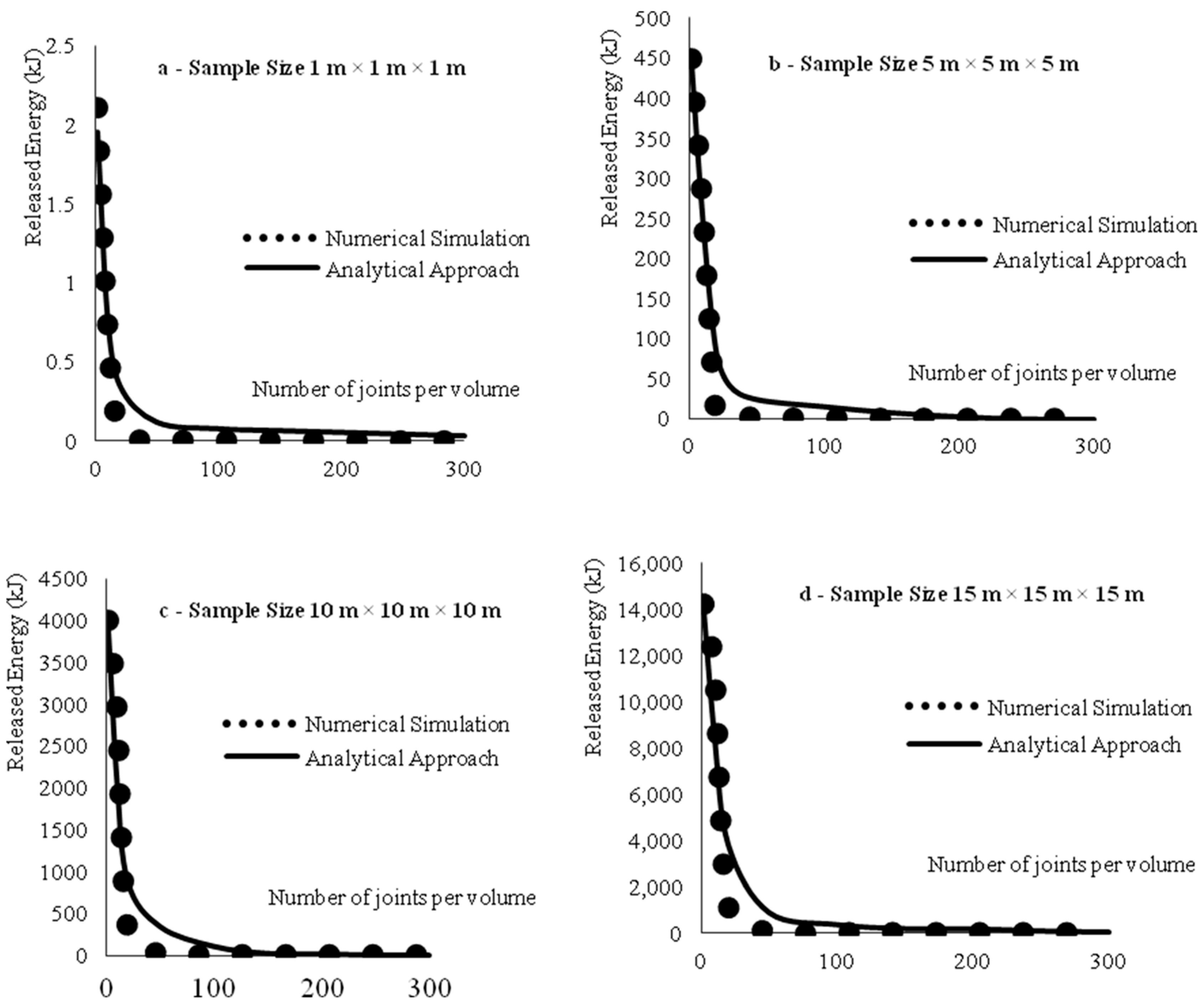
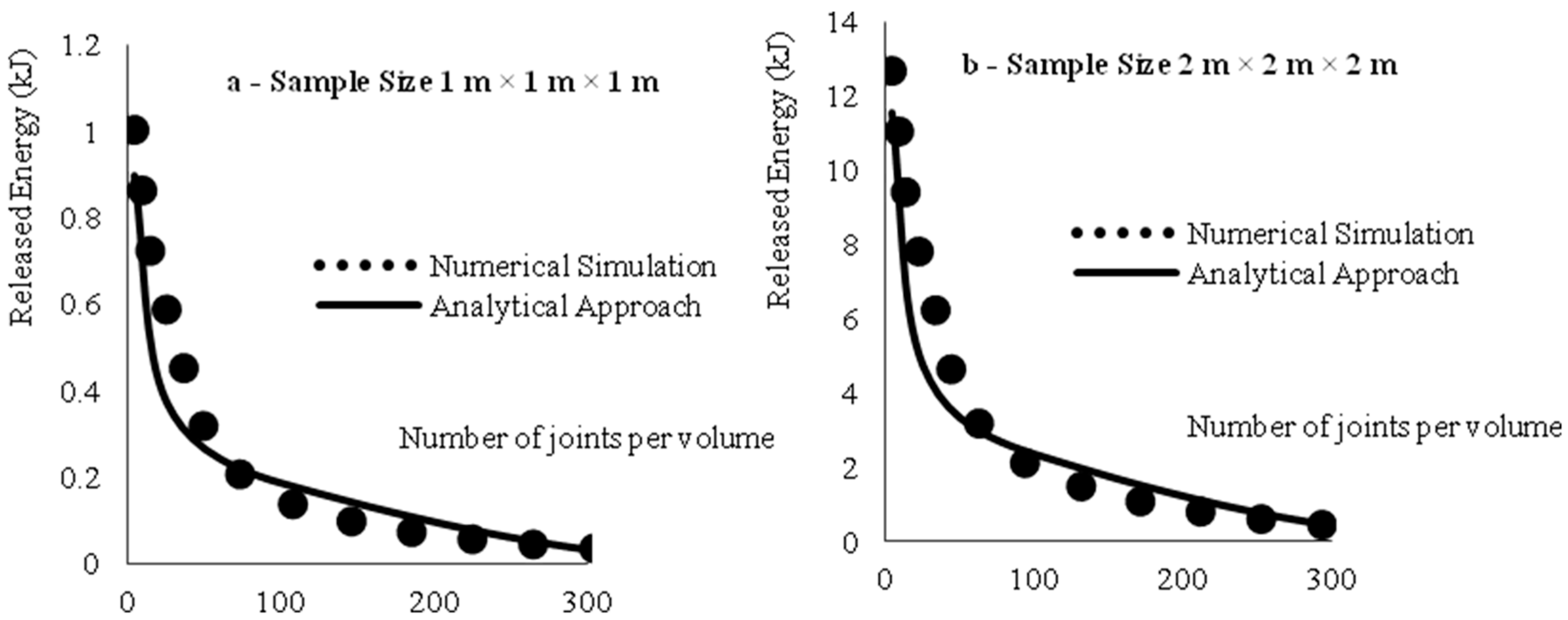
Figure 7 presents the estimated amount of released energy in different coal samples with different joint densities using both the analytical and numerical methods. As illustrated, there is a good agreement between the numerical and analytical solutions. As the number of joints increases, the amount of the released energy in the simulated coal samples significantly decreases. This is due to the effect of the physical and damping interaction between the engaged surfaces of the joints which creates an internal released energy. It is also found that by increasing the number of joints, the global integrity of the simulated samples is considerably reduced, which may lead to reducing the amount of released energy in the coal.
Existing rock and coal discontinuities can seriously affect the mechanical properties of coal materials. Research on the behaviour of coal discontinuities has been carried out in line with studies of the behaviour of coal properties. Knowledge of the behaviour of geological discontinuities such as joints and faults is essential for understanding slip-type coal bursts. One important aspect of the behaviour of a joint is its deformability. The discussed approach can lead to a sound understanding of the impact of coal local mechanical properties on energy released or absorbed.
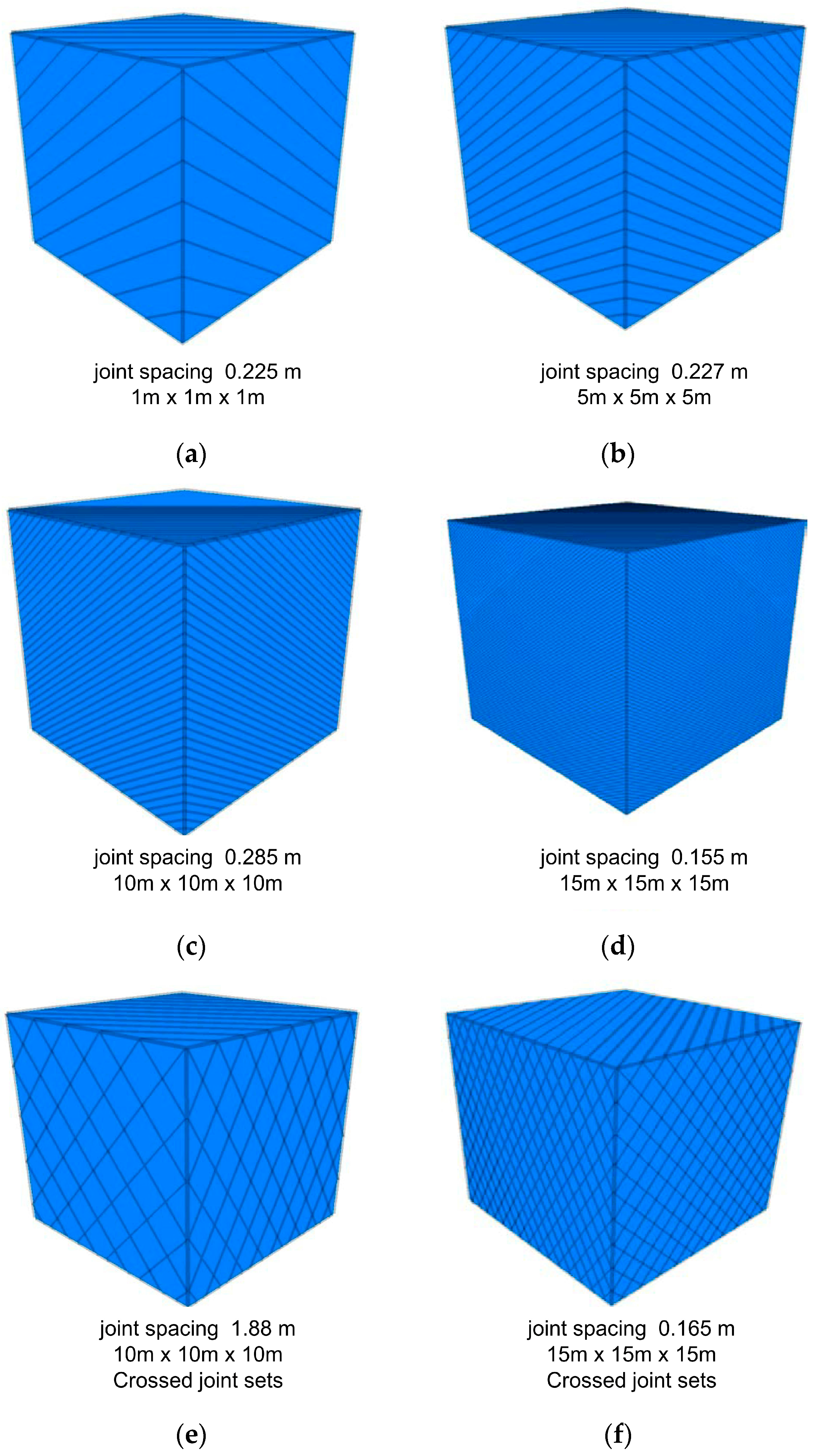
Figure 8 presents a comparison between the suggested analytical solution and the numerical simulation while considering different crossed joint set densities.
Based on the observed results from
Figure 6, a proper agreement can be found between the discussed analytical solution and the numerical simulation. More realistic and complex conditions, such as multiple, intersecting coal discontinuities under the influence of sequential mining operations, can also be studied based on the established methodologies and validated numerical program. By comparing the single joint results against crossed joints, it is shown that the developed analytical model has better prediction for the crossed joints condition. As the density of the joints increases in multiple directions, the condition in the numerical models comes close to the proposed assumption in the suggested closed form solution. According to the inductive approach, it proves the reliability of the initial hypothesis where there is an exponential relationship between the changing rate of the released energy as well as the changing rate of the strain energy and the joint density per unit volume of a sample. The current research developed a number of innovative analytical and numerical techniques and has advanced the current knowledge of energy calculations applied to coal bursts. In general, energy release in coal mining can occur passively in the form of heat and sound or dynamically in the form of coal bursts. The sudden energy release values are related to the energy changes in the materials that take place between mining steps. For the vast majority of elements, energy changes are associated with changes in the element’s stress and deformation state while staying on the same material curve.
It was also hypothesised that energy calculations may provide a strong extrapolative capability to determine the possible location and timing of a coal burst. However, from past experiences documented in the literature, it appears that coal burst prediction based on energy calculations has practical limitations due to the extreme sensitivity of the energy calculations to the value of uncertain input parameters. This sensitivity of the calculated energy results to the input properties of the geologic material may reflect the true situation underground where small anomalies in geology or rock properties may ultimately determine the precise location and timing of coal burst. Nevertheless, this sensitivity of the energy calculations to uncertain material properties appears to be a practical limitation to forecasting coal bursts using calculated energy values. Obtaining sufficient geological data, such as properties of roof and floor strata, stress fields and properties and locations of existing rock discontinuities, can improve the quality of analyses of unstable failures in underground mining. Due to the lack of relevant geological data, performing an analytical and a numerical simulation can be classified as a good tool to improve the understanding of rock and coal mass behaviour against possible abnormal loading. The established methodologies can be extended in more detail in three-dimensional modelling. With three-dimensional models, back analyses of unstable failures in historical cases can be performed to calibrate the parameters in the models. The calibrated models may be able to provide useful information about possible locations and intensities of unstable failures in future mining operations and prevent serious coal bursts from occurring. Different coal burst proneness indexes were suggested by different researchers [
16]. Xie et al. [
16] indicated that dissipated and released energy can play a significant role. A sudden release of the strain energy may lead to a catastrophic failure, which clearly indicates a certain condition where the coal mass collapses. Based on the failure mechanism, the fracture procedure of a coal mass might be started from a partial fracture which would be followed by local damage. This procedure will be finally resulting in collapsing the mining structures. The failure process is thermodynamically permanent, which includes released and dissipated energy. By calculating released energy, it is possible to calculate the amount of dissipated energy which can help calculate different energy index impact factors. This is a significant step towards forecasting coal burst-prone zones and reducing threats to safety and production.


