Abstract
With plenty of parallel inverters connected to a weak grid at the point of common coupling (PCC), the impedance coupling interactions between the inverters and the grid are enhanced, which may cause high-frequency harmonic oscillation and further aggravate the system instability. In this paper, a basic technique for inverter output impedance is proposed to suppress the oscillation, showing that the inverter output impedance should be designed relatively high at the harmonic oscillation frequency, while relatively low at other frequencies. On the basis of the proposed technique, two virtual impedances are added to be in parallel and in series with the original inverter output impedance, respectively. Thus, an oscillation suppression method by two notch filters is proposed to realize the virtual impedances and increase the whole system damping. The implementation forms of the virtual impedances are presented by the proposed PCC voltage feedforward and grid-side inductor current feedback with two notch filters. Finally, simulation and experimental results are provided to verify the validity of the proposed control method.
1. Introduction
With the increasing energy crisis and environmental problems, renewable energy generation, mostly in power plants or microgrids, have grown rapidly [1,2,3]. Due to the distributed locations of renewable energy generators, multiple transformers and long transmission lines are utilized to connect the systems to the public grid [4]. Thus, the public grid exhibits the feature of a weak grid in which grid impedance cannot be ignored [5].
Especially, in a large-scale power plant or microgrid, renewable energies are mostly connected to the grid via parallel inverters [6,7]. By this way, the power plant or microgrid can easily expand the output power capacity, and it is also convenient to connect plenty of renewable energies into the grid [8]. Under weak grid conditions, the impedance coupling interactions between the inverters and the grid are enhanced further due to grid impedance [9]. If control parameters and device selection of all inverters are the same, the grid impedance seen by each inverter will become n times of the real grid impedance [10]. Therefore, these interactions may cause oscillation if inverters are improperly designed or controlled.
There are two methods to analyze the system’s stability. The first is the eigenvalue-based analysis [11], which is usually utilized to evaluate the system’s stability. The eigenvalue-based stability analysis studies the eigenvalues of a system’s state space model matrix, which requires the physical features and control parameters in the system [12]. The second one is the impedance-based stability criteria [13,14], which is well built to adjudicate the system stability. The system will be stable if two requirements are satisfied [13]. The first requirement is that the grid-connected inverter is stable in the public grid, and the other is that the product of grid impedance and inverter output admittance satisfies the Nyquist criterion. The industrial and academia community have widely accepted the theory of impedance-based stability analysis [15,16].
Some strategies were proposed to suppress the oscillation, which can be divided into two cases. One is to introduce additional hardware equipment to the PCC [17], the other is to reshape the inverter output impedance [18,19,20,21,22,23]. Adding additional equipment was adopted to stabilize the paralleled multi-inverter system, in which structures and control parameters of the inverters are unknown. Reference [17] installed an active damper at the PCC to suppress the oscillation. However, extra cost may exist owing to the demand of additional circuitry [24].
Different impedance reshaping methods need to be adopted to suppress the oscillation. The existing impedance reshaping methods mainly include: capacitance-current-feedback methods [18,19], capacitance-voltage-feedback methods [20,21], and virtual resistor methods [22,23]. In Reference [18], the real-time computational method was proposed to decrease the computational delay, which can simplify the design and enhance the performance. However, if the grid voltage has much harmonics, it will make the duty cycle of the inverters change sharply. Similar to the capacitance-current-feedback methods, useful active damping was induced by the derivative feedback of the capacitance voltage [20,21]. However, the capacitance-voltage-feedback methods should handle the challenge of grid voltage variation. In References [22,23], the virtual resistor methods made the inverter output impedance show high impedance at all frequencies, which can suppress the oscillation. However, due to the high impedance characteristics of the inverters at the fundamental frequency, the methods will cause the change of the fundamental current, and then influence the tracking precision of the grid-connected power. Therefore, the fundamental impedance and high-frequency harmonic impedance of inverters are separately considered. The fundamental impedance should be designed as the low impedance, which does not affect the grid-connected power tracking. However, the high-frequency harmonic impedance is designed as the high impedance to suppress the oscillation.
In this paper, the oscillation suppression method by two notch filters is proposed to increase the whole system damping. This paper is organized as follows. Section 2 analyzes the oscillation mechanism of a paralleled multi-inverter system. Section 3 presents the demand for the inverter output impedance for the purpose of oscillation suppression, and the method of adding the virtual impedances to meet the demand is proposed, which introduces two notch filters to the PCC voltage feedforward and grid-side inductor current feedback. Section 4 compares and analyzes the system’s stability in two cases. Section 5 and Section 6 provide the simulation and experimental results to verify the validity of the proposed control method. Finally, Section 7 gives the conclusion.
2. Oscillation Mechanism of Paralleled Multi-Inverter System
2.1. System Description
The structure of a paralleled multi-inverter system is shown in Figure 1. The left and right side are the inverter subsystem and the grid subsystem. j = 1, 2, …, n. Udc is the DC voltage. uinvj, uC1j, and uPCC are the inverter output voltage, filter capacitor voltage, and PCC voltage. ug is the grid voltage. Zg is the grid impedance. Inductor-capacitor-inductor-type (LCL-type) filter is constituted by the inverter-side inductor L1j, grid-side inductor L2j, and filter capacitor C1j. RL1j and RL2j are parasitic resistances of L1j and L2j. iL1j is the inverter-side inductor current. iC1j is the filter capacitor current. ioj is the grid-side inductor current. ig is the grid-connected current.
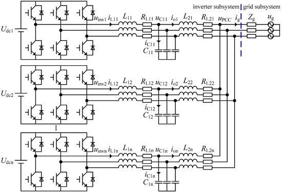
Figure 1.
Structure of paralleled multi-inverter system.
2.2. Oscillation Mechanism
In the grid-connected mode, single inverter is equivalent to the current source ij in parallel with equivalent admittance Yj, which is the Norton equivalent circuit [23]. The grid is equivalent to the grid voltage ug in series with grid impedance Zg. From the PCC, the Norton equivalent circuit of paralleled multi-inverter system is shown in Figure 2a. From Figure 2a, the circuit relationship about uPCC is shown in Equation (1) by the nodal analysis method.
where ij is the current source of a single inverter, and Yj is the equivalent admittance of a single inverter.
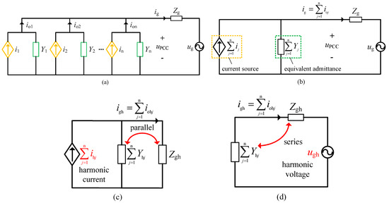
Figure 2.
Output admittance model and oscillation mechanism of paralleled multi-inverter system. (a) Norton equivalent circuit; (b) Output admittance model; (c) Parallel oscillation; (d) Series oscillation.
From Equation (1), the output admittance model of paralleled multi-inverter system satisfies the Equation (2), as depicted in Figure 2b.
The frequency of harmonic current ihj is caused by the system nonlinear factor. If it is equal to or close to the parallel resonance frequency of impedance network, it will cause the parallel oscillation, as shown in Figure 2c. The frequency of harmonic voltage ugh is caused by the grid distortion. If it is equal to or close to the series resonance frequency of impedance network, it will result in the series oscillation, as shown in Figure 2d.
From Figure 2b, the grid-connected current ig can be derived as
where the product of grid impedance and inverter output admittance is defined as the impedance ratio K, which can be expressed as
From Equation (3), it can be assumed that the grid voltage is stable in the absence of the inverter, and the inverter will be stable if the grid impedance is zero. Nevertheless, when the grid impedance is not negligible, the system will be stable only if the impedance ratio K satisfies the Nyquist criterion in Reference [12]. In other words, the system will be stable, only if the Nyquist curve of the impedance ratio does not surround (−1, j0).
Thus, there are impedance coupling interactions between the inverters and the grid, which will aggravate the harmonic distortion of grid-connected current, lead to the oscillation in paralleled multi-inverter system, and even cause the system to be unstable.
3. Oscillation Suppression Method by Two Notch Filters for Parallel Inverters
3.1. Demand for the Inverter Output Impedance
To suppress the oscillation, the inverter output impedance should be designed relatively high at the harmonic oscillation frequency while relatively low at other frequencies. For this purpose, the virtual impedances are added to be connected with the original output impedance, as shown in Figure 3. Figure 3a–c presents parallel, series, and parallel-series virtual impedances, respectively. The above three forms can reach the same performance for oscillation suppression. For the first and second forms, it is relatively complicated to introduce one virtual impedance to realize that the inverter output impedance shows high at the harmonic oscillation frequency while relatively low at other frequencies. However, the third form with two virtual impedances is relatively easy to achieve this purpose. Thus, the third form is mainly discussed in this paper.
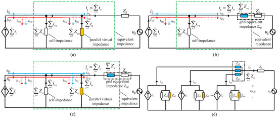
Figure 3.
Equivalent schematic diagram. (a) Parallel virtual impedance; (b) series virtual impedance; (c) parallel-series virtual impedances; (d) equivalent output impedance model.
In Figure 3c, Zoj is the self-impedance when the parallel-series virtual impedances are not added. The equivalent impedance Zj (Zj = 1/Yj) is formed by Zoj in parallel with Zpj, and then in series with Zsj. The grid equivalent impedance Zsgj consists of the virtual impedance Zsj and the grid impedance Zg connected in series. if/hj, if/h1j, if/h2j, and if/h3j are total fundamental/high-frequency harmonic current, fundamental/high-frequency harmonic current of Zoj branch, fundamental/high-frequency harmonic current of Zpj branch, and fundamental/high-frequency harmonic current of Zsgj branch, respectively. if/hj = if/h1j + if/h2j + if/h3j. The total fundamental frequency current ifj and the total high-frequency harmonic current ihj are determined by the shunt circuit, consisting of the self-impedance Zoj, parallel virtual impedance Zpj, and grid equivalent impedance Zsgj. From the PCC, the Norton equivalent circuit of Figure 3c is refined into the forms of Figure 3d.
On the basis of the proposed basic technique, the parallel virtual impedance Zpj should be designed to show low impedance at the harmonic oscillation frequency. By doing so, most high-frequency harmonic current will flow into the parallel virtual impedance Zpj branch; it effectively suppresses the oscillation of paralleled multi-inverter system. In the meantime, to improve the power quality of grid-connected current, the series virtual impedance Zsj should be designed to display low impedance at the fundamental frequency. This way, most fundamental frequency current flows into the grid branch with relatively low impedance.
3.2. Oscillation Suppression Method
The parallel-series virtual impedances in Figure 4 can be realized by introducing two notch filters. In Figure 4, two virtual impedances are added in parallel and series with inverter output impedance, respectively. Gi is the grid-connected current loop proportional resonant (PR) controller, GPWM is the equivalent gain of the inverter, ZL1j = sL1j + RL1j, ZC1j = 1/sC1j, ZL2j = sL2j + RL2j.
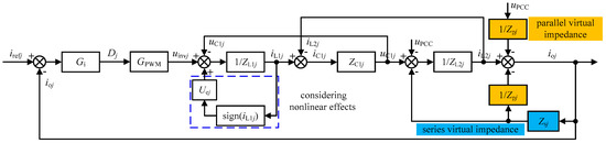
Figure 4.
Equivalent control block diagram of oscillation suppression method by two notch filters for parallel inverters.
The parallel virtual impedance Zpj and series virtual impedance Zsj can be expressed as
where r1 and r2 are the proportional coefficient and GN is the notch filter.
The grid-connected current loop PR controller Gi can be expressed as
where kp is the proportional coefficient of quasi-proportional resonant controller, ki1 is the resonance gain of quasi proportional resonance controller, ωc is the cut-off angular frequency, and ωo is the fundamental angular frequency.
The effects of dead-time of switching devices in paralleled multi-inverter system are regarded as a disturbance, which have a constant amplitude and an alternative direction depending on the inverter-side inductor current iL1j [25]. It is notable that the disturbance can be seen as the controlled current source idj in Norton equivalent circuit, which can be presented as
where and .
According to Reference [25], Uej in Equation (7) can be expressed as
where UTj and UDj are the on-state voltage drop of switching devices and diodes, Tsj, tdj, tonj and toffj are switching period, dead-time, turn-on time, and turn-off time of switching devices.
Meanwhile, sign(iL1j) in Equation (7) can be expressed as
From Figure 4, the closed-loop transfer function of the system can be expressed as
where irefj is the reference current of single inverter, Gj is the current source equivalent coefficient of single inverter, and Yj is the equivalent admittance of single inverter.
According to Equation (10), the refined equivalent output impedance model is shown in Figure 5. The current source ij is equivalent to the current source i1j in parallel with the current source idj. Two virtual impedances are added to be in parallel and in series with the original inverter output impedance, respectively. Thus, Figure 5 is equivalent to the refinement of Figure 3d, which can achieve the proposed approach.
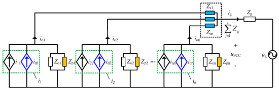
Figure 5.
Refined equivalent output impedance model.
From Figure 5, the equivalent model of the m-th inverter can be expressed as
where irefm, Gm, Ym, idm, ZL1m, ZC1m, ZL2m, Zpm, and Zsm are the variables of the m-th inverter.
Substitute Equation (1) into Equation (11), and Equation (11) can be rewritten as
where Gselfm is the transfer relationship between the grid-side inductance current iom of the m-th inverter and reference current irefm of the m-th inverter, Gparalm,j is the transfer relationship between the grid-side inductance current iom of the m-th inverter and reference current irefj of the jth inverter, and Gserim is the transfer relationship between grid-side inductance current iom of the m-th inverter and grid voltage ug.
When a similar analysis method is adopted to other inverters, the system can be expressed using a closed-loop transfer function matrix with reference currents, grid voltage and controlled current sources as inputs and grid-side inductor currents as outputs
It is obvious that the strong coupling between the inverters and the grid may exist and introduce harmonic oscillation currents under weak grid condition.
According to Figure 4, Figure 6 gives the control block diagram of the oscillation suppression method by two notch filters for parallel inverters. The first notch filter is introduced into the feedforward path of PCC voltage and the second notch filter is introduced into the feedback path of the grid-side inductor current. The feedback path of the grid-side inductor current with the notch filter is equivalent to a virtual impedance in series with inverter output impedance, which can effectively improve the power quality of the grid-connected current. The feedforward path of PCC voltage with the notch filter equals to a virtual impedance in parallel with inverter output impedance. This can effectively restrain the parallel inverters’ harmonic current from flowing into the grid and avoid the oscillation phenomenon. H1j is the feedback coefficient of the grid-side inductor current, and H2j is the feedforward coefficient of PCC voltage.
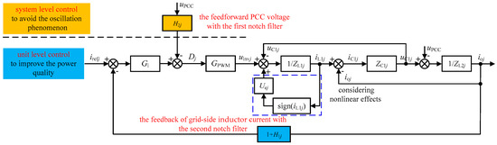
Figure 6.
Control block diagram of the oscillation suppression method by two notch filters for parallel inverters.
From Figure 6, the equivalent closed-loop transfer function of the system can be expressed as
where Gjeq is the equivalent coefficient of the current source after the single inverter transformation, Yjeq is the inverter equivalent admittance after the single inverter transformation, , , and .
In order to achieve the same purpose of Figure 4 and Figure 6, the equivalent coefficient of the current source and the inverter equivalent admittance in Equation (10) are equal to those in Equation (14). Thus, it can be expressed as
From Equation (15), the feedback coefficient of the grid-side inductor current H1j and the feedforward coefficient of PCC voltage H2j can be expressed as
At the specific frequency, the amplitude of the notch filter is greatly attenuated while the amplitude at other frequencies is almost non-destructive. The notch filter GN can be expressed as
where fo is the fundamental frequency and Q is the quality factor of the notch filter.
The analysis diagrams of the notch filter with Q = 0.25, 0.5, and 1 are shown in Figure 7. From Figure 7a, the larger Q is, the better the notch characteristic of the notch filter, but the worse the frequency adaptability. From Figure 7b, when Q = 0.25, the characteristic equation has two unequal real poles on the negative real axis of the s plane, which is over-damping. When Q = 0.5, the characteristic equation has two equal real poles on the negative real axis of the s plane, which is critical-damping. When Q = 1, the characteristic equation has the conjugate complex poles on the left half plane, which is under-damping. From Figure 7c, the tuning time of notch filter with Q = 0.5 is better than Q = 0.25, 1. Therefore, considering the notch characteristics and dynamics comprehensively, the Q value was selected to be 0.5.
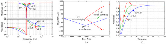
Figure 7.
Analysis diagrams of notch filter with Q = 0.25, 0.5, 1. (a) The Bode diagram of notch filter; (b) Pole-zero plot of notch filter; (c) Unit step dynamic responses of notch filter.
The Bode diagrams of parallel virtual impedance Zpj and series virtual impedance Zsj are shown in Figure 8. At the fundamental frequency, the parallel virtual impedance Zpj shows a high impedance, and the series virtual impedance Zsj displays a low impedance, so that the fundamental current flows into the grid. At the high frequency, the parallel virtual impedance Zpj shows a low impedance, and the series virtual impedance Zsj displays a high impedance, so that the high-frequency harmonic current flows into the parallel virtual impedance Zpj branch.
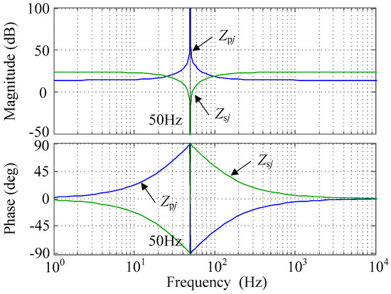
Figure 8.
The Bode diagrams of parallel virtual impedance Zpj and series virtual impedance Zsj.
The Bode diagrams of the inverter self-impedance Zoj, parallel virtual impedance Zpj, grid equivalent impedance Zsgj, and grid impedance Zg are shown in Figure 9. Combined with Figure 5, the grid equivalent impedance Zsgj is much lower than the self-impedance Zoj and the parallel virtual impedance Zpj at the fundamental frequency, thus most fundamental frequency current flows into the grid branch with relatively low impedance, which improves the power quality of grid-connected current. At the high frequency, the parallel virtual impedance Zpj is much lower than the self-impedance Zoj and grid equivalent impedance Zsgj, thus most high-frequency harmonic current flows into the parallel virtual impedance Zpj branch with relatively low impedance, and it effectively suppresses the oscillation of the paralleled multi-inverter system.
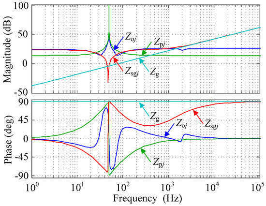
Figure 9.
The Bode diagrams of the inverter self-impedance Zoj, parallel virtual impedance Zpj, grid equivalent impedance Zsgj, and grid impedance Zg.
4. Contrast Analysis of System Stability under Weak Grid Condition
In order to compare and analyze the system stability, different conditions of adding parallel-series virtual impedances are shown in Table 1. Parallel virtual impedance Zpj = r1 and series virtual impedance Zsj = r2, abbreviated as case I. Parallel virtual impedance Zpj = r1/GN and series virtual impedance Zsj = r2GN, abbreviated as case II (proposed control method).

Table 1.
Different conditions of adding parallel-series virtual impedances.
To verify that the system satisfies the precondition of using the Nyquist criterion, the open-loop Bode diagrams and closed-loop pole-zero diagrams of the equivalent coefficient of current source Gjeq for single inverter in different cases are shown in Figure 10. From Figure 10a,b, it can be seen that the gain margin (GM) and the phase margin (PM) are greater than 0, no right half-plane pole exists, and the single-inverter system is in a stable state. Therefore, the system satisfies the precondition of using the Nyquist criterion. The stability condition of the paralleled multi-inverter system is that the Nyquist curve of the impedance ratio does not surround (−1, j0).
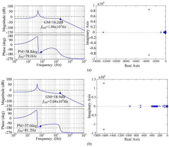
Figure 10.
The open-loop Bode diagrams and closed-loop pole-zero diagrams of the equivalent coefficient of current source Gjeq for single inverter in different cases. (a) Case I; (b) Case II.
Figure 11 shows the Nyquist diagrams of impedance ratio K for the paralleled multi-inverter system. From Figure 11a, when the number of inverters is 2, 3, 4, 5, and 6, respectively, the Nyquist curve does not surround (−1, j0) in case I, and the system is in a stable state. However, when the number of inverters is 7, 8, 9, 10, and 11, respectively, the Nyquist curves all surround (−1, j0), and the system is in an unstable state. However, from Figure 11b, regardless of the number of inverters, the Nyquist curves would never wrap around (−1, j0) in case II, and the system is in a stable state. Therefore, compared with case I, the proposed oscillation suppression method by two notch filters can effectively restrain parallel inverters’ harmonic current from flowing into the grid, and avoid the oscillation phenomenon.
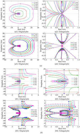
Figure 11.
Nyquist diagrams of impedance ratio K for the paralleled multi-inverter system. (a) Case I; (b) Case II.
5. Simulation Verification
To verify the correctness of theoretical analysis, the simulation model of a paralleled multi-inverter system was built based on Figure 1. Several cases including two and seven inverters were simulated by PSIM (Powersim Inc., Rockville, MD, USA) simulation. The system parameters are shown in Table 2.
Table 2.
System parameters.
When two inverters were connected to a weak grid in case I and case II, the root mean square (RMS) value of the reference grid-side inductor current irefm for each grid-connected inverter increased from 18.75 A to 37.5 A at 0.405 s. Therefore, the RMS of the reference grid-connected current igref increased from 37.5 A to 75 A for the two parallel inverters. Simulation results of the grid-connected current with two parallel inverters are shown in Table 3.
Table 3.
Simulation results of grid-connected current with two parallel inverters. THD: total harmonic distortion.
In case I, the transient simulation waveforms of PCC voltage uPCC and grid-connected current ig are depicted in Figure 12a,b. It can be seen that the distortion rate of PCC voltage uPCC is 1.57%. The grid-connected current ig and corresponding spectrum from 0.30 s to 0.36 s are shown in Figure 12c,d, which describes the situation before the reference current surges. The distortion rate of grid-connected current ig is 6.07%, the resonance point is near the 25th harmonic (1250 Hz), and the resonance peak is 1.77 A. The grid-connected current ig and corresponding spectrum after the reference current suddenly increases are shown in Figure 12e,f. The distortion rate of grid-connected current ig decreases to 3.16%, the resonance point is still near the 25th harmonic (1250 Hz), and the resonance peak value is 1.81 A. At this time, the major high-frequency harmonics of the grid-connected current are 25th harmonics.
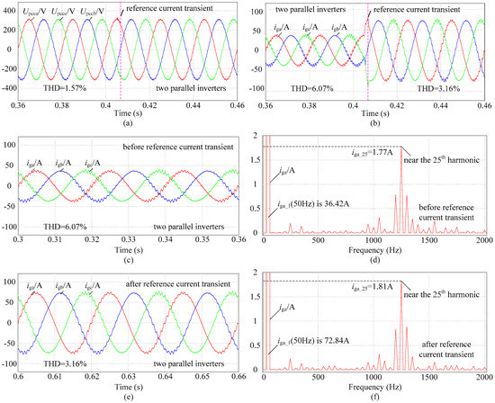
Figure 12.
Simulation waveforms of point of common coupling (PCC) voltage uPCC and grid-connected current ig in case I during reference current transient (two parallel inverters). (a) PCC voltage uPCC; (b) grid-connected current ig; (c) grid-connected current ig (before); (d) spectrogram of grid-connected current ig (before); (e) grid-connected current ig (after); (f) spectrogram of grid-connected current ig (after).
In case II, the transient simulation waveforms of PCC voltage uPCC and the grid-connected current ig are depicted in Figure 13a,b. From Figure 13a, the distortion rate of PCC voltage uPCC is 0.82%. The grid-connected current ig and corresponding spectrum before the reference current surges are shown in Figure 13c,d. The distortion rate of the grid-connected current ig is 3.27%, the resonance point is near the 39th harmonic (1950 Hz), and the resonance peak is 0.88 A. The grid-connected current ig and corresponding spectrum after the reference current suddenly increases are shown in Figure 13e,f. The distortion rate of the grid-connected current ig decreases to 1.51%, the resonance point is still near the 39th harmonic (1950 Hz), and the resonance peak value is 0.79 A. Meanwhile, the power quality of the grid-connected current can be significantly improved, and the resonance phenomenon has obviously decreased.
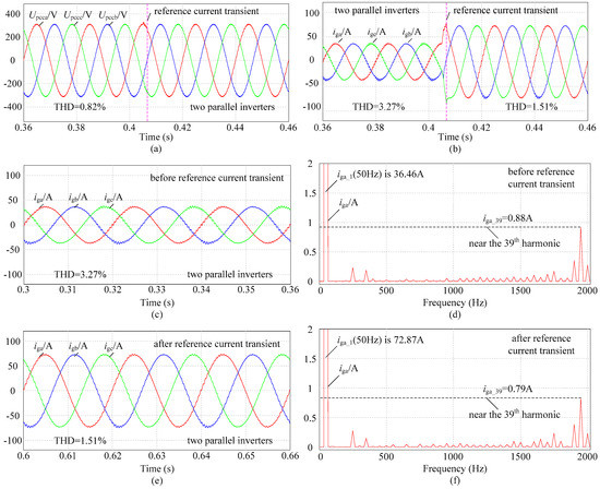
Figure 13.
Simulation waveforms of PCC voltage uPCC and the grid-connected current ig in case II during reference current transient (two parallel inverters). (a) PCC voltage uPCC; (b) grid-connected current ig; (c) grid-connected current ig (before); (d) spectrogram of grid-connected current ig (before); (e) grid-connected current ig (after); (f) spectrogram of grid-connected current ig (after).
When seven inverters are connected to a weak grid in cases I and II, the RMS of reference grid-side inductor current irefm for each grid-connected inverter is 10.71 A. Therefore, the RMS of the reference grid-connected current igref is 75 A for seven parallel inverters. The simulation waveforms and spectrograms of PCC voltage uPCC and the grid-connected current ig are shown in Figure 14 and Figure 15. The simulation results of the grid-connected current with seven parallel inverters are shown in Table 4. In case I, the system is in an unstable state. The resonance phenomenon is obvious. The reason is that the high-frequency harmonic current frequency is equal to or close to the parallel resonance frequency of self-impedance, resulting in a parallel resonance or quasi-resonance of the impedance network. The grid-connected current is still severely polluted by the impedance coupling interactions between the inverters and the grid. In case II, the distortion rate of the grid-connected current ig is 3.38%, the resonance point is near the 39th harmonic (1950 Hz), and the resonance peak is 1.51 A. Due to the sufficient resistive damping introduced to the impedance network, the system can operate stably. Therefore, case II can effectively improve the power quality of the grid-connected current and suppress the oscillation of the paralleled multi-inverter system.
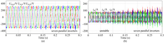
Figure 14.
Simulation waveforms of PCC voltage uPCC and the grid-connected current ig in case I (seven parallel inverters). (a) PCC voltage uPCC; (b) grid-connected current ig.
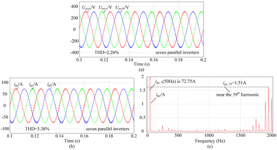
Figure 15.
Simulation waveforms of PCC voltage uPCC and the grid-connected current ig in case II (seven parallel inverters). (a) PCC voltage uPCC; (b) grid-connected current ig; (c) spectrogram of grid-connected current ig.
Table 4.
Simulation results of grid-connected current with seven parallel inverters.
6. Experimental Verification
To verify the validity of simulation analysis, a hardware-in-the-loop experimental platform based on a real controller TMS320F2812 digital signal processor (DSP) (Texas Instruments, Inc, Dallas, TX, USA) and a real-time laboratory (RT-LAB) (Opal-RT Technologies, Montreal, QC, Canada) was built [26], as shown in Figure 16a. The system parameters are shown in Table 2. The hardware-in-the-loop experimental platform mainly includes an RT-LAB simulator OP5700 (Opal-RT Technologies, Montreal, QC, Canada), real controllers of grid-connected inverters, a host computer as a real-time control interface, and an oscilloscope, as shown in Figure 16b. The main circuit model of the system was established in the host computer, which was loaded to the OP5700. When the model was running, the OP5700 sent the analog signals (voltages and currents) to the real controllers through the input/output (I/O) ports in real time. After data processing, the real controllers transmitted the digital control signals (pulses) to OP5700 through the I/O ports in real time. The data interacted in real time during the simulation process to ensure the normal operation of the system. The measurement information during the simulation were converted into analog signals through the I/O ports, which could be observed on the oscilloscope.
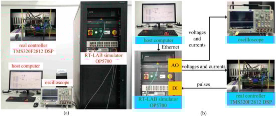
Figure 16.
Experimental platform for paralleled multi-inverter system based on hardware-in-loop simulation. (a) Whole; (b) Structure.
When two inverters operated in parallel, as in case I and case II, the RMS values of reference for the grid-side inductor current irefm for each grid-connected inverter increased from 18.75 A to 37.5 A at 0.405 s. Therefore, the RMS of reference grid-connected current igref increased from 37.5 A to 75 A for two parallel inverters. The transient experimental waveforms and spectrograms in case I and case II are depicted in Figure 17 and Figure 18. Experimental results of the grid-connected current with two parallel inverters are shown in Table 5. Before the reference current surged in Figure 17b, the distortion rate of the grid-connected current ig was 7.01%, the resonance point was near the 25th harmonic (1250 Hz), and the resonance peak was 2.66 A. After the reference current suddenly increased in Figure 17c, the distortion rate of the grid-connected current ig decreased to 4.22%, the resonance point was still near the 25th harmonic (1250 Hz), and the resonance peak value was 2.89 A. Thus, the grid-connected current apparently contained high-frequency ripples, and it is obvious that the major harmonics are 25th harmonics.
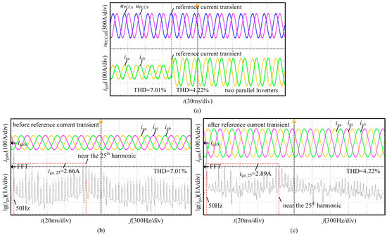
Figure 17.
Experimental waveforms of PCC voltage uPCC and grid-connected current ig in case I during reference current transient (two parallel inverters). (a) PCC voltage uPCC and grid-connected current ig; (b) grid-connected current ig and spectrogram (before); (c) grid-connected current ig and spectrogram (after).
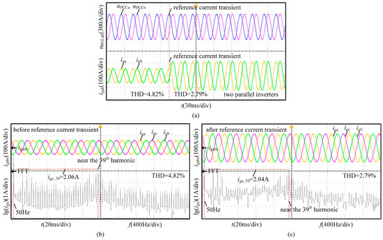
Figure 18.
Experimental waveforms of PCC voltage uPCC and grid-connected current ig in case II during reference current transient (two parallel inverters). (a) PCC voltage uPCC and grid-connected current ig; (b) grid-connected current ig and spectrogram (before); (c) grid-connected current ig and spectrogram (after).
Table 5.
Experimental results of the grid-connected current with two parallel inverters.
Before the reference current surged in Figure 18b, the distortion rate of the grid-connected current ig was 4.82%, the resonance point was near the 39th harmonic (1950 Hz), and the resonance peak was 2.06 A. After the reference current suddenly increased in Figure 18c, the distortion rate of grid-connected current ig decreased to 2.79%, the resonance point was still near the 39th harmonic (1950 Hz), and the resonance peak value was 2.04 A. Meanwhile, the power quality of grid-connected current can be significantly improved, and the resonance phenomenon has obviously decreased. Therefore, the distortion rate was smaller after the reference current surge in the same case. Moreover, before and after the reference current surged, the distortion rate in case II was less than case I.
When seven inverters operate in parallel in cases I and case II, the RMS of the reference grid-side inductor current irefm for each grid-connected inverter was 10.71 A. Therefore, the RMS of the reference grid-connected current igref was 75 A for the seven parallel inverters. The experimental waveforms and spectrograms in cases I and case II are shown in Figure 19 and Figure 20. The experimental results of the grid-connected current with the seven parallel inverters are shown in Table 6. As can be seen in Figure 19, the system is in an unstable state. The resonance phenomenon is obvious. The reason is that the high-frequency harmonic current frequency is equal to or close to the parallel resonance frequency of self-impedance, resulting in a parallel resonance or quasi-resonance of the impedance network. The grid-connected current is still severely polluted by the impedance coupling interactions between the inverters and the grid. From Figure 20, it can be seen that the distortion rate of the grid-connected current ig is 4.36%, the resonance point is near the 39th harmonic (1950 Hz), and the resonance peak is 2.99 A. Due to the sufficient resistive damping introduced to the impedance network, the system can operate stably. Therefore, case II can effectively improve the power quality of the grid-connected current and suppress the oscillation of the paralleled multi-inverter system.
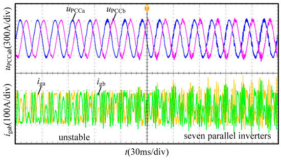
Figure 19.
Experimental waveforms of PCC voltage uPCC and the grid-connected current ig in case I (seven parallel inverters).
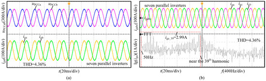
Figure 20.
Experimental waveforms of PCC voltage uPCC and the grid-connected current ig in case II (seven parallel inverters). (a) PCC voltage uPCC and grid-connected current ig; (b) grid-connected current ig and spectrogram.
Table 6.
Experimental results of the grid-connected current with seven parallel inverters.
7. Conclusions
In this paper, the oscillation suppression method by two notch filters is proposed to realize the virtual impedances and increase the whole system damping. The implementation form of the virtual impedances is presented by the proposed PCC voltage feedforward and grid-side inductor current feedback with two notch filters. The feedforward path of PCC voltage with the notch filter equals to a virtual impedance in parallel with inverter output impedance, which is designed to show low impedance at the harmonic oscillation frequency. By doing so, most high-frequency harmonic current will flow into the parallel virtual impedance branch, and it effectively suppresses the oscillation. Meanwhile, the feedback path of the grid-side inductor current with the notch filter is equivalent to a virtual impedance in series with inverter output impedance, which is designed to display low impedance at the fundamental frequency. This way, most of the fundamental frequency current flows into the grid branch with relatively low impedance. In addition, it improves the power quality of the grid-connected current. Finally, simulation and experimental results are provided to verify the validity of proposed control method.
Author Contributions
L.Y. and Y.C. provided the original idea for this paper. L.Y., H.W., A.L. and K.H. organized the manuscript and attended the discussions when analysis and verification were carried out. All the authors gave comments and suggestions on the writing and descriptions of the manuscript.
Funding
This research was supported by the National Key R&D Program of China under Grant No. 2017YFB0902000, and the Science and Technology Project of State Grid under Grant No. SGXJ0000KXJS1700841.
Conflicts of Interest
The authors declare no conflict of interest.
References
- Yu, Y.; Konstantinou, G.; Hredzak, B.; Agelidis, V.G. Power balance optimization of cascaded H-bridge multilevel converters for large-scale photovoltaic integration. IEEE Trans. Power Electron. 2016, 31, 1108–1120. [Google Scholar] [CrossRef]
- Guo, X.; Yang, Y.; Zhu, T. ESI: A novel three-phase inverter with leakage current attenuation for transformerless PV systems. IEEE Trans. Ind. Electron. 2018, 65, 2967–2974. [Google Scholar] [CrossRef]
- Bouloumpasis, I.; Vovos, P.; Georgakas, K.; Vovos, N.A. Current harmonics compensation in microgrids exploiting the power electronics interfaces of renewable energy sources. Energies 2015, 8, 2295–2311. [Google Scholar] [CrossRef]
- Hany, M.H. Whale optimisation algorithm for automatic generation control of interconnected modern power systems including renewable energy sources. IET Gener. Transm. Distrib. 2018, 12, 607–614. [Google Scholar]
- Li, X.; Fang, J.; Tang, Y.; Wu, X. Robust design of LCL filters for single-current-loop-controlled grid-connected power converters with unit PCC voltage feedforward. IEEE J. Emerg. Sel. Top. Power Electron. 2018, 6, 54–72. [Google Scholar] [CrossRef]
- Guo, X.; Yang, Y.; Wang, X. Advanced control of grid-connected current source converter under unbalanced grid voltage conditions. IEEE Trans. Ind. Electron. 2018, 65, 9225–9233. [Google Scholar] [CrossRef]
- Yang, Y.; Ye, Q.; Tung, L.J.; Greenleaf, M.; Li, H. Integrated size and energy management design of battery storage to enhance grid integration of large-scale PV power plants. IEEE Trans. Ind. Electron. 2018, 65, 394–402. [Google Scholar] [CrossRef]
- Rohner, S.; Bernet, S.; Hiller, M.; Sommer, R. Modulation, losses, and semiconductor requirements of modular multilevel converters. IEEE Trans. Ind. Electron. 2010, 57, 2633–2642. [Google Scholar] [CrossRef]
- Remon, D.; Cantarellas, A.M.; Mauricio, J.M.; Rodriguez, P. Power system stability analysis under increasing penetration of photovoltaic power plants with synchronous power controllers. IET Renew. Power Gener. 2017, 11, 733–741. [Google Scholar] [CrossRef]
- Malinowski, M.; Gopakumar, K.; Rodriguez, J.; Perez, M.A. A survey on cascaded multilevel inverters. IEEE Trans. Ind. Electron. 2010, 57, 2197–2206. [Google Scholar] [CrossRef]
- Amin, M.; Molinas, M. Small-signal stability assessment of power electronics based power systems: A discussion of impedance- and eigenvalue-based methods. IEEE Trans. Ind. Appl. 2017, 53, 5014–5030. [Google Scholar] [CrossRef]
- Bakhshizadeh, M.K.; Yoon, C.; Hjerrild, J.; Bak, C.L.; Kocewiak, Ł.H.; Blaabjerg, F.; Hesselbæk, B. The application of vector fitting to eigenvalue-based harmonic stability analysis. IEEE J. Emerg. Sel. Top. Power Electron. 2017, 5, 1487–1498. [Google Scholar] [CrossRef]
- Sun, J. Impedance-based stability criterion for grid-connected inverters. IEEE Trans. Power Electron. 2011, 26, 3075–3078. [Google Scholar] [CrossRef]
- Yang, L.; Chen, Y.; Luo, A.; Chen, Z.; Zhou, L.; Zhou, X.; Wu, W.; Tan, W.; Guerrero, J.M. Effect of phase-locked loop on small-signal perturbation modelling and stability analysis for three-phase LCL-type inverter connected to weak grid. IET Renew. Power Gener. 2008. [Google Scholar] [CrossRef]
- Xu, J.; Xie, S.; Tang, T. Improved control strategy with grid-voltage feedforward for LCL-filter-based inverter connected to weak grid. IET Power Electron. 2014, 7, 2660–2671. [Google Scholar] [CrossRef]
- Harnefors, L. Modeling of three-phase dynamic systems using complex transfer functions and transfer matrices. IEEE Trans. Ind. Electron. 2007, 54, 2239–2248. [Google Scholar] [CrossRef]
- Wang, X.; Blaabjerg, F.; Liserre, M.; Chen, Z.; He, J.; Li, Y. An Active Damper for Stabilizing Power-Electronics-Based AC Systems. IEEE Trans. Power Electron. 2014, 29, 3318–3329. [Google Scholar] [CrossRef]
- Yang, D.; Ruan, X.; Wu, H. A real-time computation method with dual sampling modes to improve the current control performances of the LCL-type grid-connected inverter. IEEE Trans. Ind. Electron. 2015, 62, 4563–4572. [Google Scholar] [CrossRef]
- Li, X.; Wu, X.; Geng, Y.; Yuan, X.; Xia, C.; Zhang, X. Wide damping region for LCL-type grid-connected inverter with an improved capacitor-current-feedback method. IEEE Trans. Power Electron. 2015, 30, 5247–5259. [Google Scholar] [CrossRef]
- Dannehl, J.; Fuchs, F.W.; Hansen, S.; Thogersen, P.B. Investigation of active damping approaches for PI-based current control of grid-connected pulse width modulation inverters with LCL filters. IEEE Trans. Ind. Appl. 2010, 46, 1509–1517. [Google Scholar] [CrossRef]
- Komurcugil, H.; Altin, N.; Ozdemir, S.; Sefa, I. Lyapunov-function and proportional-resonant-based control strategy for single-phase grid-connected VSI with LCL filter. IEEE Trans. Ind. Electron. 2016, 63, 2838–2849. [Google Scholar] [CrossRef]
- Chen, Z.; Chen, Y.; Guerrero, J.M.; Kuang, H.; Huang, Y.; Zhou, L.; Luo, A. Generalized coupling resonance modeling, analysis, and active damping of multi-parallel inverters in microgrid operating in grid-connected mode. J. Mod. Power Syst. Clean Energy 2016, 4, 63–75. [Google Scholar] [CrossRef]
- He, J.; Li, Y.; Bosnjak, D.; Harris, B. Investigation and active damping of multiple resonances in a parallel-inverter-based microgrid. IEEE Trans. Power Electron. 2013, 28, 234–246. [Google Scholar] [CrossRef]
- Zheng, C.; Zhou, L.; Xie, B.; Zhang, Q.; Li, H. A stabilizer for suppressing harmonic resonance in multi-parallel inverter system. In Proceedings of the IEEE Transportation Electrification Conference and Expo, (ITEC Asia-Pacific), Harbin, China, 1–6 August 2017. [Google Scholar]
- Jeong, S.-G.; Park, M.-H. The analysis and compensation of dead-time effects in PWM inverters. IEEE Trans. Ind. Electron. 1991, 38, 108–114. [Google Scholar] [CrossRef]
- Shuai, Z.; Huang, W.; Shen, C.; Ge, J.; Shen, Z.J. Characteristics and restraining method of fast transient inrush fault currents in synchronverters. IEEE Trans. Ind. Electron. 2017, 64, 7487–7497. [Google Scholar] [CrossRef]
© 2018 by the authors. Licensee MDPI, Basel, Switzerland. This article is an open access article distributed under the terms and conditions of the Creative Commons Attribution (CC BY) license (http://creativecommons.org/licenses/by/4.0/).