1. Introduction
The traditional grid has been criticized due to the one way of communication flow (top-bottom) and therefore is unable to response quickly to emergency events. The targeted grid attacks, unplanned contingencies or natural disaster phenomenon may pose a significant risk of power grid failures, which may subsequently cause partial or complete electricity blackouts. Long-term electricity blackouts without restorations do not only cause huge disruptions within communities but also may significantly reduce the economic and social welfare. For this reason, the smart grid concept brings into the action in order to compensate such shortcomings. Through the integration of information and communication technology (ICT) in the smart grid, this allows the prompt bi-directional communication flow within the electrical grid [
1,
2]. Such mechanism speeds up the energy trading, response and recovery purpose as before the communication may have broken down completely (assuming standby generations are available to power up the communication system for a short time period) after a disaster outbreak. This prevents the need to rely on the irreversible top-bottom communication flow, which is slow and ineffective in responding to unplanned contingencies (as the communication system may have already failed before reaching to the bottom level).
A microgrid, on the other hand, is an integrated low-voltage (LV) power delivery system in the smart grid composed of loads, a distributed energy resource (DER) such as a standby generator (non-renewable energy source), a renewable energy source (RES) and an energy storage system (ESS) operating as a single controllable load connected to the main grid [
1,
3]. The microgrid has the ability to isolate its LV grid portion from the main grid (grid-connected) or the partial isolation (islanding) within the LV network, in the case of outage/contingency events [
1].
There are two types of microgrid controls within the smart grid network: centralized and decentralized control. According to Vaccaro et al. [
4] and Olivares et al. [
5], a core microgrid controller in the centralized control provides appropriate control actions (set points) to the local controllers of different DER units and loads that optimizes the local energy production and the main grid. A decentralized control, on the other hand, allows the full autonomy for all local units, where units are ‘smart’ and can communicate with each other to form a larger topology. In present, both control mechanisms have their drawbacks. According to Vaccaro et al. [
4] and Olivares et al. [
5], a fully centralized control is infeasible to be deployed in geographically sparse areas, where extensive communication infrastructure and computations are required. On the other hand, a fully decentralized approach is not possible due to strong coupling points within units and localised information. Hence, the system will not be aware the overall system operation and the control actions from the microgrid controller. As asserted by Hatziargyriou et al. [
6] and Erol-Kantarci et al. [
1] and the main finding by Winkler et al. [
7], the presence of generation in proximity of the demand is critical to enhance the overall power reliability and quality. As holistic information of the grid is required in responding to adverse events, a centralized microgrid control is considered in this paper.
The energy management system of microgrid is based on the localised controllable DER and loads with the combination of the Unit Commitment (UC) and Optimal Power Flow (OPF) models [
8,
9]. The main aim of the microgrid is to optimally allocate the DER that will minimize the monetary cost and increase the performance of grid operations. Elsied et al. [
8] proposed an advanced real-time energy management system for the microgrid in order to achieve the optimal allocation of DER. The optimization model consisted of a generalized economic cost as the objective function with operational constraints and the problem was solved using the Binary Particle Swarm optimization (PSO) algorithm. Meanwhile, Shi et al. [
10] proposed a centralized-based distributed energy management system where the microgrid central controller and the local controllers were joined to compute an optimal schedule. The system applied complex optimal power flow as the problem formulation. Parisio et al. [
11] presented a Model Predictive Control (MPC) with Mixed Integer Linear Programming (MILP) framework which included the UC, economic dispatch and ESS for grid interaction and curtailment schedule in an experimental microgrid located in Athens. Hossienzadeh and Salmasi [
12] proposed a robust optimal power management system for an isolated AC/DC microgrid, where the system performance was assessed through MILP-based minimization of the cost function with operational constraints. The system also considered the uncertainties in the power output and forecast generation errors, and two-level-based control mechanism of charging/discharging storage batteries. A smart energy management system to optimize the operation of microgrid was presented by Chen et al. [
13] where the optimization problem of ESS, economic load dispatch and the optimization of DER was simplified into a single-objective problem. Yang et al. [
14] proposed a novel stochastic optimal control strategy focusing in independent microgrids based on the integration of ESSs and traditional synchronous generators. The approach was based on an improved design of linear quadratic Gaussian controller and the consideration of the ESS’s current state of charge (SOC) that prevented the batteries’ overcharging and overdischarging problems, thus adaptively regulating the power output to minimize the frequency fluctuations. Wang et al. [
15] proposed a hierarchical three-level multi-agent system (distribution network, microgrid and distributed generation level) and decentralized technique for optimal coordination and operation of several AC/DC hybrid microgrids. At the microgrid level, the MILP was performed in an individual microgrid and a consensus algorithm was further utilized to optimally coordinate multiple microgrids. Interestingly, a fuzzy logic-based artificial neural network power management system was proposed by Chettibi et al. [
16] to minimize the energy purchased from the electrical grid through maximum untilization of RES and ESS subject to variable conditions such as climate, demand and disturbance in electrical grids.
Overall, the intensive concentration in optimal allocation of DER is the main target that reduces the microgrid operation cost, and increases the stability and performance. However, less attention has been paid to microgrid approaches in the grid resilience subject to adverse events, as well as the quantification of grid resilience. The enhanced performance and economical operation cost may not reflect the desired grid resiliency. As indicated by Panteli and Pierluigi [
17], the cost-efficient solution might indicate the extra investment of smart technologies, but the degree of robustness of the investment might be uncertain. Therefore, conceptualising the concept of resilience in power grids may help in balancing the monetary costs and resilience.
According to Panteli and Pierluigi [
17], Cano-Andrade et al. [
18], Bollinger [
19], Khodaei [
20] and Liu et al. [
21], resilience is the ability of a power system to withstand/remain in a state during a failure in an efficient manner, and to quickly restore to the normal operating state. A generic resilience framework ‘4Rs’—robustness, redundancy, resourcefulness, and rapidity—was developed by the Multidisciplinary and National Center for Earthquake Engineering Research to be applicable for critical infrastructures [
17]. Four resilience indices are introduced by Liu et al. [
21], which are the number of line outages, loss of load probability (LOLP), expected demand that cannot be supplied, and the difficulty of grid recovery indexes. However, resilience assessments as introduced by Liu et al. [
21] contradicted with the resilience computation by Cano-Andrade et al. [
18], Bollinger [
19], as the grid resilience in this case is determined by the extent in which the amount of energy demand within consumers are met when there is a disturbance in the grid.
Several resilience-based power system operations have been considered to address the disaster and contingency events. Romero et al. [
22] applied stochastic programming to optimize the capacity enhancement strategies of the transmission and generation that increased the resilience of large-scale power systems against seismic risks (earthquakes). Winkler et al. [
7] presented a new methodology combining the hurricane damage predictions and different grid topological assessments to characterise the impact of hurricanes towards the reliability of the power grid. The analysis concluded that the ring-meshed grid topology provided superior performance during hurricane hazards due to the presence of a centralized substation ring. Ouyang and Dueñas-Osorio [
23] introduced the time-dependent resilience assessment of urban infrastructure systems. A resilience-oriented microgrid optimal scheduling model was proposed by Khodaei [
20] that minimized the reduction in microgrid load by efficiently scheduling the available resources at a point of supply interruption from the main grid. A holistic framework for optimal microgrid operation to guarantee uninterrupted power supply to critical loads was proposed by Detroja [
24]. The framework consisted of three optimization modules to perform the load scheduling, UC and power balancing. Bahramirad [
25] presented the economic and emergency operation of ESS in a microgrid, by introducing outages within generation units and transmission lines. Erol-Kantarci et al. [
1] focused on clustering methods that multiple smart microgrids (SMGs) would operate collaboratively to form a smart microgrid network (SMGN) of a ring topology. The main aims are to accelerate the deployment of low-carbon energy resources and to ensure the survivability of the SMGN through resource sharing within smart grid networks. The approach, however, neglected the cost function and the grid resilience. The full utilization of low carbon energy resources may not guarantee the low operational cost and the grid resilience.
However, the lack of time-dependent resilience quantification and assessment impede the justification of microgrid penetrations in enhancing grid resilience. Still, the resilience concept was only briefly introduced in the context. Ouyang and Dueñas-Osorio [
23] asserted that the time-dependent resilience analysis enabled the evolvement in the power grid, the process improvements and the possibility of grid underperformance issues. Additionally, resilience assessments were particularly being focused within large scale applications of generation, transmission and the bulk grid in the sparsely populated area.
In this regard, this paper aims to model a holistic grid distribution network composing the MV (mid-voltage) and LV (low voltage) level of an urban grid. The model further mitigates the impact of supply failure during disasters and emergency responses, especially in the critical infrastructures that are highly dependent on the availability of electricity. The contributions of the proposed method are as follows:
- (i)
The proposed model is a novel approach that creates a new methodology to specifically illustrate the time-dependent-based grid resilience during the grid recovery process for an outage event;
- (ii)
The modelled system enables utility planners or engineers to foresee the grid structure that is vulnerable to outages (partial or complete), as well as generation intermittencies and failures;
- (iii)
The simulated model allows the most economical approach of meeting demand shortage towards critical infrastructures while maintaining the grid resilience;
- (iv)
The possibility of an overloaded electrical grid can be prevented and thus defers the need for network reinforcements.
The paper is organised as follows:
Section 2 describes the system model for the grid architecture.
Section 3 describes the formulation problem and the proposed solution of the optimization problem, the modelling of ESS and the resilience calculation.
Section 4 presents the model simulation settings prior the simulation.
Section 5 demonstrates case studies of an urban grid for normal and outage operation.
Section 6 provides conclusions.
2. System Model
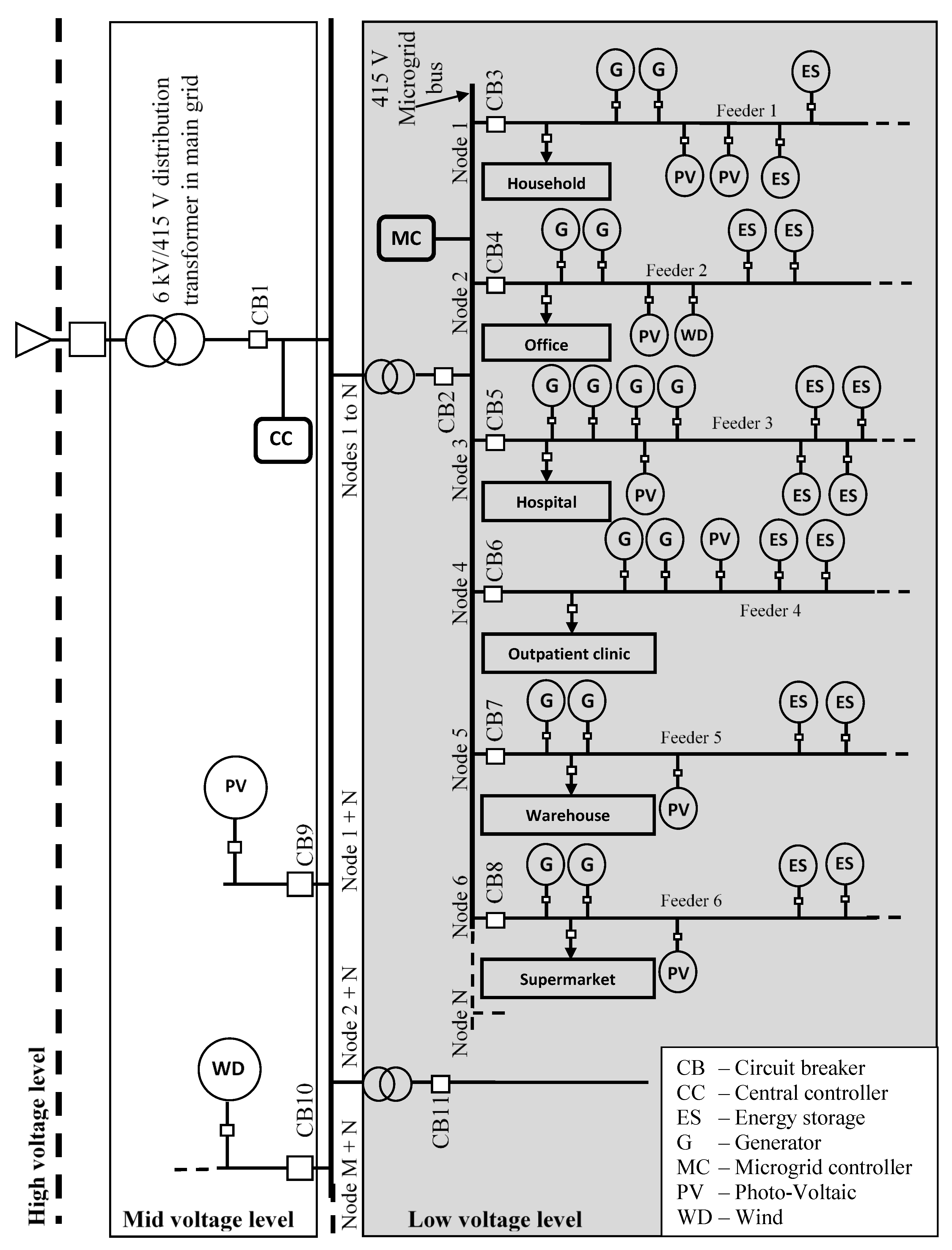
A common microgrid configuration is presented in
Figure 1. Each node (Node 1, Node 2, ⋯, Node
) includes the component of MV and LV which includes the generator (in the MV level), electrical loads for the end consumers, and small scale diesel-powered standby generators, ESS and RES that are connected via electrical interconnectors for the LV level. Both
M and
N denote the number of nodes for the MV and LV level correspondingly. The feeders transfer the power from generators to the end consumers [
26]. The microgrid is connected to the MV grid through a transmission line. A circuit breaker (CB),
, is installed that acts as the protection mechanism to connect or disconnect the MV grid from the high level grid. Similarly,
is used to protect the LV microgrid from the MV grid.
The grid can have two operation modes: normal and islanded state. In normal state, the microgrid is interacted with the MV grid. On the contrary, during an outage event, the microgrid can operate in an islanded mode by opening
in
Figure 1. This is to enable the continuous supply of energy within the LV microgrid without interruptions. The microgrid controller will send control actions to standby generator and ESS to provide energy to the microgrid. Similarly, the MV grid can still operate through on-site ‘self-generation’ by opening
. In addition, an islanded operation can also occur within a linked connection in the microgrid. For example, all the components in Node 3 of the microgrid can operate in islanded mode if
is opened. The remaining nodes operate normally and interact with the MV grid.
It is assumed in this case that the microgrid controller has the capability to perform switching by isolating the LV network from the grid entirely due to the sophisticated design and capability of CBs. This is because there is an electronic control applied at the gateway controller, which is relevant to the protection and reliability operation schemes during a contingency and when switching from high voltage generation to MV–LV generation. However, it is not the scope of this paper to study the switching, protection and dynamic operation performance. Additionally, during an outage event, we assumed that the electricity line connections within the islanded node (the connection between a DER and a critical infrastructure) would have robust design features where energy is delivered without suffering significant energy losses, regardless of the location. Henceforth, choices of the geographical location and the robust design features of electricity connections would not affect the microgrid operation in this case.
The system model in this paper concentrates on the centralized perspective of the microgrid controller in optimizing the localised energy productions. This is achieved by performing an energy balancing optimization based on a cost minimization function of the DER such as standby generator, ESS and RES. Through the energy balancing optimization algorithm, the model automatically identifies the most economical approach of meeting the demand shortage within critical infrastructures while maintaining the grid resilience.
3. Problem Formulation
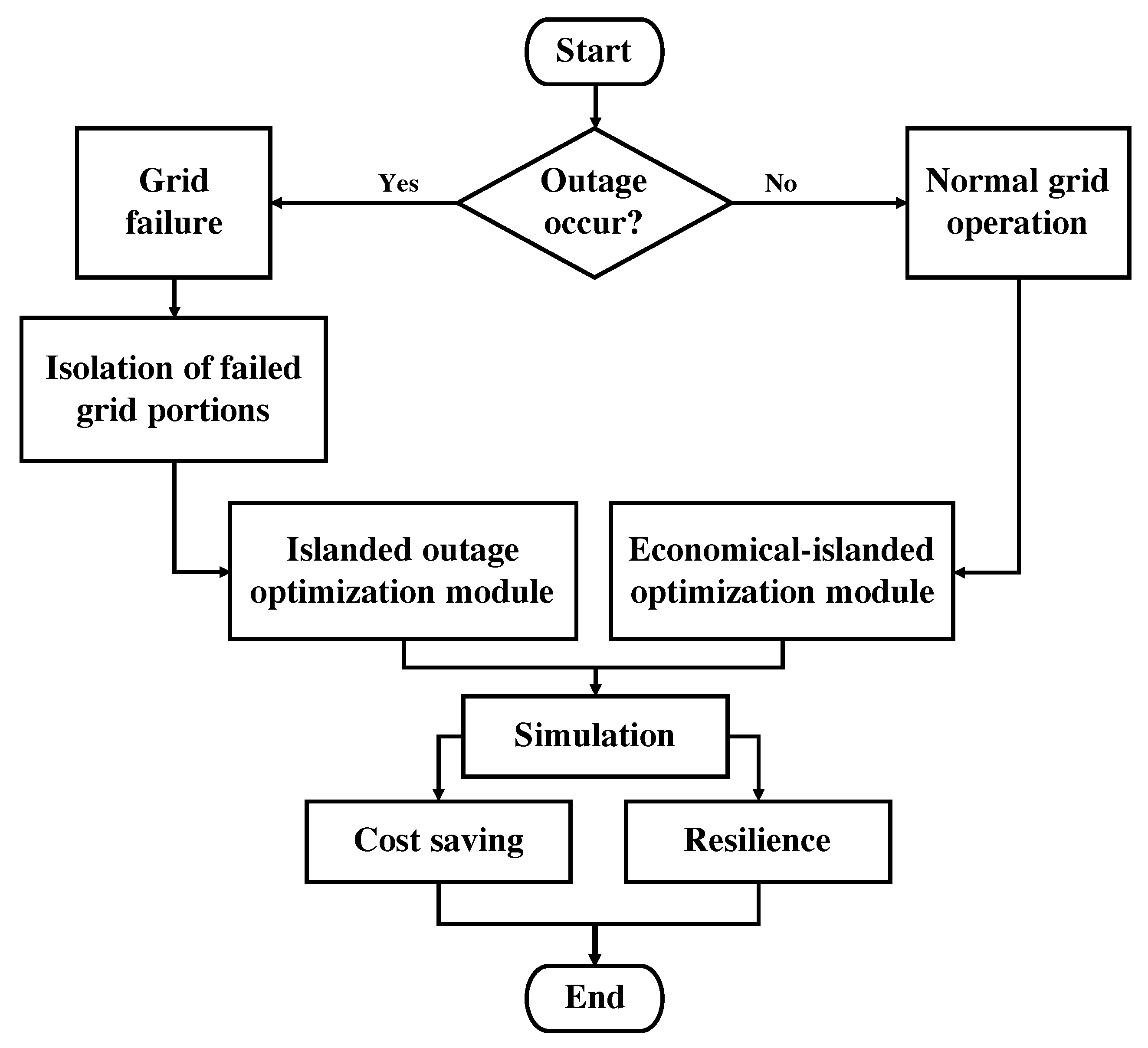
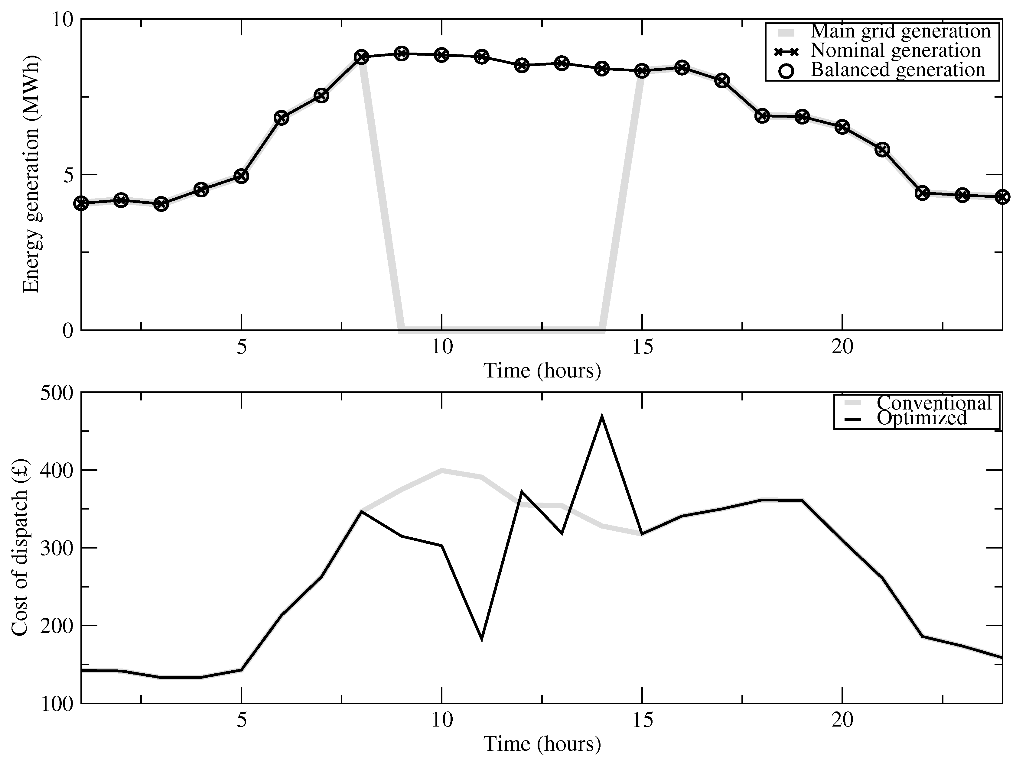
As before with proceeding to the problem formulation of the grid optimization, a flow chart illustrating the integration process of the proposed grid optimization module that optimises the monetary costs and maintaining the grid resilience is demonstrated in
Figure 2. The process begins with the determination of the current grid operation state. If no outage occurs, the grid operates in normal mode and the so-called ‘economic-based’ islanding operation is introduced to prevent the LV level grid from drawing the electricity from the main grid at times of high electricity price. This allows the optimal cost operation between the MV/LV level grid in responding to the market price. In contrast, if outage occurs, the portion of electrical grid with outage is isolated from the remaining grid portion and the specialized islanded grid optimization module is used to find the optimal operational cost of dispatching generating units in responding to sudden demand shortage due to an outage. For both grid operational modes, the performance of optimizations is evaluated through cost savings and resilience analysis.
3.1. Grid Optimization Problem
The optimization problem is typically the economic dispatch in the combination of the UC problem. The economic dispatch optimizes the most economical way of dispatching generating units (except RES) while meeting the nationwide demand. Due to the nature of generation intermittency within RES, the generation output shortages within RES are balanced by available standby generators, mid-scale power plant and ESS. Hence, there is no associated optimization performed in RES in this case. Lau et al. [
27] provide detailed fuel consumption and cost function in the economic dispatch problem. In contrast, the UC problem deals with coordinations of committable and non-committable state of standby generators, as well as the varied loads, based on hourly (h) intervals of scheduling slots.
The optimization problem formulations from Bahramirad [
25], Zendehdel et al. [
28], Hedman et al. [
29], Khodaei [
30], Howlader et al. [
31] are followed. A single objective function optimization problem is proposed in this paper, with the combination of economic dispatch and UC problems. This is to reduce the complexity and prevent the arising of multi-objective optimization problems [
32]. The objective function, as well as constraints, are formulated based on the linear programming (LP) problem. This is to prevent the arising of nonlinear problems. In fact, a constrained linear programming is a convex optimization problem that has an extreme point of the feasible set, and thus will have an optimal solution. Since the adaptive and better quality of decision is peculiarly critical in an emergency situation; therefore, LP optimization problem is highly recommended [
33]. The model also presumes that the microgrid has more energy generation than loads for all nodes in the microgrid and no load curtailment for the node, or for the loads that are implemented in this case.
3.2. Objective Function for Normal Operation
The objective function for normal operation (
) as formulated in Equation (
1) is based on three important terms, where the first term is the operating cost of the dispatched units, the second term deals with ESS and the final term deals with the cost of the electricity purchased from the main grid (high level):
The g, s and t index the corresponding generating units (diesel-powered standby generation units), ESS and the time period. and denote the standby generators, ESS and the time period. is the transmission line power. is the energy dispatch of corresponding unit g. is the start-up cost. is the energy generated in s at time t. is the shutdown cost. is the electricity market price at the time where there exists electricity connection from the LV to MV level. is the commitment state binary value of unit g.
Ever since the wholesale electricity market liberalization in early 1990s, the wholesale electricity market has become a very fundamental parameter to balance the acceptable costs for consumers’ demand, security of supply and the fulfilment of environmental policy from the national to global level [
34,
35]. Weron [
34] provided a very useful guideline on the electricity market trading process that involved typically a day-ahead auction market, where interested parties submit their bids and offers for the delivery of electricity based on their availability of generation capacity for the next day as before the trading market is closed. There are a variety of methods and ideas adopted for optimal electricity price forecasting. However, it is not the scope of this paper to forecast the day-ahead electricity price. Instead, for simplicity purposes, the electrical exchange data will be obtained from a public domain.
In Equation (
1), the first term refers to the generation cost that is denoted by
. For thermal units, the generation cost is presented in a quadratic function and is simply approximated by a piecewise linear approximation. The generator’s committable state is represented by the variable
.
equals one when the unit is committable and zero when the unit is not committable. Hence, there will be a generation cost when the commitment state of the unit is one and, in contrast, zero generation cost when the unit is not committed. The
and
of thermal units are also modelled explicitly. The
variable is introduced as
and, in contrast, the
variable as
. Both
and
are binary variables. When unit
g is switched on at current time
t but has been switched off until
, the
is imposed with
= 1. Otherwise,
= 0. Similarly, when
g is switched off at time
t but has been switched on until
, the
cost will be imposed with
= 1 and, otherwise,
= 0. The relationship of
and
with the UC variable
can be presented as:
For the second term, there is ESS cost when the energy is drawn from the main grid (ESS is in charging mode) at times of low electricity market prices . On the contrary, during the generation (discharging mode), zero generation cost is assumed to be imposed by ESS.
For the final term, depending on the operation state, there will be electricity costs when there is an interaction between the present and the main grid. In contrast, there will be zero electricity costs when no energy is drawn from the main grid.
The objective function as formulated in Equation (
1) optimizes
at every time step
t (e.g., current time
). The grid is further subject to the following operational constraints:
3.2.1. The Power Balance Constraint
The power balance constraint ensures that the total power generation from the LV and MV units would satisfy the overall load. It is defined as:
where
is total aggregated energy across the grid,
r indexes RES and
is the energy generated from RES.
,
and
are the total number of non-renewable generators, RES and ESS, respectively.
3.2.2. Unit Output Limit
The generation units are imposed by minimum and maximum amount of generation capacities:
where
is the minimum allowable capacity and
is the maximum allowable capacity of
at unit
g.
3.2.3. Ramp up and down Constraints
The ramp up and down rate is formulated as:
where
is the ramp up rate limit and
is the ramp down rate limit. The imposed ramping constraint limits the amount of a generating unit within two successive h. That is to say, a generator is not allowed to reach a maximum capacity due to the nature of operations [
27].
3.2.4. Transmission Line Capacity Constraint
The transmission line capacity limit between MV/LV level grid bus is formulated in Equation (
7). Equation (
8) formulates the distribution line limits within the LV level:
3.2.5. Spinning Reserve Requirement
The spinning (or operating) reserve is the additional required generating capacity and is made available to the electrical system operator within a short time interval to meet demand in case of contingency events such as generation or transmission failures, or sudden peak demands. The spinning reserve allows the responsive and speedy recovery of energy shortages (e.g., within 10 min) through fast acting generators that feed to the electrical grids. The spinning reserve requirement is formulated as:
The is the reserve requirement at time t. In this case, the spinning reserve is online but unloaded, which will be triggered by the central or the microgrid controller to commit if required. in this case is calculated as the percentage of the forecasted hly load.
3.2.6. Must Run and off Constraint
Generators are required to provide energy or to shutdown due to some operational circumstances:
The and indicates the gth unit that must run and off within the time interval, respectively.
3.3. Objective Function for Outage Operation
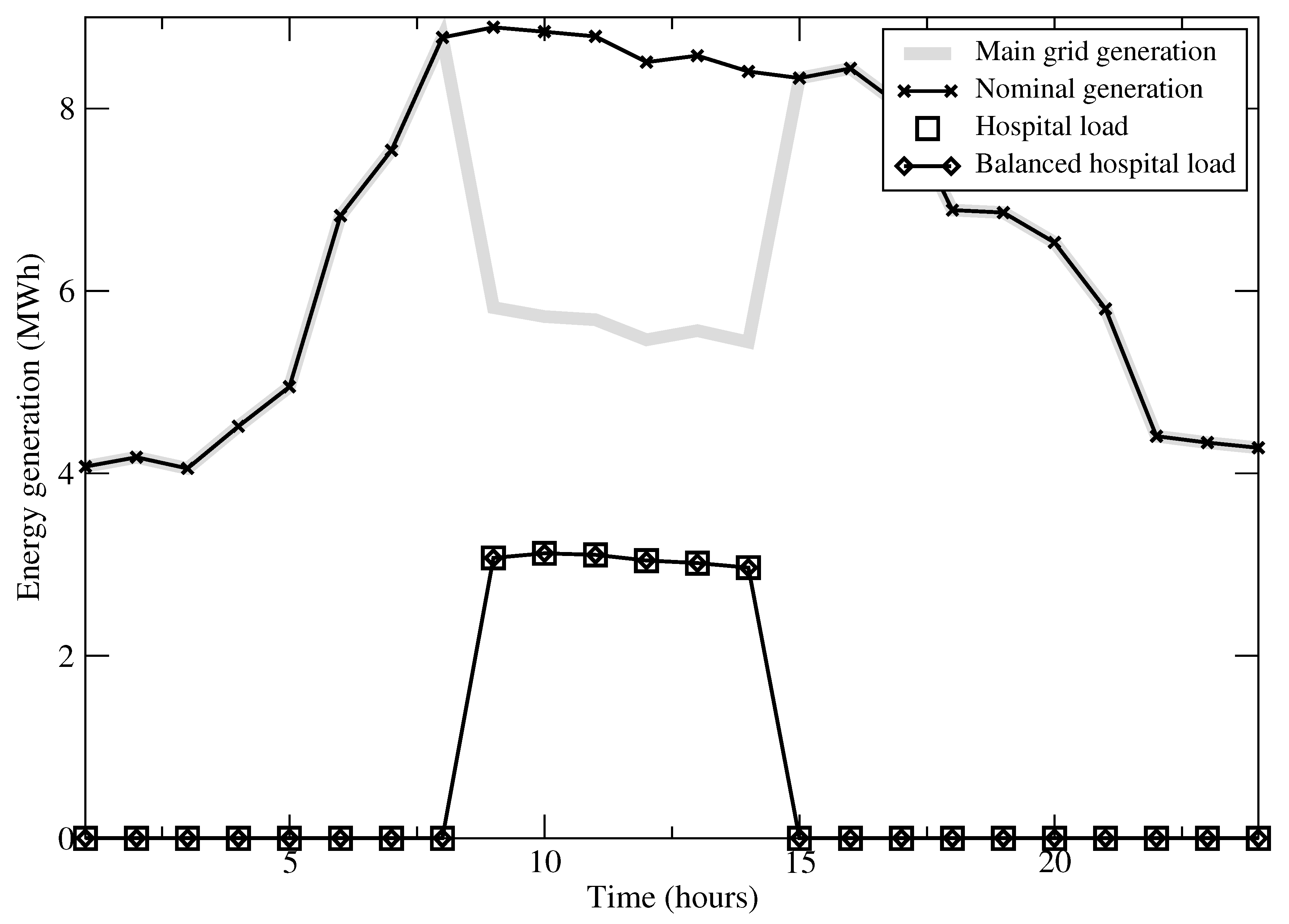
During an outage event, the objective is to supply the energy to critical loads from standby generators in economically efficient manner. The objective function for the outage operation
is similar to Equation (
1), but is intended only for contingency purposes:
The index i refers to the generating units in N-1 state and and is the total thermal generating units and ESS units in N-1 state: refers the N-1 contingency state of unit x at time t. is the N-1 state of ESS.
The operational control constraints are applied using Equations (
2) and (
4)–(
11). A
N-1 contingency criterion constraint is considered during an outage event. The
N-1 system compliance ensures the grid can survive any single outage in any links, and also the line across the MV/LV level grid. The generation and the transmission line output are constrained in the contingency situation:
The superscript
c denotes the contingency state. The
in Equation (
13) denotes the binary parameter for
N-1 contingency state of
x at time
t. The
when the generator is in contingency state and
for normal operations. If the
xth unit is not committable
, or the unit is in outage with
, the
xth unit generation output is zero. This is to indicate that an offline generator cannot respond during the contingency situation. Hence, the committable generating units are only allowed to operate in the contingency state. The operating constraints for committable generators during the contingency state will remain the same.
Similarly,
in Equation (
14) denotes the binary parameter for
N-1 contingency state of the transmission line between the MV and LV level. The
forces the transmission flows to be zero when the transmission line is in contingency state and otherwise,
for normal operations. Depending on the scale of damages, for example, if the transmission line is not affected, i.e.,
, the affected
xth generators in a node (
) will be in islanded mode of operation, whereas the unaffected area will be in normal operation mode.
The power balance equation in the contingency state is:
In order to continuously supply energy to critical infrastructure during the outage operation, the functionality of ESS is critical and therefore is modelled in the grid architecture.
3.4. ESS Model
ESS stores energy at times of low energy market prices (off-peak electricity demand), discharges the stored energy during high electricity market prices, low grid generation, and also the contingency situation in compensating the generation shortages. Methods of ESS operation and modelling by Bahramirad [
25], Howlader et al. [
31] are followed.
There are three important operating modes in ESS, which are the charging, discharging, and idle mode. For the contingency situation, the energy storage will discharge, based on the available storage capacity.
The energy stored in ESS is the state of charge (SOC). The SOC for ESS is formulated as:
is the SOC of ESS,
is the time interval in the SOC, and
s indexes ESS unit. The
in this case is denoted with positive and negative magnitude depending on the charge and discharge mode. From Equation (
16), during the charging mode, ESS is storing the energy, the
is negative and thus the value of
increases. On the contrary, during the discharging mode, ESS is said in generating the energy and the
is positive. Then, the value of
decreases. As clarified by Howlader et al. [
31], depending on the current storage technology, ESS is with the operating margin capacity of 80% upper limit and 20% lower limit:
In this case, it is assumed that the ESS is allowed to discharge the energy until ESS is partially exhausted (20%), and charge at 80% of the maximum capacity. Additionally, the instant charging/discharging capability is assumed as soon as a signal is sent by the microgrid controller. The charging and discharging mode of ESS is remained the same during a contingency event. However, the proportion of SOC may change and Equations (
16) and (
17) is modified as:
The operation of ESS is accomplished by adding the generation output to the energy balance equation (normal and outage operation) in Equations (
3) and (
15).
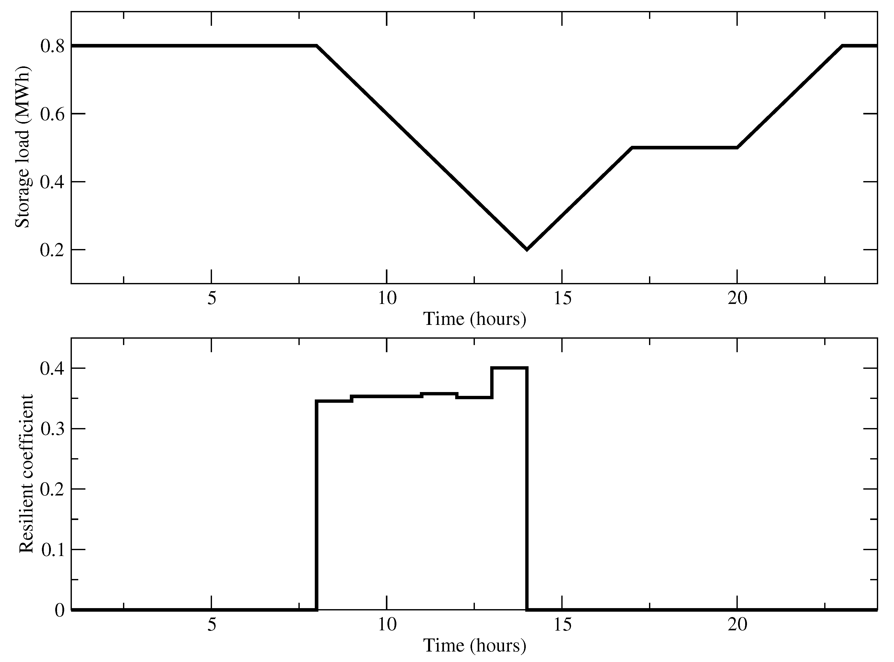
3.5. Resilience Metric
In order to access the resilience of a grid, a performance metric indicator is established. As in line with Cano-Andrade et al. [
18] and Bollinger [
19], the resilience metric in this paper is represented by the extent in which the amount of energy demand within consumers are met when there is a disturbance in the grid. The performance metric to calculate the resiliency is based on the fraction of demand served, or the amount of the energy produced by the microgrid during an outage [
18,
19]. The resilience coefficient in this case is therefore the fraction of demand served at
dth consumer (
) divided by the overall demand (
) in the contingency state:
4. Simulation Modelling and Settings
An IEEE 14-node test topology is used as the benchmark grid in this case. In order to perform a microgrid simulation in a IEEE test system, the original capacity of 280 MW in the test grid has been scaled down, such that each of the nodes can be configured as microgrid with the total 6.70 MW of the load capacity (≤10 MW). A random configuration of buildings consisting of eight blocks of offices, one large hospital, two outpatient clinics, three supermarkets, three warehouses blocks and 1000 residential houses has been simulated for a duration of one day. Samples of demand profiles are obtained from the portals (Elexon [
36], OpenEI [
37]). Outages of different durations are simulated (as illustrated in different grid operations). Contingency tests (Ejebe and Wollenberg [
38]) are performed by simulating single line failure in each case. The overall distribution of the generation and consumer loads in the grid architecture is modelled using the microgrid configuration in
Figure 1 and
Table 1. The distribution of load profile in this case is not intended to include the profiles of commercial services and domestic households within the same node. This is because most commercial services are connected with their own substations due to the huge amount of loads required.
Two types of RES—wind and solar-powered PV for LV and MV with 0.5 MW generating capacity of each are considered in this example, where the characteristic and generation profiles of RES are adopted from Jayaweera and Islam [
39] and Elexon [
40]. The generation data from Elexon [
40] is further rescaled to fit the current microgrid capacity. Four types of thermal units for microgrid which are non-renewable backup generators are considered in this example with 0.5–1.0 MW capacities, alongside with two mid-scale thermal (2.0 MW capacity each) for MV level grid. Specification of thermal units were originally adopted from Bahramirad [
25], Lau et al. [
27], with implemented modifications to fit the required generations to the load demands.
Two identical ESS units with a total of 2 MW storage capacity (1 MW each) are included in the simulation. Each ESS can be fully charged within 6 h in order to reach the maximum SOC of 9.6 MWh (within 20–80% of capacity).
The demand from each node is summed in order to provide the total aggregated demand across the grid (
). The timeline for the simulation is limited to 24 h with hly-based temporal resolution. As the time interval for the optimization is 1 h,
is applied in Equations (
16) and (
18).
The wholesale electricity market price data is obtained from the EPEX SPOT portal [
41,
42]. It is one of the UK’s power exchange providing the trading and clearing services for the wholesale market. EPEX SPOT portal provides historical data of the reference price data for the electricity. In this case, the 2017 year of reference price data is adopted, with additional calculation to compute the 24 h average whole electricity price data.
The optimization problems are solved using the MATLAB
® R2017b platform (version 9.3.0.713579, 64-bit, the MathWorks Inc., Natick, MA, USA) with 7th Generation Intel
® Core i5-7267U (3.1 GHz dual-core, 4 MB cache, up to 3.5 GHz) CPU and 8 GB (2133 MHz LPDDR3) of RAM. The simulations for optimization problems along with graphical illustration result plots are obtained for the duration of 0.8 s, thereby requiring minimal amount of computational efforts. The dual-simplex algorithm is applied for the LP problem, where the solution starts better than optimum but remains infeasible until the true optimum is reached along with feasible solution [
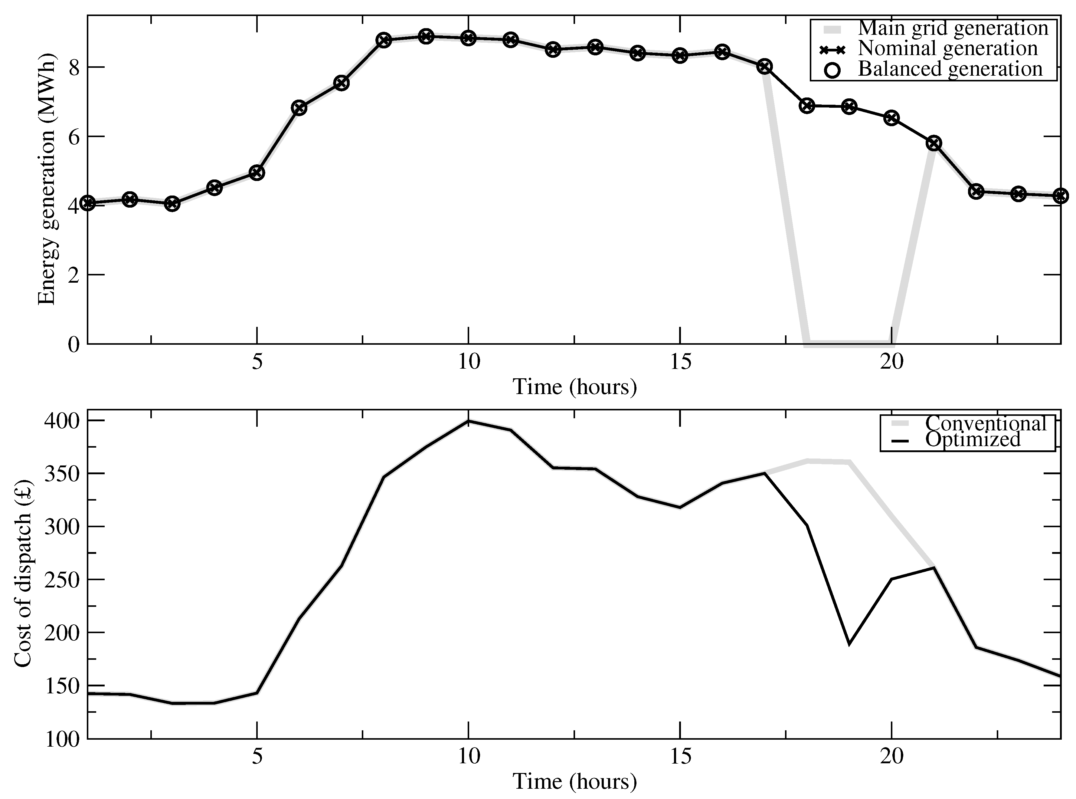
43]. The conventional operation of the grid is simulated with economic-based islanding in responding to the market price.
6. Conclusions
This paper proposes a resilient-based optimization module to balance the monetary costs and resilience. The outage with N-1 contingency criterion is applied by isolating the grid portions from the main load, depending on the scale of outages. The proposed model allows for the whole integration of the main grid supply, electricity connections, DER such as standby generators, ESS, RES, energy demand profiles and simulation of grid outages. The major breakthrough of this paper is the capability of performing the time-dependent resilience analysis of microgrid operation. The established resilience-optimization model represents a smart grid network that maintains the overall resilience across the grid subject to adverse events.
The involvement of ESS as well as RES in different scenarios is not only capable of providing contingency response but also has successfully mitigated the amount of generations produced by polluting standby generators, thus improving the environmental health.
The developed optimization model acts as the fundamental approach that can further support larger urban electricity grids with high flexibility. However, precautionary measures of microgrid penetrations should be performed in the future work to determine the marginal level of microgrid penetrations that will guarantee the grid safety and superior operations. As the current model concentrating on single line failure, a meshed grid topology for the model is essential not to only examine a single failure, but also to examine the multiple cascading failures across the grid. Future work should extend the capability of the proposed method. Additionally, as it is not the scope of this paper to compare different grid configurations, future work should consider the variety of grid configurations (for instance, baseline and the decarbonisation scenario) for performance evaluation purposes.


