How Reliable Are Standard Thermal Response Tests? An Assessment Based on Long-Term Thermal Response Tests Under Different Operational Conditions

Abstract

In this contribution, we analyze the results of a number of thermal response test (TRT) experiments performed during several years at the same location at our university campus in Valencia (Spain), a permeable saturated soil area with possible groundwater flow conditions. A combination of different heat injection rates, TRT operation times of up to 32 days, and various methods for parameter estimation of ground thermal properties have been applied to study their influence on the result and accuracy of TRTs. Our main objective has been to experimentally quantify the influence of groundwater flow heat advection using moving infinite and finite line-source theories, as well as to analyze the influence of factors such as test duration, sensor accuracy, and external thermal influences. We have shown that the traditionally used infinite and finite line-source models, as well as the moving line-source models, can accurately represent experimental temperature evolution, but that there are many caveats regarding the significance parameters extracted and its reproducibility and stability. These features can be improved if data from the first test days are disregarded for the analysis, obtaining a much faster convergence to the definitive soil parameter estimates, including the effective Péclet number that represents groundwater flow in our particular case.

1. Introduction

Shallow geothermal energy systems (SGES) are a solid alternative as a choice of system for heating [1,2], mixed heating, and cooling applications in buildings [3]. In comparison with other heating and cooling technologies, they offer plenty of advantages: Competitive levels of comfort, reduced noise levels, substantial savings of greenhouse gas emissions, and reasonable environmental safety. Their lower electrical consumption [4] and maintenance requirements lead to a competitive running cost [5] in such terms that SGES are recognized by the U.S. Environmental Protection Agency as being among the most efficient and comfortable heating and cooling systems available today [6].

The use of the in situ thermal response tests (TRT) to determine the thermal properties of the soil is a common practice for the design of air-conditioning systems based on ground coupled heat pumps. It is especially necessary in large-scale installations, where an erroneous calculation of the length of the borehole heat exchanger (BHE) will result in poor system performance if it is undersized, or unjustified extra costs if it is oversized. TRT in situ tests are widely used in industry and standardized today [7,8,9,10] and their basis is the comparison of the temperature response of a BHE to a constant heat injection or extraction, with the prediction of some simplified model of choice based on a few parameters to be fitted, including soil thermal conductivity. For reasons of simplicity and speed [11,12], among the widest used models [13], the basic reference is the Kelvin line-source theory, also termed the Infinite line-source (ILS) [14,15,16] model. Nevertheless, other approaches are becoming increasingly common, such as the finite line-source approach (FLS) [17,18,19], the cylinder-source model [14], commonly applied in Europe [11,20,21,22] and North America [23,24,25], or other models based on the use of capacitance and resistance analogs (like CaRM [26]). All these approaches only consider heat transfer by conduction due to the difficulties in including other heat transport phenomena, such as advection [27], essentially because of the lack of data.

Kelvin’s infinite line-source model is among the most widely used for evaluation of response test data at sufficiently large times because of its simplicity and computational efficiency, but the FLS model overcomes some of its limitations, especially the so-called axial effects, due to the limited length of the BHE. Its solutions have been expressed by means of temperature response functions, so-called g-functions, introduced by Eskilson in 1987 [17] and based on the solution of this model for the BHE temperature field to a constant heat load. FLS models were recommended for not very short times [17,28,29] using the mean integral temperature [18,30] to compare with experimental results. An exact and very simple-to-use solution for the temperature averaged over the borehole depth was approximated using an analytical formula for a wide time range of conditions [19].

Further improvements, including the use of pulsed heat injection strategies [7,31], strategies for the corrections of ambient temperature fluctuations and/or small instrumental errors [7,11,32,33,34,35,36], comparatives of performance [37], or models of other geothermal structures (energy piles) [38] have also been proposed. The increase of the statistical reliability of the obtained soil and BHE parameters is always the goal, but these methods are not standardized, nor commonly used in TRT practice. Furthermore, due to its conception as a mobile method to carry out tests in different sites, it is hard to find a statistically representative, sufficiently large, and homogeneous database of experiments that can be used to analyze all these effects and produce a more robust set of theoretical and practical testing practices.

A further concern in certain permeable or semipermeable soils is the possible contribution of advection heat transport due to the undergroundwater flow that often exists in such media. As some theoretical and experimental investigations have shown [36,39,40,41,42], these conditions may have a great influence on the heat transfer ability of the SGES. Although, theoretically as well as practically, groundwater effects are expected to be important, it is difficult to include them in TRT experiments analysis due to several reasons, such as the uncertainty in the estimation of groundwater velocities and the fact that, as per, e.g., References [36,40], groundwater effects are most visible at much later times than covered by the usual TRT tests. Given the usual heat injection rates employed during usual TRTs and according to theoretical estimates, even with considerable groundwater flow, the difference in the asymptotic behavior of a model which includes groundwater effects with respect to a purely conductive theory should be evident only from times that are large compared to the conventional three days of a standard TRT, even though long-term effects may strongly impact the long-term behavior of the SGES system (which is the real behavior that the system will later have). As a result, although the traditional conduction calculation is still the main mode in terms of sizing of SGES, there is interest in looking further to see if the effects of the local parameters analyzed in this article could be better detected and quantified.

In 2010, our group started the construction of a research BHE to study soil thermal properties based on a fixed location at the university campus that serves as a reference site to compare acquisition and control methods, to proof models, or to evaluate the performance of different devices in exactly the same conditions (the description of the construction, its main characteristics, and initial tests at the site can be found in Reference [43]). During different runs of experiments, our site was used to understand and monitor the thermal stabilization time after grouting [43], to check the consistency between the soil parameters extracted from TRT test at different heat injection rates [44], and to analyze control strategies to minimize thermal influences from the environment [45]. This contribution focuses specifically on the study of groundwater flow effects among other factors affecting long-term TRT behavior and its quantification.

The paper is structured as follows: In Section 2, we describe the four theoretical modeling approaches that we have used to base our analysis of thermal data obtained from a long-term TRT, the infinite and finite line-source approaches, and the moving line-source theories (combined with either a infinite or finite line-source). Section 3 details, on one hand, the location hydrogeological information and the test site installation components and, on the other hand, the type of experiments performed, the measured values, and the procedure applied to data for each of the models described in the previous section. Then, Section 4 contains a discussion of the results and the analysis of the quality of the different modeling approaches when confronted with the experimental data and how sensitive the parameter estimation procedures are to measurement uncertainty. Finally, in Section 5, we summarize our results and give some indications for possible further research.

2. An Overview of Basic Analytic Modeling Approaches for TRT Data Analysis

This section offers an outline of the existing analytic models of heat transfer during a thermal response test (TRT) that were used in the analysis of TRT data from our thermal facility.

2.1. General Questions Related to TRT Data Analysis

As shown in Figure 1a, a typical TRT setup consists simply of a closed circuit with a pump and a heating appliance connected to the BHE to be tested. A heat carrying fluid (usually water) enters the BHE at a given temperature $T_{in}$. After exchanging heat with the soil, it leaves the BHE at a temperature $T_{out}<T_{in}$. Usually, a basic requirement is that the heat injection $\dot{Q}$ shall be kept constant (although some methods use pulsed heat injection instead) and, consequently, the condition:

$$\dot{Q}=\dot{v}{c}_f{\rho }_f(T_{in}-T_{out})=\mathrm{constant},$$

(1)

must be ensured by some control system, $\dot{v}$ [m³/s] being the heat carrier fluid (volumetric) flow, ${\rho }_f$ [kg/m³] its density, and $c_f$ [J/kg K] its mass heat capacity. For the soil to act as a heat sink, a certain temperature difference with the fluid must exist and hence, $T_{in}>T_s$, where $T_s$ represents the average temperature of the ground around the BHE. As $T_s$ increases with time due to heat transfer, $T_{in}(t)$ and $T_{out}(t)$ are time-dependent and monotonically increasing. Although one could be tempted to set $\mathsf{\Delta }{T}_f=T_{in}-T_{out}=\mathrm{const}.$ in the control algorithm of the TRT equipment, this would only work in cases where there are no other sources in the system (e.g., due to ambient thermal influence). This requirement is hard to maintain in practice and it is henceforth convenient to be able to adjust the volume flow $\dot{v}$ of the pump in order to guarantee that Equation (1) holds. The rate at which the underground is able to uptake heat is directly related to the increase of $T_s$, which—for the reasons discussed before—can in turn be related to some average between $T_{in}$ and $T_{out}$; usually, the arithmetic mean is used, given by:

$${\overline{T}}_{exp}=\frac{T_{in}+T_{out}}{2}.$$

(2)

In combination with some model, the rate at which ${\overline{T}}_{exp}$ increases as a response to the constant TRT heat pulse allows to extract useful information about the heat transfer processes operating between our BHE and the underground.

Despite the fact that in general, the heat transfer phenomena within the underground could be quite complicated, it is not less true that frequently, some very general and quite simplistic approaches can provide us with the level of information about these processes we need for practical design purposes. In that sense, we focus on four analytical descriptions of the BHE–soil heat transfer process that are well known and thoroughly described in the literature. Regardless, it is convenient to briefly summarize how these approaches have been implemented in our TRT experiments analysis system. Specially in the case of the moving finite line-source (MFLS) approach, some further work on the expressions discussed in Reference [40] was required to make them easily computable for the use of TRT analysis.

2.2. Analytic Modeling Approaches for TRT Data Analysis

Heat transport in porous media in the presence of groundwater flow is the combination of three main processes: Conduction through the fluid and solid phase, convective heat transport by the flowing water phase, and finally, dispersion, which cannot be captured within the typical dimensions of the BHE diameter and will be left out in the following analysis. Conduction and convection phenomena are included in the heat transport equation, which, for a uniform groundwater flow in the x–direction (using the coordinate system depicted in Figure 1b), would read:

$$\rho c\frac{\partial T}{\partial t}+u_x{\rho }_w{c}_w\frac{\partial T}{\partial x}-\nabla ·(\lambda \nabla T)=0,$$

(3)

where $v_t=u_x\frac{{\rho }_w{c}_w}{\rho c}$ is the effective heat transport velocity, with $u_x$ being the uniform Darcy velocity in the x-direction. ${\rho }_w$ ($\rho$) are the respective water (soil) bulk densities, while $c_w$ (c) represent their respective heat capacities. Basic simplifying assumptions that are common to all the theories considered are the following:

• The underground is considered a homogeneous semi-infinite porous medium, which is initially at thermal equilibrium at the undisturbed temperature $T_0$;
• Soil thermal properties are independent of the temperature;
• The boundary of the ground surface has a fixed temperature equal to the initial temperature of the underground. The natural geothermal gradient is not accounted for;
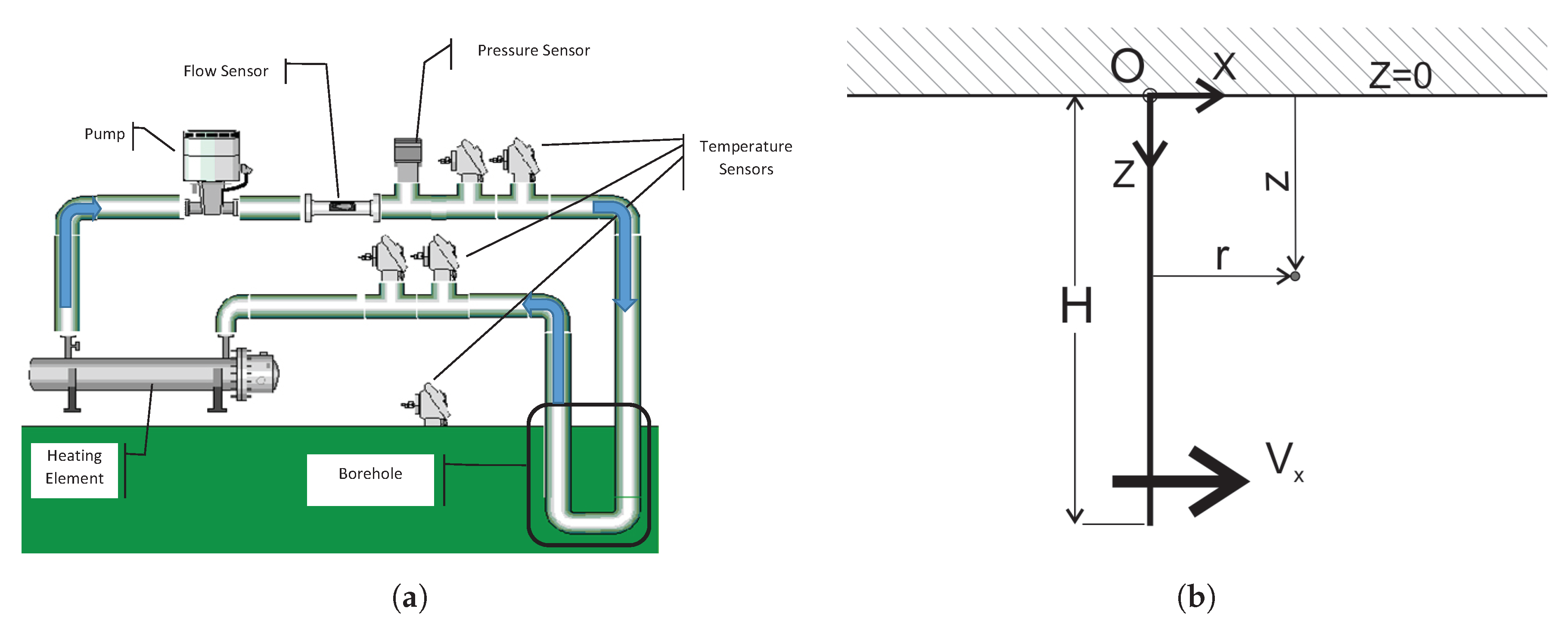
• A constant heat flow rate per unit length of the borehole ${\dot{q}}_L=\frac{\dot{Q}}{H}$ is applied to a linear source of either infinite or finite length. If we choose a finite linear source, it stretches along the z-axis down to the same depth as the physical length of the BHE to be represented, H;
• The linear source moves in relation to the semi-infinite permeable soil with a velocity which is equal to the uniform velocity of Darcy $u_x$.

Regarding item 4, though it is clear that BHEs are not linear, in the context of TRT analysis, one may be not particularly interested in the details of how heat transfer takes place inside the BHE region, i.e., within distances shorter than the borehole radius, $r_b$. Methods based on linear sources cannot properly represent heat transfer at distances smaller than $r<r_b$ and at times too short for the heat flow to be established within the surrounding soil (represented by the short timescale $t_b$), but may work well beyond this lower time limit. In this case, it is sufficiently accurate to represent the additional specific heat resistance within the borehole (that depends on the geometry of the BHE, the grout characteristics, etc.) by means of a single parameter termed borehole thermal resistance, $R_b$. Any model representing the thermal response of the BHE seeks a prediction of the temperature at any time $t(>t_b)$ after the start of heat injection measured at the observation location within the soil with cylindric coordinates ($r>r_b$, z, $\varphi$), which in general takes the form:

$$T(r,z,\varphi ,t)=\mathsf{\Delta }T(r,z,\varphi ,t)+T_0+{\dot{q}}_L{R}_b,$$

(4)

and depending on the model at use, $\mathsf{\Delta }T$ will include the effect of quantities such as soil conductivity, borehole length, and ground water flow. To compare the outcome with the measured temperature increase, we additionally have to consider some way of averaging Expression (4) along the borehole and/or angle coordinates, since ${\overline{T}}_{exp}$ depends only on time. One approach is to use the value calculated at some typical depth such as the midth of the BHE length [18,19,20]. A second, possibly more precise, but computationally more cumbersome option is to calculate the BHE–averaged $〈\mathsf{\Delta }T(t)〉$ quantities and to compare experimental data with a model in the form:

$${\overline{T}}_{exp}=〈\mathsf{\Delta }T(r_b,t)〉+T_0+{\dot{q}}_L{R}_b.$$

(5)

In the literature, the above expression is usually represented in terms of the so-called g-functions that represent the temperature increase in a nondimensional form $〈\mathsf{\Delta }T(r_b,t)〉=\frac{{\dot{q}}_L}{2\pi \lambda }g(t)$. G-functions do not depend on the actual heat injection rate TRT, and so they can be conveniently used for BHE design.

2.3. Infinite (ILS) Line-Source Models

Within the ILS and FLS schemes, we neglect heat transport through advection (thus considering $u_x=0$) and the heat transport problem becomes axisymmetric. In the case of the ILS model, the configuration additionally possesses translational symmetry along the z-coordinate (which consequently does not appear in the solution).

To solve the inner problem of heat transfer inside the BHE in the ILS case—see [17,46]—the average temperature of the fluid, ${\overline{T}}_{exp}$, is expressed using the temperature at the lateral surface of the borehole and the experimental temperature increase is given by:

$$\begin{array}{cc}\hfill {\overline{T}}_{exp}& =\mathsf{\Delta }{T}_{ILS}(r_b,t)+T_0+{\dot{q}}_L{R}_b\hfill \\ \hfill & =\frac{{\dot{q}}_L}{4\pi \lambda }{E}_i(-\frac{r_b^2}{4\alpha t})+T_0+{\dot{q}}_L{R}_b\approx \frac{{\dot{q}}_L}{4\pi \lambda }(ln\frac{4\alpha t}{r_b^2}-\gamma )+T_0+{\dot{q}}_L{R}_b,\hfill \end{array}$$

(6)

where the function $E_i(u)$ denotes the exponential integral [15], $\gamma$ is the Euler–Mascherotti’s constant and the symbol $O(x)$ denotes terms proportional to the argument x and higher powers of x. It is to be noted that the term ${\mathrm{Fo}}_b=\frac{\alpha t}{r_b^2}$ represents the Fourier number with respect to the borehole radius $r_b$, as $t_b=\frac{r_b^2}{\alpha }$ is the timescale (early timescale) related to $r_b$. It is commonly considered that the ILS representation is valid for times that are larger than 5 times $t_b$ (i.e., ${\mathrm{Fo}}_b>5$), usually in the order of some hours to 1 day [18,20], whereas typical thermal test durations range from 40 to over 200 h [7,47].

2.4. Finite Linear-Source (FLS) Scheme

In the FLS model, the configuration loses its z–translational symmetry and the temperature field depends on the depth. Consequently, we must include some average procedure in order to compare the model result with the experimental ${\overline{T}}_{exp}$ measure. To this aim, it is best to use the mean integral temperature [18,19,46]:

$$〈\mathsf{\Delta }{T}_{FLS}(r_b,t)〉=\frac{1}{H}{\int }_0^H\mathsf{\Delta }{T}_{FLS}(r_b,z,t)dz,$$

(7)

where there is now a second timescale associated with the borehole depth, H, $t_H=\frac{H^2}{\alpha }$, which is much larger than $t_b$. In general, the duration of a TRT lies within intermediate times such that $(t_b<t\ll t_H)$ to distinguish them from very long times ($t>t_H$), in which the temperature at any distance would reach a steady-state value [18,19]. Such asymptotic behavior is characteristic of FLS models and does not exist in the ILS theory, but even with a duration of about 30 days, the longest of our TRT tests at UPV is far from reaching the long timescale.

An exact analytic solution for the temperature averaged over the borehole depth was approximated for the intermediate time range in Reference [19], which is a simple and easy-to-compute asymptotic form for the mean borehole temperature:

$$\begin{array}{cc}\hfill {\overline{T}}_{exp}& =〈\mathsf{\Delta }{T}_{FLS}(r_b,t)〉+T_0+{\dot{q}}_L{R}_b\hfill \\ \hfill & =\frac{{\dot{q}}_L}{4\pi \lambda }\left(-\gamma -2log\frac{r_b}{H}+log\frac{4t}{t_H}+\frac{3r_b}{H}-\frac{3}{\sqrt{\pi }}\sqrt{\frac{4t}{t_H}}-\frac{3}{\sqrt{\pi }}\frac{r_b^2}{H^2}\sqrt{\frac{4t}{t_H}}\right)\hfill \\ \hfill & +T_0+{\dot{q}}_L{R}_b\hfill \end{array}$$

(8)

It results from the above expression that the TRT response in the FLS case can be represented in terms of just two nondimensional quantities: The nondimensional borehole radius ($\beta =\frac{r_b}{H}$) and a Fourier number related to the long timescale given by:

$${\mathrm{Fo}}_H=\frac{t}{t_H}=\frac{\alpha t}{H^2},$$

(9)

and in terms of these numbers, we can rewrite the expressions for the ILS and FLS models more simply as:

$$\mathsf{\Delta }{T}_{ILS}({\mathrm{Fo}}_H)=\frac{{\dot{q}}_L}{4\pi \lambda }\left(log(4{\mathrm{Fo}}_H)-2log(\beta )-\gamma \right),$$

(10)

which allows the FLS temperature response Function (8) to be written—taking into account that $\beta \ll 1$ and $\mathrm{Fo}\ll 1$—as a correction term to the latter in the form:

$$\begin{array}{cc}\hfill 〈\mathsf{\Delta }{T}_{FLS}({\mathrm{Fo}}_H)〉=& \mathsf{\Delta }{T}_{ILS}({\mathrm{Fo}}_H)+\hfill \\ \hfill & \frac{{\dot{q}}_L}{4\pi \lambda }\left(3\beta +{\beta }^2\left(\frac{1}{4{\mathrm{Fo}}_H}-\frac{3}{2\sqrt{\pi }\sqrt{{\mathrm{Fo}}_H}}\right)-\frac{6\sqrt{{\mathrm{Fo}}_H}}{\sqrt{\pi }}\right).\hfill \end{array}$$

(11)

2.5. Infinite (MILS) Moving Line-Source Method

The importance of groundwater for heat transport phenomena and particularly for BHEs has been a focus of attention for a long time. In the pioneering work of Claesson and Eskilson [20], an additional term was introduced to account for the effect of groundwater flow, depending on groundwater convective velocity and other parameters. Later, Chiasson, [39], Hähnlein [48] and, more recently, Molina-Giraldo, [49] and Zhang [36] performed numerical or analytical studies to evaluate its effects on heat transfer or on the extension and geometry of temperature disturbance around the BHE. In a recent review, Wagner [41] discussed these approaches and did an extensive survey on the effects of different factors, including groundwater velocity on the temperature disturbance.

Groundwater flow velocities are highly variable depending on the hydrogeological conditions, due mainly to hydraulic conductivity, which can range over several orders of magnitude [39]. For instance, the hydraulic conductivity of sandy sediments can vary from ${10}^{-5}$ m/s to ${10}^{-3}$ m/s. Assuming a constant and typical hydraulic gradient of ${10}^{-3}$, the Darcy velocity ranges from ${10}^{-8}$ m/s to ${10}^{-6}$ m/s for fine and coarse sands, respectively. For the analytic treatment of the heat transport in the framework of Equation (3), it is convenient to introduce a further nondimensional quantity, the Péclet number, given as:

$$\mathrm{Pe}=v_t\frac{H}{\alpha },$$

(12)

According to Chiasson [39], “The Péclet number has been used to quantify the relative importance of mechanical (or advective) dispersion versus molecular diffusion in mass transport in ground water.” In previous studies conducted by Bear [50], it was found that when choosing grain size as the characteristic length, diffusion was the process controlling mass transport at Péclet numbers less than about 0.4, whereas at Péclet numbers in the range of 0.4 to 5, a transition occurred. Above a Péclet number of about 5, mechanical dispersion (or advective dispersion) dominated. In Reference [39] (Table 2–2, page 32), the calculated Péclet numbers were listed using the typical borehole spacing of 4.5 m as a reference length. Data indicated that heat advection by ground water flow is significant in coarse-grained soils (sands and gravels) and in rocks exhibiting secondary porosities (fracturing and solution channels), although as stated by Chiasson, “When the characteristic length is defined as the borehole spacing, Peclet numbers exceeding 1 exist only for sands, gravels, and karst limestones. It is possible however, that even when the Péclet number is of order one or higher, the effects of the ground-water flow on the temperature response may not be seen within the normal time scale of an in-situ thermal conductivity test.”

In this context, a more general analytic approach, such as that elaborated by Molina-Giraldo [49] (extending the previous work of the authors of [51,52]), is especially useful to obtain some general conclusions. Following these authors, the general solution to Equation (3) for a moving infinite line source is given by:

$$\mathsf{\Delta }{T}_{\mathrm{MILS}}(\rho ,{\mathrm{Fo}}_H,\mathrm{Pe},\varphi )=\frac{{\dot{q}}_L}{4\pi \lambda }{exp}^{\frac{\mathrm{Pe}}{2}\rho cos\left[\varphi \right]}{\int }_0^{\frac{1}{4}{\mathrm{Fo}}_H{\mathrm{Pe}}^2}\frac{1}{\psi }{exp}^{\left(-\frac{{\mathrm{Pe}}^2{\rho }^2}{16\psi }-\psi \right)}d\psi ,$$

(13)

where the angle $\varphi$ represents the angular position of the observation point with respect to the direction of the groundwater flow at the observation distance represented by $\rho =\frac{r}{H}$. To compare with the experimentally determined temperature, we can use the average of the temperature field over the borehole perimeter at the borehole radius $r_b$ and the following expression is obtained:

$$\begin{array}{cc}\hfill 〈\mathsf{\Delta }{T}_{\mathrm{MILS}}(\beta ,{\mathrm{Fo}}_H,\mathrm{Pe})〉& =\frac{{\dot{q}}_L}{4\pi \lambda }\frac{1}{\pi }\hfill \\ \hfill & {\int }_0^{\pi }{exp}^{\frac{\mathrm{Pe}}{2}\beta cos\left[\varphi \right]}d\varphi \times {\int }_0^{\frac{1}{4}{\mathrm{Fo}}_H{\mathrm{Pe}}^2}\frac{1}{\psi }{exp}^{\left(-\frac{{\mathrm{Pe}}^2{\beta }^2}{16\psi }-\psi \right)}d\psi .\hfill \end{array}$$

(14)

This expression can be readily computed numerically as a product of two functions for which we can write:

$$〈\mathsf{\Delta }{T}_{\mathrm{MILS}}(\beta ,{\mathrm{Fo}}_H,\mathrm{Pe})〉=\frac{{\dot{q}}_L}{4\pi \lambda }\mathsf{\Theta }(\mathrm{Pe},\beta )g_{MILS}({\mathrm{Fo}}_H,\mathrm{Pe},\beta ),$$

(15)

with:

$$\begin{array}{c}\hfill \mathsf{\Theta }(\mathrm{Pe},\beta )=\frac{1}{\pi }{\int }_0^{\pi }{exp}^{\frac{\mathrm{Pe}}{2}\beta cos\left[\varphi \right]}d\varphi \approx 1\end{array}$$

(16)

$$\begin{array}{c}\hfill g_{MILS}({\mathrm{Fo}}_H,\mathrm{Pe},\beta )={\int }_0^{\frac{1}{4}{\mathrm{Fo}}_H{\mathrm{Pe}}^2}\frac{1}{\psi }{exp}^{\left(-\frac{{\mathrm{Pe}}^2{\beta }^2}{16\psi }-\psi \right)}d\psi .\end{array}$$

(17)

Condition (16) holds whenever $\mathrm{Pe}/2\beta \ll 1$, which is usually the case for BHEs of a typical depth of tens of meters (implying $\beta \ll 1$) and in usual soils with not too extreme hydraulic conductivities.

2.6. Finite (MFLS) Moving Line-Source Method

Stepping further, the work of Molina-Giraldo (2012) [49] studies the moving finite line source (MFLS) departing from the general solution for Green’s function of an instantaneous point source within a moving medium. Following the procedure outlined in his contribution, the solution of the heat transport given is given by:

$$\begin{array}{cc}\hfill \mathsf{\Delta }{T}_{\mathrm{MFLS}}(\rho ,{\mathrm{Fo}}_H,\mathrm{Pe},\varphi ,z)=& \frac{{\dot{q}}_L}{4\pi \lambda }{exp}^{\frac{\mathrm{Pe}}{2}\rho cos\left[\varphi \right]}\times \hfill \\ \hfill & \left({\int }_0^H{F}_{\mathrm{MFLS}}(\rho ,\zeta ,Z,{\mathrm{Fo}}_H,\mathrm{Pe})d\zeta \right.\hfill \\ \hfill & -\left.{\int }_{-H}^0{F}_{\mathrm{MFLS}}(\rho ,\zeta ,Z,{\mathrm{Fo}}_H,\mathrm{Pe})d\zeta \right)\hfill \end{array}$$

(18)

where:

$$\begin{array}{cc}\hfill F_{\mathrm{MFLS}}(\rho ,\zeta ,Z,{\mathrm{Fo}}_H,\mathrm{Pe})& =\frac{1}{2\sqrt{{\rho }^2+{(Z-\zeta )}^2}}\hfill \\ \hfill & \left(e^{\frac{1}{2}(-\mathrm{Pe})\sqrt{{\rho }^2+{(Z-\zeta )}^2}}\mathrm{erfc}\left(\frac{\sqrt{{\rho }^2+{(Z-\zeta )}^2}-{\mathrm{Fo}}_H\mathrm{Pe}}{2\sqrt{{\mathrm{Fo}}_H}}\right)\right.\hfill \\ \hfill & +\hfill \\ \hfill & \left.e^{\frac{1}{2}\mathrm{Pe}\sqrt{{\rho }^2+{(Z-\zeta )}^2}}\mathrm{erfc}\left(\frac{{\mathrm{Fo}}_H\mathrm{Pe}+\sqrt{{\rho }^2+{(Z-\zeta )}^2}}{2\sqrt{{\mathrm{Fo}}_H}}\right)\right),\hfill \end{array}$$

(19)

and where $erfc(.)$ represents the error function, $\rho$ the nondimensional radial coordinate, and Z the the nondimensional z–coordinate of the observation point ($Z=z/H$) and $\zeta$ the nondimensional z-coordinate of the line-source elements. After angular averaging and numerical integration along the line-source coordinate, the temperature change can be expressed in the form:

$$\begin{array}{cc}\hfill 〈\mathsf{\Delta }{T}_{\mathrm{MFLS}}(\rho ,{\mathrm{Fo}}_H,\mathrm{Pe},z)〉=& \frac{{\dot{q}}_L}{4\pi \lambda }\mathsf{\Theta }(\mathrm{Pe},\rho )\times \hfill \\ \hfill & \left(g_{\mathrm{MFLS}}^{+}(\rho ,Z,{\mathrm{Fo}}_H,\mathrm{Pe})-g_{\mathrm{MFLS}}^{-}(\rho ,Z,{\mathrm{Fo}}_H,\mathrm{Pe}).\right)\hfill \end{array}$$

(20)

Finally, to compare with experimental results, we observe that the contribution of the mirror line source $g_{MFLS}^{-}$ is very small except for very shallow observation points ($Z\approx 0$). On the other hand, although it would be necessary to compute the Z-average of $g_{MFLS}^{+}$ to be consistent with the averaging criteria outlined before, this would result in a rather high computational cost, given that the function must be evaluated many times within fitting algorithms. Instead, following the original criteria by Eskilson [17], we might use the function value at mid-depth of the BHE ($Z=\frac{1}{2}$) as a reasonable approximation. We thus arrive at expression:

$$〈\mathsf{\Delta }{T}_{\mathrm{MFLS}}({\mathrm{Fo}}_H,\mathrm{Pe})〉\approx \frac{{\dot{q}}_L}{4\pi \lambda }\mathsf{\Theta }(\mathrm{Pe},\beta )\times g_{\mathrm{MFLS}}^{+}(\beta ,\frac{H}{2},{\mathrm{Fo}}_H,\mathrm{Pe}),$$

(21)

where:

$$g_{\mathrm{MFLS}}^{+}(\beta ,\frac{H}{2},{\mathrm{Fo}}_H,\mathrm{Pe})={\int }_0^H{F}_{\mathrm{MFLS}}(\beta ,\zeta ,\frac{H}{2},{\mathrm{Fo}}_H,\mathrm{Pe})d\zeta .$$

(22)

As pointed out in Reference [49] (Figure 6, pp. 2511) only from ${\mathrm{Fo}}_H>5\times {10}^{-2}$ are the differences between the temperatures predicted by the infinite moving line-source (MILS) and MFLS approaches expected to become noticeable. Nevertheless, in our analysis, we use both models to approximate TRT experimental data.

Our following objective is to compare the result of using Expressions (10), (11), (15), and (21) against data of TRTs of a longer than standard duration of up to 32 days.

3. Measurements Description

This section shows a description of our thermal installation and hydrogeological information of the site, followed by a detailed description of the heat injection tests carried out, and ending with a presentation of the analysis methodology used.

3.1. Description of Borehole Exchanger Facility and Hydrogeology of the Site

The test facility—completed in May 2010—is located inside the city of Valencia’s UPV campus. All the information on the description of the installation is provided in Section 2.1 of Reference [45].

As a summary, we can extract from Reference [45] the table with the characteristics of the main measuring equipment installed in the hydraulic circuit (see

Table 1. List of the sensors and their main characteristics.

Sensor Name	Units	Description	Specification
$T_{i{n}_1}$	${}^{\circ }$C	Temperature at borehole inlet	IFM TA3130 [53] PT100 Class A Range: 0–140 ${}^{\circ }$C Output: 4–20 mA Res < 0.02 ${}^{\circ }$C
$T_{i{n}_2}$
$T_{ou{t}_1}$	${}^{\circ }$C	Temperature at borehole outlet
$T_{ou{t}_2}$
$T_{und}$	°C	Ground temperature
$T_{amb}$	${}^{\circ }$C	Ambient temperature
Pressure	Pa	System pressure	OSAKA PP10 [54] Range: 0–1000 kPa Output: 4–20 mA Linearity: 0.3% Stability: 0.2%
Flow	m3 h−1	Water Flow	IFM SM8000 [55] Range: 0.01–6.00 m3 h−1 Output: 4–20 mA Res < 0.005 m3 h−1

).

Samples of ground components were collected while drilling, providing a fair insight into the ground layer structure. The geological setting of the test site corresponds to continental alluvial deposits, such as sands, silts, conglomerates, peat deposits, all of them Quaternary in age and related to the activity of the major river (Turia) in addition to small ravines that have governed the geomorphology of the Valencian region during the Quaternary [56]. The water table of the area is around 2 m, so it is understood that the soil is saturated from that depth. The lithostratigraphic column of the test site consists of the following units described from bottom to top:

• From 40 to 36 m deep: A layer of gravels with a coarse sand matrix, generally assumed to correspond to paleochannels or secondary distributary channels associated to the activity of the ravines.
• From 36 to 26 m deep: The next layer is dominated by sandy deposits passing upward to silty and clay deposits, which are related to the flooding plains associated to the alluvial environments.
• From 26 to 12 m deep: A layer of rounded gravels with a 5 cm edge.
• From 12 to 4 m deep: After the second episode of gravels, the sedimentation was related to peat deposits. Those peats were deposited in marsh areas (ancient or recent), previously studied by the authors of [57]. Some of them are still present along the coast of Valencia and Castellón, forming high valuable natural environments, such as the Albufera.
• From 4 m deep to surface: Finally, the top of the column is formed by 4 m of fine sediments (clays and silts) associated, again, with flooding plains.

In summary, the geological characteristics of the study area correspond to an alluvial environment dominated by the sedimentation of siliciclastic materials with different granulometries associated to the activities of the rivers and ravines occurring in this area. All those materials conform an open aquifer that was described in the hydrogeological map of Spain as the Aquifer system of Plana de Valencia [58]. Those materials are considered permeable to semipermeable, allowing a continuous groundwater flow seawards according to the information that can be extracted from the hydrogeological map and the local record of piezometric levels in several wells and control points. In our study, we compiled all the geological and hydrogeological information of the test site to tentatively decipher a series of hydrodynamic parameters to be incorporated to the modeling of the groundwater flow effect in TRTs. According to published information relating lithologies with permeability values (as an approach of the hydraulic conductivity) [50], well-sorted unconsolidated materials such as those that are present in our test site possess values oscillating between ${10}^6$ to ${10}^3$ milidarcy. Those materials can be considered pervious to semipervious materials in concordance with Bear’s approach. According to these estimations, hydraulic conductivity values are expected to be in the range of $0.001$ to 1 cm/s [50].

3.2. Previous Estimation of Thermal Soil Parameters

In Reference [59], a thermal characterization of core samples obtained from a test site close to our TRT site is described. The measurements were performed in a laboratory following the ASTM D 5334-08 thermal needle method or the dual-probe method [60], indistinctly. In both, the thermal properties of the sample were determined indirectly by measuring the rise or fall of temperature at the point of interest in response to a line-source heat input. Taking into account that the conformation of the soil materials is very close in both sites, the thermal conductivity in our site could be approximated from the sample conductivities of the materials obtained from the different layers (${\lambda }_i$, the different core samples are shown in Reference [59], Table 5, pp. 7), extrapolated to the layer structure of our test site, as shown in Figure 1a of Reference [45], by means of expression:

$$\overline{\lambda }=\frac{1}{H}{\displaystyle \sum _i^N}{\lambda }_i{h}_i,$$

(23)

${\lambda }_i$ and $h_i$ being the conductivity and depth of each layer, respectively, N the total number of layers (N = 6), and H the total borehole length ($H=39.5$ m). Using the center values for each of the layers according to Reference [59] (Table 5, pp. 7), the conductivity estimate obtained for our case is: $\overline{\lambda }=2.37$ W/(m.K).

In addition, with reference to the geohydrology and Darcy velocities expected, the study of Chiasson [39] established a correspondence between lithologies and Péclet numbers, according to which we can infer that the Péclet number in our system could vary between 4500 (in gravel dominating layers) and 8 (for sand and clays dominating layers) if a characteristic length corresponding to borehole depth, H, is used. Due to the layered soil structure, it is nevertheless difficult to estimate an a-priori value for an average or effective Péclet number.

3.3. Heat Injection Fluctuation Control Scheme and Description of Tests

In Reference [44], we extensively examined the importance of the heat injection control scheme to ensure quality of data. Its role is to keep the heat injection rate into the ground as stable as possible within the duration of the entire TRT test. The importance of the PID controller in our installation can be seen in Figures 5 and 6 of Reference [45], where the cleanliness of the results is observed, without disturbances by the outside temperature.

A key finding in Reference [61] was that all experiments performed using the PID control showed not only better stability, but also a notably improved match between data and the different theoretical models used to adjust the experiments and estimate parameters. It was found that FLS models have a slightly better least square error (LSQ) and, thus, allow an improved estimation of parameters. On the other hand, the values of ground conductivity and borehole resistance found were in a similar range when using ILS or FLS.

In the present work, we extend this analysis considering moving line-source models and tests of a longer duration than considered in the previous work. Furthermore, we only consider tests performed with PID control, disregarding those in which heat resistance was operated at constant power.

Table 2. Brief description of included experiments.

Experiment Name	Start Date (yyyy-mm-dd)	Duration (Days)	Control	Heat Injection Rate
				Mean (W)	Std. Dev.
test_1_2	2016-03-07	11	PID	1982	26
test_2_15	2017-03-07	9	PID	1497	24
test_2_25	2017-04-10	32	PID	2428	22

summarizes the main characteristics of the TRT experiments included in our present analysis. The duration of the tests performed is variable, ranging from 9 to 31 days, and, nevertheless, longer than the typical 72 h used by commercial TRTs mobile devices, in compliance with the recommendations included in the current standards, such as the IEA-ECES Annex 21 Final Report, see [62].

To prepare data for comparison with models, the dataset is divided into two parts, before and after the start of heat injection. Data from the period before the injection start can be useful to gather information about the initial temperatures around the borehole. The second dataset only takes into account the period after the heat injection starts and is the basis for the parameter identification algorithms we describe in the next sections.

A basic process variable is the mean temperature in the BHE, ${\overline{T}}_{exp}$, calculated as the average between $T_{in}$ and $T_{out}$, considering the sensors closest to the inlet and outlet of the BHE. The injected heat rate is calculated for each sampling period using Equation (24), averaged over the complete time series to determine the value ${\dot{q}}_l$ to be used within the models.

$${\dot{q}}_L=\frac{1}{n}\frac{{\displaystyle \sum _{i=1}^n}(T_{{in}_i}-T_{{out}_i}){\dot{g}}_i{c}_{f_i}}{H},$$

(24)

where $T_{{in/out}_i}$ is the temperature in °C at the inlet/outlet of the borehole, ${\dot{g}}_i$ is the fluid flow in m³s⁻¹, and $c_{f_i}$ is the volumetric heat capacity of the fluid. All quantities refer to each time bin, i, in which the data sample is divided.

3.4. Parameter Estimation Procedure

To each dataset divided into n temperature readings, we applied the following procedure:

• The value for the soil diffusivity is set at $\alpha =6\times {10}^{-7}\frac{{\mathrm{m}}^2}{\mathrm{s}}$. The rest of geometrical parameters, H and $r_b$ and the resulting value of $\beta =\frac{r_b}{H}$ are set according to the geometry of the TRT site;
• The mean heat injection rate is calculated following Expression (24);
• A derived data vector is calculated given by: $\left\{F{o}_{H_i},T_{{exp}_i}\right\}$ (for $i=1\dots n$), $F{o}_{H_i}$ being the Fourier number corresponding to time $t_i$ (according to Expression (9)) and $T_{{exp}_i}$ being the average inlet and outlet temperatures at time $t_i$. The calculated data vector is truncated, leaving only those readings for which $t_i>5t_b$.
• A least square (LSQ) optimization algorithm is applied to the data. Given a theoretical model (“mod”), the algorithm finds those model parameter values $\left\{\lambda ,\mathrm{Pe},T_1\right\}$—where $T_1$ represents an absolute temperature penalty parameter given by $T_1=T_0+{\dot{q}}_L{R}_b$—that minimize the error given by Equation (25) between the predicted temperatures for each of the three available model options (Expressions (10), ( 11), and (21)) and the experimental dataset. The LSQ error is given by:

  $${\overline{ϵ}}^2=\frac{1}{N}{\displaystyle \sum _{i=1}^N}{(T_{{exp}_i}-T_{{mod}_i})}^2.$$

  (25)

  In the case of the ILS and FLS methods, no estimate for the Péclet number is obtained.
• To test whether a stable parameter estimation is obtained, the described procedure is repeated with a varying number of days in the data file, starting from day 3 up to the last day of the test. The resulting information is stored in a data structure of the form:

  $$par\left[i\right].mod\left[j\right].test\left[k\right]\left[d\right],$$

  which is a matrix containing the estimation for parameters ($\lambda ,R_b$, and $Pe$) as well as statistical estimators, such as $LSQ$, p-values, and confidence intervals (pointed at with the parameter index i), gathered using reference model j (either ILS, FLS, MILS, or MFLS) and based on the experimental results of test k (restricted here to the tests listed in Table 2). The day index d signals that only experimental data gathered up to day d are taken into account for that estimation.

The full algorithm was implemented using version 11.2 of the Wolfram Mathematica software package [63], and in particular function NonLinearModelFit, to construct the estimated parameter sets.

4. Results and Discussion

This section presents the main results obtained. First of all, the comparison between the analytical models and the experimental results obtained is detailed. From this analysis, the estimation of the main parameters is obtained, such as the ground thermal conductivity, the characterization of the groundwater flow, and the thermal resistance of the borehole heat exchanger, completing it with a deep analysis of the error between analytical models and experimental results.

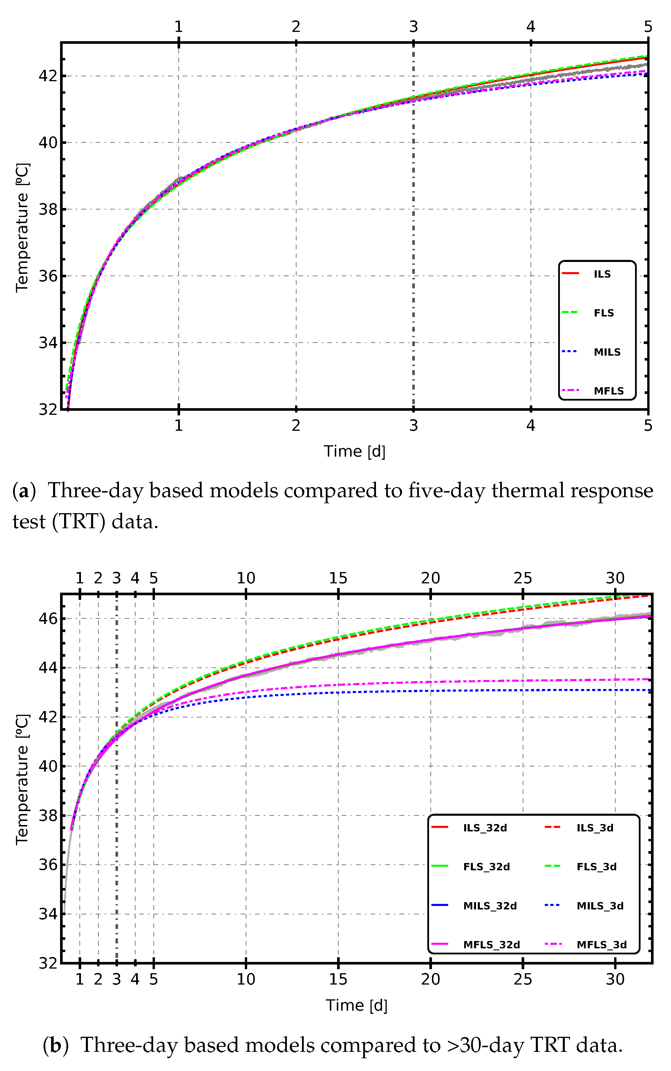
4.1. Experiment vs. Model

Figure 2 compares modeling and experimental results for the longest test (test_2_25). The theoretically predicted curves were obtained by means of the LSQ optimization procedure, as described in the previous section. Figure 2a depicts the result of the analysis for the first 72 test hours, corresponding to a standard three-day TRT test duration (although, for clarity, data are extended to a five-day window). Regardless of the model utilized, there is a good visual match between the data and the models if optimum values for the soil conductivity, borehole resistance, and Péclet number parameters are used. However, if the curves are extrapolated outside of the data window for which the parameters were calculated to the full 32-day period (as shown in Figure 2b), the predicted temperatures and actually measured ones are substantially different. In models taking into account groundwater flow, predicted temperatures would fall below the measured ones, while the ILS and FLS models would clearly overpredict future temperatures around the BHE.

However, if the soil and BHE parameters are estimated from the full 32-day dataset, again we see that the predicted temperatures match the response of the borehole accurately (which can be also seen in Figure 2b) . In fact, the predictions of the four models considered are basically indistinguishable, and what varies depending on which model is used are the estimated parameters and its statistics. We can conclude that the models can always be adjusted to follow temperature evolution accurately within the time window for which they are trimmed, but parameters found for different time windows may vary substantially and produce considerably different predictions for future temperatures.

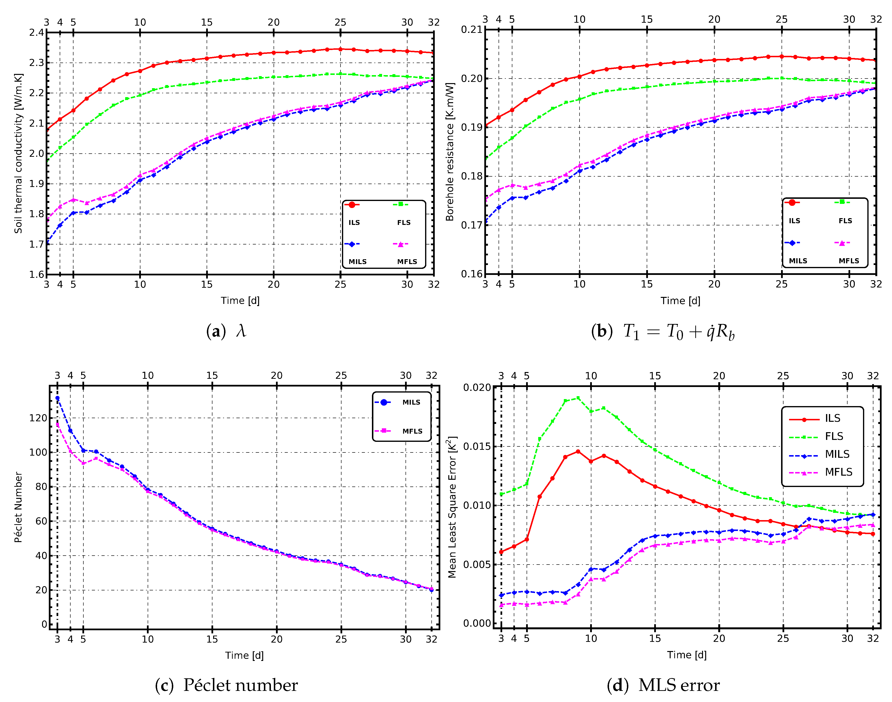
4.2. Soil Thermal Conductivity and Groundwater Flow Parameter

In order to better represent these tendencies, the four figures in Equation (3) show the value of the extracted soil and BHE parameters from experiments of a varying duration. The shortest test considered corresponds to the standard 72 h duration of a TRT. As a function of the number of days, extracted parameters $\lambda$ and $T_1=T_0+\dot{q}{R}_b$ show markedly parallel trends. For models ILS and FLS, they increase up to day 12 to stabilize at approximately the same value up to day 32. For models taking into account groundwater flow (MILS and MFLS), the soil parameter estimates increase steadily at a slower rate, reaching similar values to those of models ILS and FLS at the end of the 32-day test period. By contrast, the Péclet number obtained from the LSQ optimization of the MILS and MFLS models (Figure 3c) shows no clear final estimate. The quality of the parameter estimations, as given by the LSQ values, shown in Figure 3d, indicates that the MILS and MFLS models adjust better to experimental data, especially at short and intermediate times, but at the price of introducing high values of the Péclet number and a substantially different configuration of the $\lambda -R_b$ parameter estimates. As the experiment proceeds, LSQ and the rest of the parameters tend to have similar values compared to those of the ILS and FLS models. It is thus to be suspected that this improved short-term agreement between data and MILS/MFLS models is a product of spurious over-fitting more than an indication of strong groundwater flow effects.

Comparing the estimation for the ILS and FLS models, the results show a small but systematic decrease of the soil conductivity values (a final value $2.22\frac{W}{m.K}$ compared to $2.33\frac{W}{m.K}$), regardless of whether we consider finite-line corrections or not. This difference does not appear if we compare estimates of the MILS and MFLS models, which are basically coincident for all the considered parameters. Hence, axial effects play no role during our tests within the framework of moving line-source theories, which is in complete agreement with theoretical considerations, as highlighted in Section 2.6.

In Figure 4, we have represented $R_b$ as a function of $\lambda$ parametrically, where each point corresponds to the estimated parameter values of one of the models and for a given test duration. There is a clear grouping of all data within a straight line, which is to be expected from the structure of the models, since borehole resistance and soil resistance appear as additive contributions to the same experimentally measured temperatures. With increasing duration, the points tend to accumulate in a parameter region where the true soil and $R_b$ parameters are most likely expected to be. This small region is similar for all models, but is reached much faster by models without groundwater flow (ILS and FLS) than by the MILS and MFLS models.

It is important here to examine three aspects in relation with this prediction: Its stability against experimental errors, its reproducibility in different tests, and how fast the predicted parameter region is reached depending on the used model, or how the analysis is done. This later aspect is crucial in TRT practice, as it gives an indication of what the required duration of a TRT should be.

4.3. Error Analysis and Comparison Between Different Experiments

To examine the sensitivity of the predicted soil parameter values against experimental errors—either random or systematic—a Monte Carlo type approach was followed by constructing a large number of perturbed datasets from the original full 32-day experimental data. Each of these sets was obtained from the original measurements by adding an independent random error to the true experimental values of the inlet and outlet temperature and volume flow sensor readings. The errors were chosen with a probability corresponding to a normal distribution which took into account the uncertainties determined by sensor calibration. After obtaining each perturbed dataset, the parameter extraction procedure was applied and a new set of $(\lambda ,R_b,\mathrm{Pe})$ estimations was obtained. The density of pairs obtained in a given region in the ($\lambda ,R_b,\mathrm{Pe}$) parameter space, thus, represents the probability that the true parameter values are located there, given the known experimental uncertainties.

In Figure 5, such a probability density region is shown as the result of a simulation in which 400 different perturbed datasets were obtained and its parameters estimated, taking into account the temperature calibrated accuracy of $\pm 0.1$ K and a flow sensor accuracy of $\pm 2\%$. The contour lines represent the percentage of simulated parameters pairs that lie within each part of the elliptic shaped region. The outermost contour line represents a 95% probability region that the true values are found within. The same calculation with the MILS and MFLS models produces an ellipsoidal volume (results not shown). Errors in the $\lambda$ and $R_b$ estimates are inversely correlated in the sense that higher soil conductivity estimates would be combined with lower $R_b$ estimates, giving a valuable statistical indication where, within a given experimental situation, we expect the soil parameters to be.

Furthermore, depending on which model is used, the parameter confidence region is approached rather slowly. In Figure 6, the residua for the 32-day data, representing the difference between the measured ${\overline{T}}_{exp}$ and the model-predicted temperatures, depict similar tendencies—a noisy fluctuation superimposed upon a similar low frequency pattern—indicating that during the first five days of the TRT, there is a positive systematic deviation from the experimental data that vanishes in later days. This deviation is not attributable to groundwater flow or axial effects, since these are already contained in the models. As it is affecting the short-term behavior of the models, this effect is possibly connected to the idealized description of the heat source used, not taking into account its real geometry. A cylinder source approximation or other approaches—like CaRM or a cylinder-source approach—considering the actual BHE geometry would possibly not exhibit such short timescale deviations. In the TRT context, it indicates that the problems in parameter estimation could be improved if we dismiss data taken at those times within the parameter estimation procedure.

To evaluate the effect of this systematic residua structure in the estimation of soil parameters, we repeated the parameter estimation outlined before, but disregarding all experimental data obtained during the first test day. We observed (see Figure 7 and Figure 8) that this changed some of facts we could outline before. Although the final result in terms of estimated values of the parameters was similar to those obtained in the previous analysis (at least in the case of $\lambda$ and $R_b$), it is clear that the disclosure of data from the first day caused a much faster approach to the final parameter values in all four models and for all the parameters under consideration. A striking difference is that from day 25, the MILS and MFLS models arrived to a more stable prediction for the Pe-number around $\mathrm{Pe}=0.3$. Despite its small magnitude, this value has a high p-value and is quite insensitive to the rest of experimental uncertainties, signaling a modest, but detectable influence of groundwater flow effects within the timescale of the test, which are nevertheless below the range of possible values that could be deduced from pure geological considerations. Confirming previous observations, we can also see that the ILS, MILS, and MFLS models systematically agree on the values of the soil conductivity parameter and BHE resistance.

Finally, to analyze reproducibility, we repeated the analysis leading to Figure 4, but using data from tests 2_15 and 1_2, covering a range of specific heat injection rates between 30 and 65 W/m. The result is shown in Figure 9, confirming the same characteristic linear trend between the $\lambda$ and $R_b$ parameters, but slightly shifted within the different experimental sets.

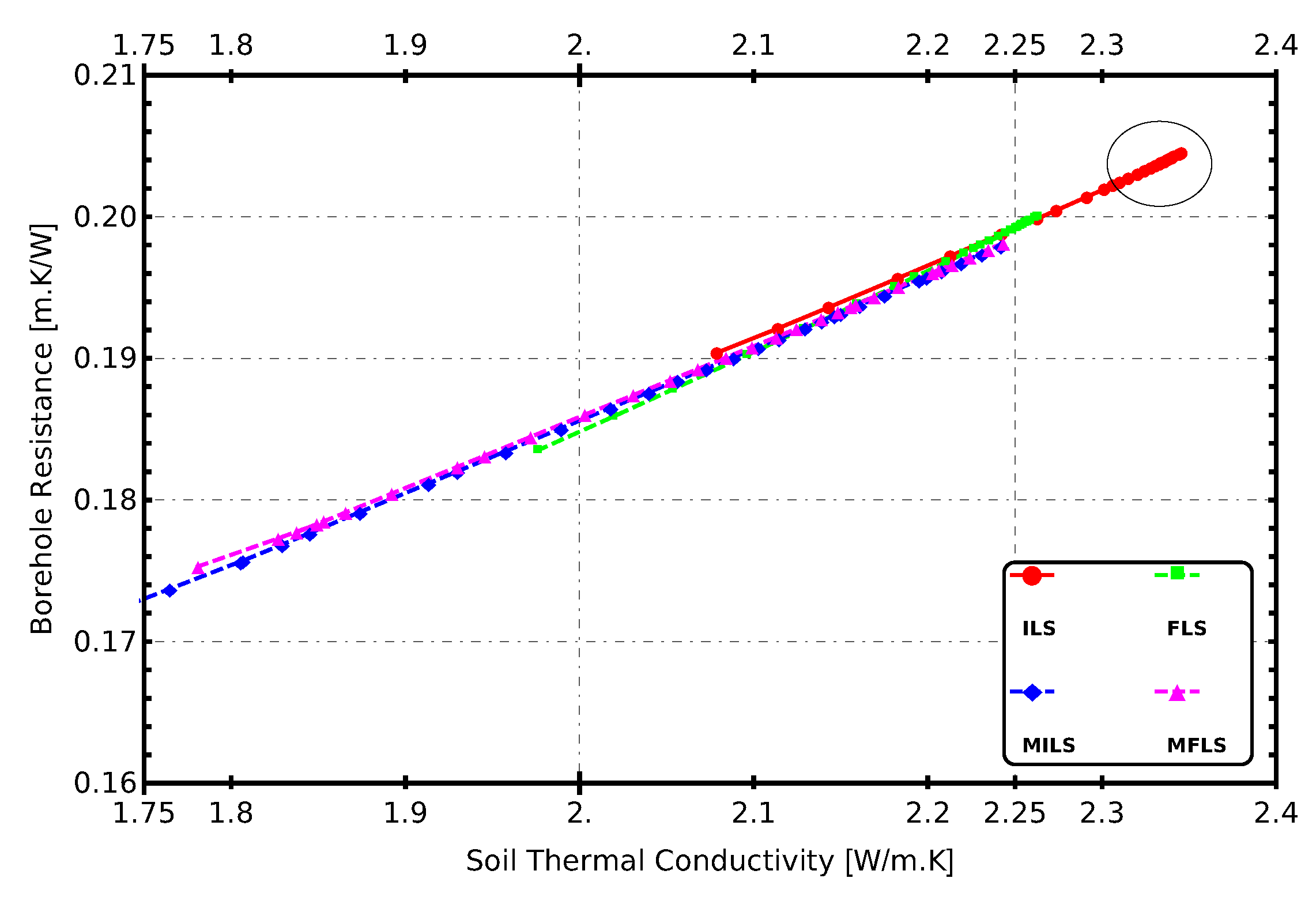
4.4. Borehole Resistance Estimation

It is important to note that the borehole resistance estimation from which Figure 3b was obtained is based on the assumption of a certain value of the undisturbed ground temperature ($T_0=20.12{}^{\circ }$C), derived from the experimental results of direct underground temperature sensing, as discussed in Reference [43]. A different assumption for $T_0$ leads to different values of $R_b$ and it is thus crucial to use an estimation of the undisturbed soil temperature that matches, as close as possible, the real situation.

In this context, there is no reason to assume that $T_0$ is strictly constant, as there are several factors that could affect its value, such as seasonal temperature fluctuations (especially if the system is very shallow), geothermal gradients, and even previous heat injections that may have altered the soil temperature field in the neighborhood of our BHE. Disturbances to the soil temperature due to the presence of other heat sources or caused by the effects of the local hydrogeology are also possible.

Regarding the seasonal oscillations of ground temperature, the following expression [64] allows to calculate the temperature at depth z, corresponding to time t within the ground subject to a periodic seasonal oscillation of temperatures of amplitude $A_s$ with yearly average temperature $\overline{T}$:

$$T(z,t)=\overline{T}-A_s{e}^{-\sqrt{\frac{\pi }{365}}\sqrt{\frac{1}{\alpha }}z}cos\left(\frac{2}{365}\pi \left(t-t_0-\frac{1}{2}\sqrt{\frac{365}{\pi }}\sqrt{\frac{1}{\alpha }}z\right)\right),$$

(26)

where t and $t_0$ are usually expressed in days. The average temperature oscillation around the mean temperature in a volume of ground of depth H (corresponding to the BHE length) is then given by:

$$\mathsf{\Delta }T(t,H)=\frac{1}{H}{\int }_0^{H}T(z,t)dz=\frac{A_s\sqrt{\frac{365\alpha }{2\pi }}sin\left(\frac{2}{365}\pi (t-\mathrm{t}0)+\frac{\pi }{4}\right)}{H}+O(e^{-H}).$$

(27)

The amplitude of the BHE-averaged seasonal temperature oscillation is hence given by $\frac{A_s}{H}\sqrt{\frac{365\alpha }{2\pi }}$, which for data corresponding to the Valencia climate (with a span of about $A_s=7{}^{\circ }$C and $H=39.5$ m) corresponds to an amplitude of about $\pm 0.3$ K around the average undisturbed ground temperature $\overline{T}$.

The influence of such a disturbance on the estimation of the borehole resistance can be observed in Figure 9, where the gray zone around the test_2_15 curve shows the effect of a change in the assumption of $T_0$ by $\pm 0.1$ K in the ($\lambda -R_b$) parameter estimation trajectories.

In conclusion, a change (of up to $0.6$ K) in the undisturbed ground temperature between measurement made in different seasons can produce a vertical shift in the $R_b$ parameter estimation, as shown in Figure 9 and, regarding TRT practice in general, it clearly highlights the need to take into account uncertainties in undisturbed ground temperature if precision in $R_b$ estimation is pursued.

5. Conclusions and Further Outlook

In this work, we presented a number of TRT experiments performed at the Universitat Politècnica de València (Polytechnic University of Valencia) BHE test site, from which we could highlight the following main observations:

• We reported the result of three experiments performed with a reduction active PID control of the external thermal fluctuation. As reported in a previous communication, this is essential to obtain useful conclusions from the analyzed data;
• Four theoretical models—all based on the line-source approach—were chosen to analyze the resulting information because of their relative simplicity and due to being amongst those most usually used in TRT practice;
• The most significant test for the analysis of the performance of the different models was the 32-day long stable heat pulse TRT. From the analysis of this test, it was possible to conclude the following:
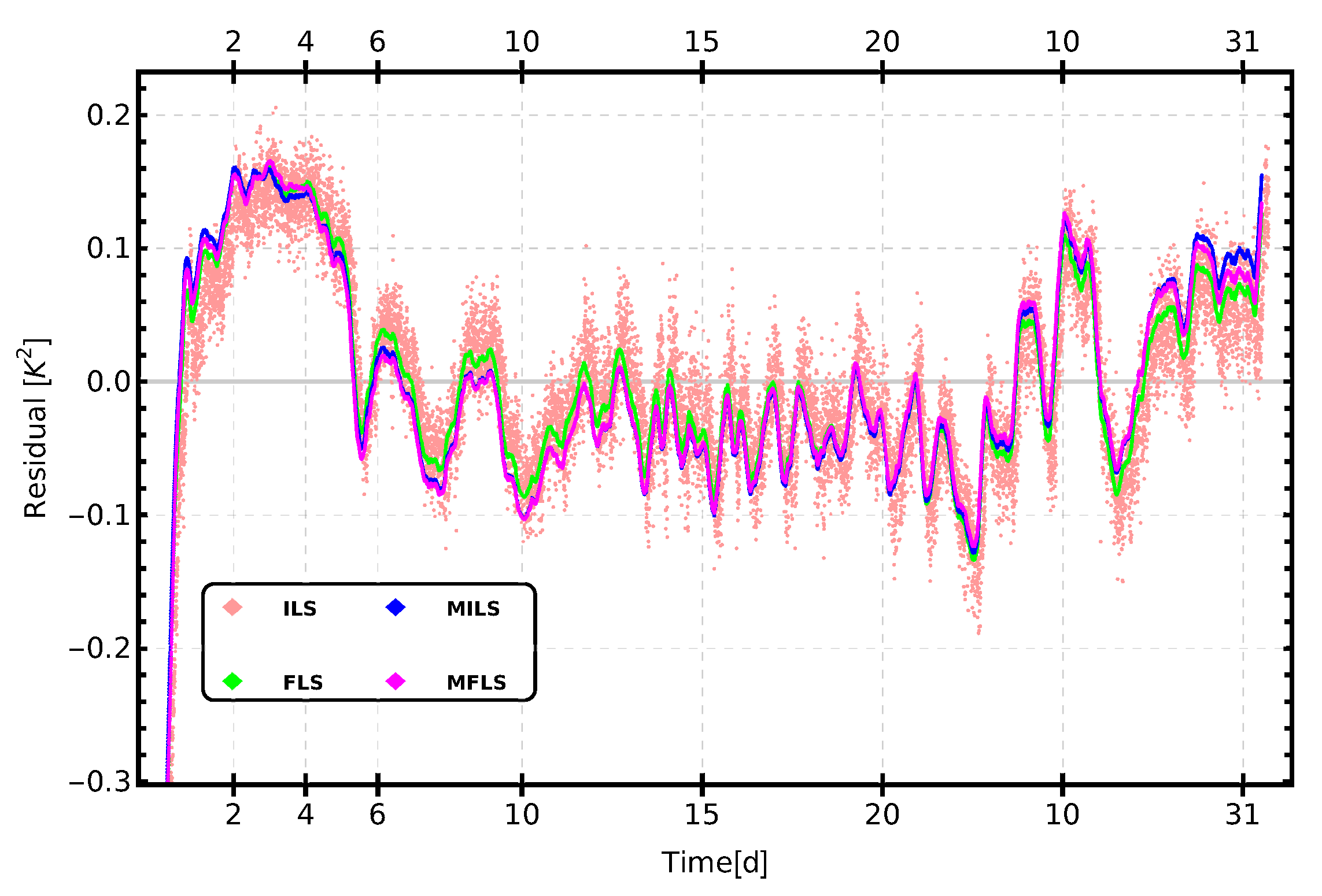
  • All four models can accurately represent experimental temperature evolution, in the sense that on a visual inspection, theoretical and calculated curves are coincident. However, there are many caveats regarding the significance parameters extracted and its reproducibility and stability;
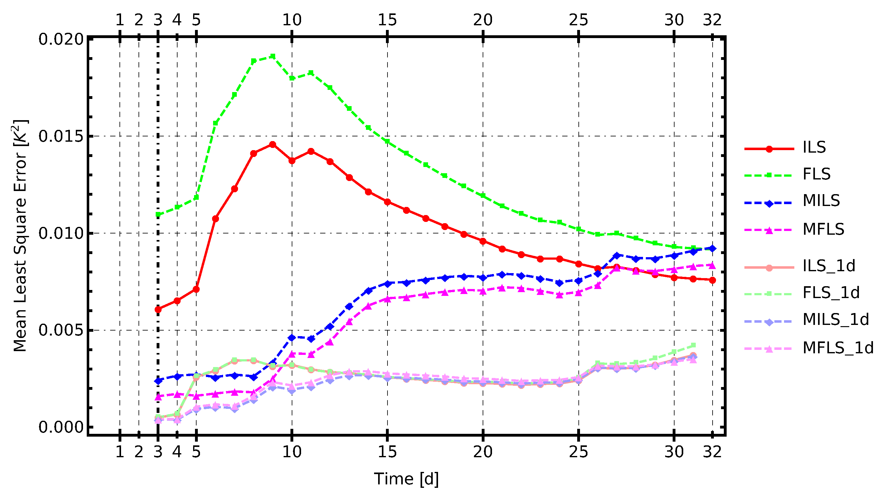
  • If no adequate data selection is done, parameters extracted from the tests from the first days are substantially different than parameters that are extracted taking into account a longer period. The ILS and FLS models only stabilize their predictions after 10–12 days, whereas for the MILS and MFLS models, it takes substantially longer to find a stable parameter estimate;
  • If data from the first test days are disregarded for the analysis, the convergence to the definitive parameter estimates is much faster. This is probably due to the fact that heat transfer during the first 2–3 days is not adequately represented by a line-source model;
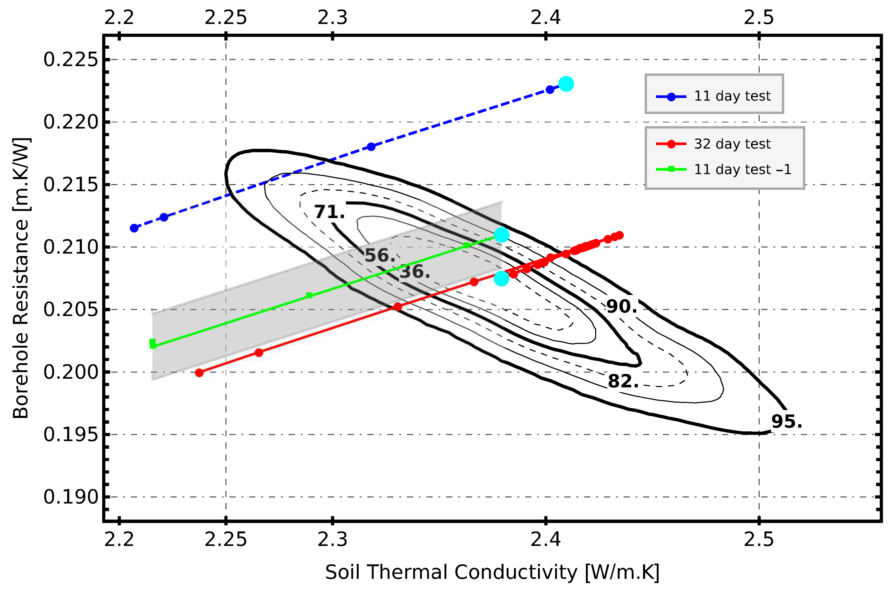
  • After 32 days, the ILS, MILS, and MFLS converged to the same values for the $\lambda$ and $R_b$ soil and BHE resistance parameters. The final value of $2.37\pm 0.07$ W/(m.K) is in a good agreement with estimates from soil tests [59]. For the borehole resistance, $R_b=0.206\pm 0.006$ (m.K)/W was obtained;
  • Soil conductivity estimates by the FLS theories are similar, but systematically lower than the former ($2.32\pm 0.06$ W/(m.K)), signaling that the axial effects are small, but detectable with these tests;
  • The MILS and MFLS theories produced a consistent and stable estimate for the Péclet number of $Pe=0.2939\pm 0.0001$. The value obtained is quite robust towards experimental errors and model uncertainties and, thus, could be considered significant.
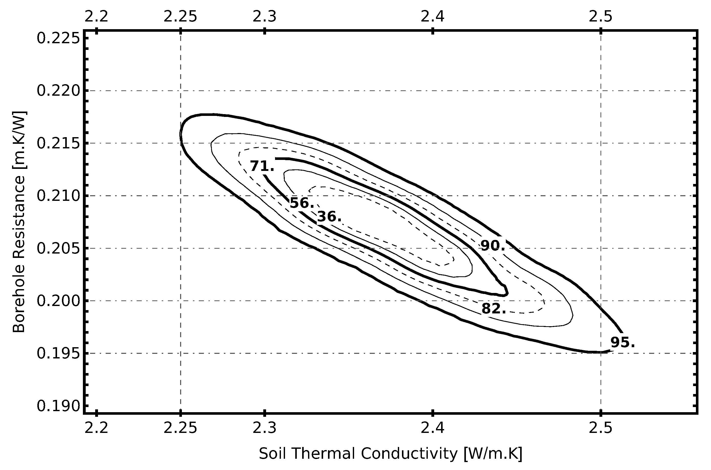
• We constructed an experiment-independent parameter confidence region for the estimates of ($\lambda ,R_b,\mathrm{Pe}$) that characterized the sensitivity of the results of parameter estimation to systematic or random experimental errors. The different experiments showed reproducible results in the sense that the accumulation points of the parameter estimates of all models fell within the same confidence region. It is, however, essential to get high-precision results, to take into account seasonal and other sources of perturbation of the undisturbed ground temperature $T_0$ used for the calculations;
• As a final outcome of our analysis, we can confirm the good qualities of the ILS approach to be used as reference model for parameter estimation in our soil conditions: It is very simple to handle, displays a comparable LSQ in longer tests, and more importantly, it shows a faster convergence towards the parameter confidence region when test duration is shorter, since in geothermal industry, for economic and operational reasons, TRT tests are carried out in the shortest possible time, and this could lead to the estimation of incorrect thermal parameters regarding the long-term behaviour of the system.

With our test site, many other types of analysis can be performed: Using models or correlations to describe the short-term performance of the BHE could, in principle, improve the features detected with the used schemes and stabilize parameter estimation. A detailed hydrogeological and hydrogeodynamical study of the location is planned in order to corroborate the most accurate values for the parameters related to the ground flow, such as measurements of the permeability of the different layers, measurement of the flow velocity and direction, and determination of the degree of saturation of the different layers or strata. A further possible investigation is to test methods (such as based on heat pulses of different amplitudes) to obtain a faster approach to reliable parameter estimates.

References

1. Omer, A.M. Ground-source heat pumps systems and applications. Renew. Sustain. Energy Rev. 2008, 12, 344–371. [Google Scholar] [CrossRef]
2. Sanner, B.; Karytsasb, C.; Mendrinosb, D.; Rybach, L. Current status of ground source heat pumps and underground thermal energy storage in Europe. Geothermics 2003, 32, 579–588. [Google Scholar] [CrossRef]
3. Urchueguía, J.; Zacarés, M.; Corberĺn, J.; Montero, Á.; Martos, J.; Witte, H. Comparison between the energy performance of a ground coupled water to water heat pump system and an air to water heat pump system for heating and cooling in typical conditions of the European Mediterranean coast. Energy Convers. Manag. 2008, 49, 2917–2923. [Google Scholar] [CrossRef]
4. Lim, H.; Kim, C.; Cho, Y.; Kim, M. Energy saving potentials from the application of heat pipes on geothermal heat pump system. Appl. Therm. Eng. 2017, 126, 1191–1198. [Google Scholar] [CrossRef]
5. Lund, J.W. Direct heat utilization of geothermal resources. Renew. Energy 1997, 10, 403–408. [Google Scholar] [CrossRef] [Green Version]
6. A Guide to Energy-Efficient Heating and Cooling; Technical report; U.S. Environmental Protection Agency (EPA): Washington, DC, USA, 2009.
7. Sanner, B.; Hellström, G.; Spitler, J.D.; Gehlin, S. More than 15 years of mobile Thermal Response Test—A summary of experiences and prospects. In Proceedings of the European Geothermal Congress, Pisa, Italy, 3–7 June 2013. [Google Scholar]
8. Thermal Response Test (TRT) State-of-the Art 2011: IEA ECES ANNEX 21; Technical report; Luleå University of Technology, Architecture and Water: Luleå, Sweden, 2011.
9. Witte, H.J. Error analysis of thermal response tests. Appl. Energy 2013, 109, 302–311. [Google Scholar] [CrossRef]
10. Borinaga-Treviño, R.; Pascual-Muñoz, P.; Castro-Fresno, D.; Blanco-Fernandez, E. Borehole thermal response and thermal resistance of four different grouting materials measured with a TRT. Appl. Therm. Eng. 2013, 53, 13–20. [Google Scholar] [CrossRef]
11. Witte, H.J.L.; Van Gelder, G.J.; Spitier, J.D. In situ measurement of ground thermal conductivity: A Dutch perspective. Ashrae Trans. 2002, 108, 263. [Google Scholar]
12. Hellström, G. Ground Heat Storage: Thermal Analyses of Duct Storage Systems. Ph.D. Thesis, Lund University, Longde, Sweden, 1991. [Google Scholar]
13. Conti, P.; Testi, D.; Grassi, W. Revised heat transfer modeling of double-U vertical ground-coupled heat exchangers. Appl. Therm. Eng. 2016, 106, 1257–1267. [Google Scholar] [CrossRef]
14. Ingersoll, L.; Zobel, O.; Ingersoll, A. Heat Conduction: With Engineering, Geological and Other Applications; Madison University of Wisconsin Press: Madison, WI, USA, 1954. [Google Scholar]
15. Carslaw, H.S.; Jaeger, J.C. Conduction of Heat in Solids; OXFORD UNIV PR: Oxford, UK, 1986. [Google Scholar]
16. Mogenson, P. Fluid to Duct Wall Heat Transfer in Duct System Heat Storages. In Proceedings of the International Conference on Subsurface Heat Storage in Theory and Practice, Stockholm, Sweden, 6–8 June 1983. [Google Scholar]
17. Eskilson, P. Thermal Analysis of Heat Extraction Boreholes. Ph.D. Thesis, Lund University, Longde, Sweden, 1987. [Google Scholar]
18. Lamarche, L.; Beauchamp, B. A new contribution to the finite line-source model for geothermal boreholes. Energy Build. 2007, 39, 188–198. [Google Scholar] [CrossRef]
19. Bandos, T.V.; Montero, Á.; Fernández, E.; Santander, J.L.G.; Isidro, J.M.; Pérez, J.; de Córdoba, P.J.F.; Urchueguía, J.F. Finite line-source model for borehole heat exchangers: effect of vertical temperature variations. Geothermics 2009, 38, 263–270. [Google Scholar] [CrossRef]
20. Eskilson, P.; Claesson, J. Simulation model for thermally interacting heat extraction boreholes. Numer. Heat Transf. 1988, 13, 149–165. [Google Scholar] [CrossRef]
21. Gehlin, S.; Nordell, B. Determining undisturbed ground temperature for thermal response test. In Proceedings of the Winter Meeting of the American Society of Heating, Refrigerating and Air-Conditioning Engineers, Orlando, FL, USA, 5–9 February 2005. [Google Scholar]
22. Sanner, B.; Hellström, G.; Spitler, J.; Gehlin, S. Thermal Response Test—Current Status and World-Wide Application. In Proceedings of the World Geothermal Congress, Antalya, Turkey, 24–29 April 2005. [Google Scholar]
23. Austin, W. Development of an In-Situ System for Measuring Ground Thermal Properties. Master’s Thesis, Oklahoma State University, Stillwater, OK, USA, 1998. [Google Scholar]
24. Shonder, J.; Beck, J. Field test of a new method for determining soil formation thermal conductivity and borehole resistance. Ashrae Trans. 2000, 106, 929. [Google Scholar]
25. Beier, R.A. Transient heat transfer in a U-tube borehole heat exchanger. Appl. Therm. Eng. 2014, 62, 256–266. [Google Scholar] [CrossRef]
26. Carli, M.D.; Tonon, M.; Zarrella, A.; Zecchin, R. A computational capacity resistance model (CaRM) for vertical ground-coupled heat exchangers. Renew. Energy 2010, 35, 1537–1550. [Google Scholar] [CrossRef]
27. Rivera, J.A.; Blum, P.; Bayer, P. Analytical simulation of groundwater flow and land surface effects on thermal plumes of borehole heat exchangers. Appl. Energy 2015, 146, 421–433. [Google Scholar] [CrossRef]
28. Beier, R.A.; Smith, M.D. Borehole thermal resistance from line-source model of in-situ tests. Ashrae Trans. 2002, 108, 212. [Google Scholar]
29. Javed, S.; Fahlén, P.; Holmberg, H. Modelling for optimization of brine temperature in ground source heat pump systems. In Proceedings of the 8th International Conference on Sustainable Energy Technologies (SET 2009), Istanbul, Turkey, 8–9 June 2009. [Google Scholar]
30. Zeng, H.Y.; Diao, N.R.; Fang, Z.H. A finite line-source model for boreholes in geothermal heat exchangers. Heat Transf. Asian Res. 2002, 31, 558–567. [Google Scholar] [CrossRef]
31. Witte, H.; van Gelder, A. Geothermal Response Tests using controlled multipower level heating and cooling pulses (MPL–HCP). In Proceedings of the 10th International Conference on Thermal Energy Storage, Ecostock 2006, Pomona, NJ, USA, 31 May–2 June 2006. [Google Scholar]
32. Noorollahi, Y.; Saeidi, R.; Mohammadi, M.; Amiri, A.; Hosseinzadeh, M. The effects of ground heat exchanger parameters changes on geothermal heat pump performance—A review. Appl. Therm. Eng. 2018, 129, 1645–1658. [Google Scholar] [CrossRef]
33. Jahangir, M.H.; Sarrafha, H.; Kasaeian, A. Numerical modeling of energy transfer in underground borehole heat exchanger within unsaturated soil. Appl. Therm. Eng. 2018, 132, 697–707. [Google Scholar] [CrossRef]
34. Zarrella, A.; Pasquier, P. Effect of axial heat transfer and atmospheric conditions on the energy performance of GSHP systems: A simulation-based analysis. Appl. Therm. Eng. 2015, 78, 591–604. [Google Scholar] [CrossRef]
35. Bandos, T.; Montero, A.; Fernández de Córdoba, P.; Urchueguía, J. Improving parameter estimates obtained from thermal response tests: Effect of ambient air temperature variations. Geothermics 2011, 40, 136–143. [Google Scholar] [CrossRef] [Green Version]
36. Zhang, Y.; Li, L.; Erler, D.V.; Santos, I.; Lockington, D. Effects of alongshore morphology on groundwater flow and solute transport in a nearshore aquifer. Water Resour. Res. 2016, 52, 990–1008. [Google Scholar] [CrossRef] [Green Version]
37. Wood, C.J.; Liu, H.; Riffat, S.B. Comparative performance of ‘U-tube’ and ‘coaxial’ loop designs for use with a ground source heat pump. Appl. Therm. Eng. 2012, 37, 190–195. [Google Scholar] [CrossRef]
38. Abdelaziz, S.L.; Ozudogru, T.Y. Selection of the design temperature change for energy piles. Appl. Therm. Eng. 2016, 107, 1036–1045. [Google Scholar] [CrossRef]
39. Chiasson, A.D. Advances in Modeling of Ground-Source Heat Pump Systems. Master’s Thesis, Faculty of the Graduate College of the Oklahoma State University, Stillwater, OK, USA, 1999. [Google Scholar]
40. Molina-Giraldo, N.; Blum, P.; Zhu, K.; Bayer, P.; Fang, Z. A moving finite line source model to simulate borehole heat exchangers with groundwater advection. Int. J. Therm. Sci. 2011, 50, 2506–2513. [Google Scholar] [CrossRef]
41. Wagner, I.M. Oberflächennahe Geothermiesondenanlagen : von der Praxisstudie zur modellbasierten Analyse ihrer Temperaturfahnenausbreitung. Ph.D. Thesis, Institut und Versuchsanstalt für Geotechnik der Technischen Universität Darmstadt, Darmstadt, Germany, 2016. [Google Scholar]
42. Luo, J.; Tuo, J.; Huang, W.; Zhu, Y.; Jiao, Y.; Xiang, W.; Rohn, J. Influence of groundwater levels on effective thermal conductivity of the ground and heat transfer rate of borehole heat exchangers. Appl. Therm. Eng. 2018, 128, 508–516. [Google Scholar] [CrossRef]
43. Montero, A.; Urchueguía, J.F.; Martos, J.; Badenes, B.; Picard, M.A. Ground temperature profile while thermal response testing. In Proceedings of the European Geothermal Congress 2013, Pisa, Italy, 3–7 June 2013; pp. 1–6. [Google Scholar]
44. Badenes, B.; Mateo Pla, M.A.; Magraner, T.; Lemus, L.; Urchueguía, J.F. Experimental facility to perform Thermal Response Tests and study the thermal behaviour of the ground. In Proceedings of the European Geothermal Congress 2016, Strasbourg, Feance, 19–23 September 2016. [Google Scholar]
45. Badenes, B.; Mateo Pla, Á.M.; Lemus-Zúñiga, G.L.; Sáiz Mauleón, B.; Urchueguía, J.F. On the Influence of Operational and Control Parameters in Thermal Response Testing of Borehole Heat Exchangers. Energies 2017, 10. [Google Scholar] [CrossRef]
46. Zeng, H.; Diao, N.; Fang, Z. Heat transfer analysis of boreholes in vertical ground heat exchangers. Int. J. Heat Mass Transf. 2003, 46, 4467–4481. [Google Scholar] [CrossRef]
47. Signorelli, S.; Bassetti, S.; Pahud, D.; Kolh, T. Numerical evaluation of Thermal Response Tests. Geothermics 2007, 36, 141–166. [Google Scholar] [CrossRef]
48. Hähnlein, S.; Molina-Giraldo, N.; Blum, P.; Bayer, P.; Grathwohl, P. Ausbreitung von Kältefahnen im Grundwasser bei Erdwärmesonden [Cold plumes in groundwater for ground source heat pump systems]. Grundwasser 2010, 15, 123–133. [Google Scholar] [CrossRef]
49. Molina-Giraldo, N.; Blum, P.; Bayer, P. Importance of thermal dispersion in temperature plumes. In Proceedings of the 8th International Conference on Calibration and Reliability in Groundwater Modeling, Brisbane, Australia, 2–10 August 2012; Volume 355, pp. 195–200. [Google Scholar]
50. Bear, J. Dynamics of Fluids in Porous Media; Dover Civil and Mechanical Engineering Series: Dover, UK, 1972. [Google Scholar]
51. Sutton, M.G.; Nutter, D.W.; Couvillion, R.J. A Ground Resistance for Vertical Bore Heat Exchangers With Groundwater Flow. J. Energy Resour. Technol. 2003, 125, 183–189. [Google Scholar] [CrossRef]
52. Diao, N.; Li, Q.; Fang, Z. Heat transfer in ground heat exchangers withgroundwater advection. Therm. Sci. 2004, 43, 203–1211. [Google Scholar]
53. TA3130-Temperature Transmitter-IFM Electronic. Available online: https://www.ifm.com/gb/en/product/TA3130 (accessed on 29 November 2018).
54. OSAKA PP10. Available online: http://osakasolutions.com/wp-content/uploads/2012/11/Manual_ PP30-PP10-PP08.pdf (accessed on 29 November 2018).
55. IFM SM8000-Flow Transmitter-IFM Electronic. Available online: https://www.ifm.com/gb/en/product/SM8000 (accessed on 29 July 2018).
56. Geological Map of Spain. Scale 1:50.000, MAGNA. Page n°722 (Valencia); IGME: Madrid, Spain, 1972.
57. López-Buendía, A.; Whateley, M.; Bastida, J.; Urquiola, M. Origins of mineral matter in peat marsh and peat bog deposits, Spain. Int. J. Coal Geol. 2007, 71, 246–262. [Google Scholar] [CrossRef]
58. Hydrogeological Map of Spain. Scale 1:200.000. Page n°56 (Valencia); IGME: Madrid, Spain, 2015.
59. Badenes, B.; de Santiago, C.; Nope, F.; Magraner, T.; Urchueguía, J.F.; de Groot, M.; de Santayana, F.P.; Arcos, J.L.; Martín, F. Thermal characterization of a geothermal precast pile in Valencia (Spain). In Proceedings of the European Geothermal Congress, Strasbourg, Feance, 19–23 September 2016. [Google Scholar]
60. Bristow, K.L.; Kluitenberg, G.J.; Horton, R. Measurement of Soil Thermal Properties with a Dual-Probe Heat-Pulse Technique. Soil Sci. Soc. Am. J. 1994, 58, 1288–1294. [Google Scholar] [CrossRef]
61. Badenes, B.; Belliardi, M.; Bernardi, A.; Carli, M.D.; Tuccio, M.D.; Emmi, G.; Galgaro, A.; Graci, S.; Pockele, L.; Vivarelli, A.; Pera, S.; Urchueguía, J.F.; Zarrella, A. Definition of Standardized Energy Profiles for Heating and Cooling of Buildings. In Proceedings of the 12th REHVA World Congress 2016, Aalborg, Denmark, 22–25 May 2016. [Google Scholar]
62. Tinti, F.; Bruno, R.; Focaccia, S. Thermal response test for shallow geothermal applications: a probabilistic analysis approach. Geotherm. Energy 2015, 3, 6. [Google Scholar] [CrossRef]
63. Wolfram Research, I. Mathematica 11.2. Available online: https://www.wolfram.com/mathematica (accessed on 29 November 2018).
64. Hillel, D. Fundamentals of Soil Physics; Academic Press: Cambridge, MA, USA, 1982; pp. 287–317. [Google Scholar]
Figure 1. Experimental facility hydraulic system, basic diagram (a) (where the arrows indicate water flow direction) and (b) coordinate system used as reference for the theoretical calculations.
Energies 11 03347 g001
Figure 2. Comparison of experimental mean BHE temperatures (gray area) vs. the prediction of four different calculation models. In a standard TRT, the model parameters are estimated using only the first three days of test (72 h), which give the comparison graph shown in (a). In (b), the same three-day based models are compared to models fitted from the whole data of a 32-day experiment and the raw data.
Energies 11 03347 g002
Figure 3. Comparison of the evolution of the parameter estimates when the number of days of the experiment is increased for each of the four different models. The data are taken from test_2_25. In (a) soil conductivity ( λ ), in (b) the borehole resistance estimation ( T 1 = T 0 + q ˙ R b ), and in (c) the Péclet number estimation (only for the two models that use this value). The mean least square error between theoretical models and measured data for the four different models is shown in (d). The legends are the same in the four curves.
Energies 11 03347 g003
Figure 4. Trajectories of the successive ( λ , R b ) estimates in the corresponding parameter plane. The circle represents the parameter region around which the parameter estimates accumulate for a longer test duration.
Energies 11 03347 g004
Figure 5. Probability density regions for λ ,   R b after 400 simulations of perturbed datasets for a temperature calibrated accuracy of ± 0.1 K and a flow sensor accuracy of ± 2 % .
Energies 11 03347 g005
Figure 6. Residue plot, meaning the difference between measured and modeled temperatures for the 32-day test and model parameters estimated from the full 32-day dataset. Two of the plots (infinite moving line source (MILS) and moving finite line source (MFLS)) have been smoothed to highlight the average tendency, whilst the two others (infinite line source (ILS) and finite line source (FLS)) are directly represented.
Energies 11 03347 g006
Figure 7. Mean least square error between theoretical models and measured data for the four different models as a function of the data time window used, but considering only data gathered after day 1 for the analysis (light colors). To compare, the previous least square error (LSQ) data from Figure 3d are included.
Energies 11 03347 g007
Figure 8. (a) Soil conductivity estimation for the four different models as a function of the data time window used with data only from day 1. (b) Péclet number estimation for the four different models as a function of the data time window used.
Energies 11 03347 g008
Figure 9. Combination of probability density regions (Figure 5) and ( λ R b ) estimation trajectory for the 32-day test (red line), the original 11-day test (blue line), and the 11-day test with –1-day data (green line). The cyan circles show the estimated final values for each test. The gray filled region around the 11-day with –1-day test trajectory shows the result of the estimation if the undisturbed ground temperature would have been taken ± 0.1 K around the estimated value of 20.12 °C.
Energies 11 03347 g009