Abstract
The aerodynamic interaction between wind turbines grouped in wind farms results in wake-induced power loss and fatigue loads of wind turbines. To mitigate these, wind farm control should be able to account for those interactions, typically using model-based approaches. Such model-based control approaches benefit from computationally fast, linear models and therefore, in this work, we introduce the Dynamic Flow Predictor. It is a fast, control-oriented, dynamic, linear model of wind farm flow and operation that provides predictions of wind speed and turbine power. The model estimates wind turbine aerodynamic interaction using a linearized engineering wake model in combination with a delay process. The Dynamic Flow Predictor was tested on a two-turbine array to illustrate its main characteristics and on a large-scale wind farm, comparable to modern offshore wind farms, to illustrate its scalability and accuracy in a more realistic scale. The simulations were performed in SimWindFarm with wind turbines represented using the NREL 5 MW model. The results showed the suitability, accuracy, and computational speed of the modeling approach. In the study on the large-scale wind farm, rotor effective wind speed was estimated with a root-mean-square error ranging between 0.8% and 4.1%. In the same study, the computation time per iteration of the model was, on average, s. It is therefore concluded that the presented modeling approach is well suited for use in wind farm control.
1. Introduction
The wind energy market has been growing rapidly at a rate of 16% throughout the past decade, reaching 539,123 MW of global installed capacity in 2017 [1]. Modern wind turbines are complex machines with sophisticated control systems. Single turbine control systems are well developed and most of the modern machines are, at least to some extent, optimized in the areas of aerodynamics [2], aeroelasticity [3], and control [4]. When grouped in wind farms, the individual optimal operation does not necessarily coincide with the overall optimum, mainly due to the aerodynamic interaction between the wind turbines. Control actions on one wind turbine may impact the performance of another wind turbine in its vicinity; therefore, considering such interaction effects is beneficial in wind farm control. The operation of the whole wind farm is optimized in wind farm control using a coordinated control algorithm that specifies the operation point of each turbine. Common objectives of wind farm control are (i) to maximize the total power of the wind farm [5,6] or (ii) to follow a specified reference for the total power of the wind farm that is termed power control [7,8]. The control objectives can be augmented to include multiobjective optimization that simultaneously also aims to reduce the fatigue loads of wind turbines [9,10,11]. In approaches of wind farm control with the objective of the maximization of the total power, it is crucial to consider the aerodynamic interaction of wind turbines in the model employed for control [12,13].
The turbulent nature of wind farm flow [14] drives the benefit of predicting wind speed dynamics at wind turbines in certain areas of wind farm control. The investigated prediction approaches are individual turbine-based prediction [15,16,17] and wind farm-scale, dynamic flow models [18,19]. The former approaches use measurements at the respective wind turbine or in the turbine’s proximity to predict the evolution of wind speed at that turbine. The prediction is performed using statistical models [15,20] and/or machine learning [21]. An overview of relevant prediction methods can be found in Reference [22]. Such an individual turbine-based prediction does not, however, model the aerodynamic interaction of wind turbines.
With regard to the power control of wind farms, model-free [7,8] and model-based approaches [9,10,11] have been investigated in literature. Model-based approaches typically employ dynamic models, since they result in a superior performance compared to static models [23]. The use of model-based approaches for the power control of wind farms can provide several advantages over model-free approaches. First, the use of models of the aerodynamic interaction of wind turbines allows to optimally distribute the extraction of kinetic power from wind flow in space and time in a wind farm. This is beneficial when, for example, the available power of the wind farm is larger than the requested total power. Then, the excess power can be used later, when the available power of the wind farm does not suffice. This can be achieved by reducing the power of upstream turbines in order to provide power to downstream turbines at later time instances. Second, wind farm-scale flow models used in power controllers can provide accurate predictions of wind speed at wind turbines, which can be employed to estimate a turbine’s available power or fatigue load dynamically. Such estimates can be used to optimally distribute turbine power set-points in a wind farm and to reduce turbine fatigue.
A variety of dynamic, wind farm-scale flow models have been investigated in literature. These models are based on either engineering wake models [23,24,25] or two-dimensional computational fluid dynamics (CFD) [19,26]. The latter models estimate hub height wind farm flow using customized, two-dimensional Navier–Stokes equations. A value proposition of such models is that wind farm flow is not only estimated at turbine locations, but in the entire hub height plane of the wind farm. The use of a CFD model is, however, typically more computationally expensive than the use of engineering models of wind farm flow. Engineering models have been investigated for model predictive control of wind farms, with good results that can perform wind farm-scale optimization in the order of minutes [23,27]. In the quest to further reduce the duration of the optimization, a natural step is to move towards linear control approaches, such as linear model predictive control. To do so, one will need a linear, dynamic model of the wind farm flow. Few studies are available so far on this subject. A linear wind farm model that includes a dynamic turbine model, that is, time-varying axial induction factors and yaw misalignments, and wake characteristics is presented in [28], with promising results. Another application of a linear model predictive control approach is shown in [9], where the aim is to minimize the wind turbine mechanical loads using a dynamic, linear wind farm flow and operation model. The authors conclude that the benefits of a linearized flow model approach are promising and indicate directions for further research.
The main contribution of this paper is the detailed description and analysis of the Dynamic Flow Predictor, that is, the dynamic wind farm operation model employed for control in Reference [9]. The model estimates the aerodynamic interaction of wind turbines using a linearized engineering wake model in combination with a delay process, augmented with a Kalman filter for state estimation.
2. Methods
The newly developed Dynamic Flow Predictor (DFP) and the simulation environment used for its testing are described in the following.
2.1. Dynamic Flow Predictor
The DFP is a dynamic, linear, discrete time wind farm operation model, which consists of a model of wind farm flow and turbine power, with a system structure as shown in Figure 1. A Kalman filter and a dynamic model update process are used to improve the accuracy of the model.
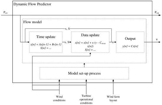
Figure 1.
System structure of a dynamic flow predictor (DFP), showing the system update process and Kalman filter time update and data update.
2.1.1. Turbine Operation Model
A static representation of the wind turbine is used and, as such, it follows turbine power set-points without delay. As shown in Figure 1, turbine power P is modeled using a direct feed-through. As such, the modeled turbine power output equals the turbine power set-point as long as the turbine power set-point is in the range of the turbine’s available power.
is the available power of a wind turbine [29], which is calculated as:
where is the air density, u the rotor effective wind speed, and the maximum power coefficient of the turbine achievable at the present wind speed. The assumption of modeling turbine power using a direct feed-through is valid if relevant turbine dynamics are either much faster or much slower than the sampling time. The sampling time used in the present work is 30 s. The relevant, in this case, fast turbine dynamics are generator power dynamics and blade pitch control dynamics, which are typically in the order of seconds. It is thus assumed that the dynamics of turbine power production can be modeled using algebraic variables.
2.1.2. Flow Model
Out of the dynamic phenomena of wind farm flow, those potentially relevant for control-oriented modeling are wake propagation, wake meandering, and turbine induction. The dynamics of induction of wind turbines settle below time spans of 10 s [30]. Given the sampling time of 30 s in this work, such dynamics are not considered in the DFP. Wake meandering is modeled in a time-averaged manner using engineering wake models [25] in the DFP. The dynamics of wake propagation are explicitly modeled in the DFP flow model. The approach of the DFP for the modeling of wake propagation, wake meandering, and turbine induction was also employed in References [25,27] and successfully validated using wind farm SCADA data and LES. In the present work, we introduce a linear version of such an approach, which is thereby well suited for linear control methods.
The flow model estimates the future wind speed at turbines that do not face upstream wake flow, using a persistence-based estimate. The aerodynamic interaction of one or multiple upstream turbines with a downstream turbine is modeled as:
where is the rotor effective wind speed of downstream turbine i at discrete time n. The rotor effective wind speed is the wind speed in the mean wind direction averaged over the rotor area of a wind turbine. All wind speeds in the present work are rotor effective wind speeds. is the wind speed at the most upstream turbine and is the wake deficit induced by upstream turbine l to downstream turbine i. is the set of all turbines upstream of turbine i. is the discrete time delay for the wake of the most upstream turbine to propagate to downstream turbine i. is the discrete time delay for the wake of upstream turbine l to propagate to downstream turbine i. The discrete time delay is defined as the integer-rounded ratio of the wake propagation delay and the sampling time as .
The duration of wake propagation can be determined in different ways, while the overall aim is to choose the model that matches the wind farm in question as close as possible. In this work, we used an engineering model [31]. In the simulation model, SimWindFarm, which is used for the testing of the DFP, the wake propagation speed is proportional to freestream flow. Thus, the model for the wake propagation delay was chosen for this work to be calculated as , where u is the measured wind speed and the distance of the propagated wake.
The wake deficit was modeled based on the Frandsen wake model [32], which estimates the wake deficit as:
where is the thrust coefficient, is the turbine’s power, and the distance from turbine l to turbine i in the mean wind flow direction. is the radius of the rotor of the upstream turbine; is the overlap area of the wake from upstream turbine l with the rotor area of downstream turbine i. is the rotor area of downstream turbine i.
The Frandsen model was chosen as the same wake deficit model is used in the simulation environment, but other wake models can be used similarly. Given the multitude of wake deficit models available in literature, the aim was generally to choose the model that matches the considered wind farm as close as possible. More details on the sensitivity of the accuracy of the DFP to the chosen wake deficit model are discussed in Section 3.2.2. The linearized wake deficit, as used in Equation (3), is modeled using the 1st order Taylor series expansion of the wake deficit model as:
where is the deviation of from the wind speed linearization point , denotes the deviation of turbine power from the power linearization point , and is the overall system linearization point. The partial derivatives of the Frandsen wake deficit model with respect to wind speed and turbine power are:
The partial derivatives of the wake deficit model (Equations (6) and (7)) are used in the linearized wake deficit model (Equation (5)), which is employed in the wake superposition model (Equation (3)). After converting the wake superposition model to state space form and joining all wake interaction processes, the total wind farm flow model can be written as:
is the wind speed delay states of all wind turbines. is the wind speed linearization point. The output of the flow model is the current rotor effective wind speed at the turbines in the wind farm. is the deviation of the turbine power set-points from the power linearization point. Matrix models the process of the wake propagation delay of all turbines and matrices , , and model the effect of wake deficit on wind flow. Matrix relates the wind speed states to the current rotor effective wind speed at the turbines in the wind farm.
In the following, the total system state space model as presented in Equation (8) is summarized as:
where is the state vector and is the control input vector. and are system process matrices and is the wind speed output matrix.
2.1.3. Kalman Filter and System Update
The process to update, the state space model is structured into three steps: (1) Time update, (2) data update, and (3) system matrix update. The first two steps constitute an ordinary Kalman filter [33]. The Kalman filter was used to improve the prediction accuracy of the DFP, by correcting the states of the flow model. A Kalman filter was chosen as it allows correcting, as shown in the Results Section, the system states using a weighted average of measurements of selected states, with more weight given to measurements with larger certainty.
Time Update
First, in the time update of the Kalman filter, the state estimate from the prior time step was used to predict the current system state at time step n based on the system model of time step . The time update is calculated as:
where is the state estimate condition to measurements up to time step . Similarly, and are system matrices at time step . The variance of the state estimate, , is updated as:
where is the covariance of the process error. The covariance is estimated using physics-based estimates of the model errors.
Data Update
Second, in the data update of the Kalman filter, the system state is updated with present system measurements, which are related to system states as:
The estimate of the measurements is wind speeds related to selected wind speed states of the flow model, such as the current rotor effective wind speed at wind turbines. Matrix relates the system states to these measurements.
The Kalman gain is calculated as:
where is the covariance of the measurement noise. The covariance is estimated using physics-based and empirical estimates of the measurement errors. The cross-correlation between and is modeled to be zero. The data update is performed as:
Matrix Update
Third, system matrices were updated based on the current system operation point. The update approach depends on the deviation of the current system state from the linearization point. If the deviation exceeds the update limit , the system matrices are updated and, as a result, the new linearization point equals the current system state. If the deviation is within the limits, the system matrices remain unchanged. Consequently, a matrix update is performed if the following condition is satisfied:
where x represents a relevant system condition, such as wind conditions and turbine operation point, and the linearization point of that condition. is the update limit. Detailed analysis of this and guidelines on choosing the appropriate update limit are discussed in Section “Computational Efficiency”.
2.2. Simulation Environment: SimWindFarm
The DFP was tested in simulations using the dynamic simulation framework SimWindFarm (SWF) [34,35].
2.2.1. Modeling Approach
SWF performs simultaneous, dynamic simulations of the wind turbines in the wind farm, the wind farm control, the aerodynamic interaction of the wind turbines, and the actions by the transmission system operator. The NREL 5 MW virtual turbine model [36] was used to model wind turbine operation. Key characteristics of the turbine model are shown in Table 1. Wind turbine aerodynamics were modeled using the turbine power coefficient and thrust coefficient [35]. Up to 3rd order, dynamic models were employed to simulate the drive train, generator, and pitch actuator. The aerodynamic model of the wind flow in the wind farm was structured into an ambient field model and a turbine wake model part. The ambient wind field was modeled as the hub height, turbulent wind flow advected with the mean wind speed under the assumption of Taylor’s frozen turbulence. Wake flow modeling includes wake wind speed deficit, wake width expansion, wake meandering, and wake merging. Wind turbines are controlled using the DTU Wind Farm Controller [37], which is linked to the SWF simulation tool and replaces the basic, standard wind farm controller in SWF.

Table 1.
Key characteristics of NREL 5 MW turbine model used in all SimWindFarm (SWF) simulations.
2.2.2. Validity as Test Environment
The use of engineering models for the modeling of the dynamics of wind farm flow was successfully validated in References [25,27], as discussed in Section 2.1.2 “Flow Model”. The validation of the DFP therefore aimed to investigate how well the linearized engineering model of the DFP compares to the nonlinear engineering models of the higher-fidelity SWF. The flow model in SWF is more complex. It includes the effects of wake meandering, nonlinear, multiple wake modeling and wake merging, which are not all considered in the DFP. The main similarity between the DFP and SWF is the wake deficit model. Section 3.2.2 evaluates the effect of using a different deficit model in the DFP. The results showed that the modeling approach of the DFP is valid with the use of different deficit models. Second, SWF models a variety of turbine dynamics with up to 3rd order dynamic equations, whilst no turbine dynamics are modeled in the DFP.
2.2.3. Simulation Conditions
All SWF simulations were performed in the same wind conditions. The simulated wind conditions had a mean wind speed of 8 m/s and a turbulence intensity of 6%. The wind direction was considered aligned with the turbine row, if not indicated differently in the discussion.
3. Results and Discussion
The DFP was tested on a two-turbine array to illustrate its main characteristics and a large-scale wind farm to showcase its application in a realistic configuration.
3.1. Two-Turbine Case Study
In the two-turbine case study, the effect of Kalman filtering and wind direction on the performance of the DFP were investigated and the computational efficiency of the DFP is discussed. A two-turbine wind farm was chosen as it is the simplest set-up possible to analyze these effects and thereby eases the understanding of the work. In the following, first, the simulation set-up is introduced and second, the case study results are presented.
3.1.1. Simulation Set-Up
The case study was performed in the dynamic simulation tool SWF. The employed wind farm layout and wind farm operation mode are discussed in more detail in the following.
Wind Farm Layout
The layout of the simulated two-turbine array is shown in Figure 2. As such turbine No. 1 is the upstream turbine and turbine No. 2 the downstream turbine. The turbine array was spaced with 4.3 rotor diameters (D).
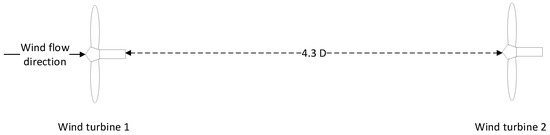
Figure 2.
Layout of two-turbine array used for the testing of DFP.
Wind Farm Operation
In all the simulations in this study, the wind farm was operated in the ancillary service “active power constraint mode” [38]. Both case studies used the same normalized total power reference signal of the “active power constraint mode”. The total power reference signal was further chosen so that the resulting individual turbine power references would never exceed a turbine’s available power in either of the case studies.
Figure 3a shows the simulated total farm power output, the total power reference signal, and the wind farm available power for the two-turbine case study. The power was normalized with the rated wind farm power. The wind farm was controlled using the DTU Wind Farm Controller’s closed-loop PI-controller with the equal dispatch function [9] in both case studies. It can be observed that the total farm power follows the total power reference well. The normalized root-mean-square deviation from the reference is 0.35%. The wind turbines were controlled using a standard wind turbine control approach [4]. The reduction of the turbines’ power below the available power resulted in the turbines operating at the rated rotor rotational speed while controlling aerodynamic power using the pitch controller. Figure 3b. shows the dynamics of the blade pitch angle of the wind turbines. The observed variation of the pitch angle resulted in a variation of the turbine’s thrust and consequently, also in a variation of the wake deficit generated by that turbine.
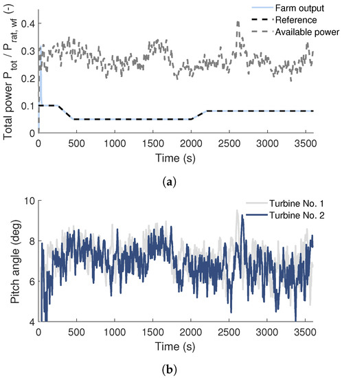
Figure 3.
Simulated operation of two-turbine array used for comparison with DFP. Shown are (a) total farm power and (b) blade pitch angle.
3.1.2. Results
The benefits of the Kalman filter, the computational efficiency of the DFP, and the effect of wind direction on the performance of the DFP are discussed in the following.
Benefits of Kalman Filtering
Tests of the DFP showed that the use of the Kalman filter can significantly improve the accuracy of wind speed prediction. Figure 4 shows a comparison of the wind speed estimate of the DFP with the test environment SWF. The wind speed is compared at the location of the two turbines. Figure 4a shows the wind speed at upstream turbine No. 1. It can be observed that the wind speed prediction by the DFP is in good agreement with SWF. The normalized root-mean-square (RMS) deviation of the wind speed prediction of the DFP is 4.8%, both with and without the use of the Kalman filter. It is evident that there is a time lag of one time step in the wind speed estimates of the DFP, both with and without the use of the Kalman filter. This is due to the definition of the wind speed state in the DFP. The wind speed state at a time step n is defined as the mean wind speed over the time interval . The wind speed at the upstream turbine at time step n is calculated using a persistence-based prediction from the wind speed measurements over the time interval . As a result, the DFP wind speed estimate at the upstream turbine has a lag of one time step.
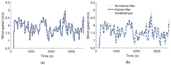
Figure 4.
Sampled rotor effective wind speed simulated using SWF and predicted using DFP with and without use of Kalman filter. Shown are wind speeds of (a) turbine No. 1 and (b) turbine No. 2.
Figure 4b shows the wind speed at downstream turbine No. 2. It can be observed that the DFP predictions of wind speed are in good agreement with SWF. The normalized RMS prediction error is 4.4% without the use of the Kalman filter. The use of the Kalman filter reduces the error by 70% to a RMS error of only 1.3%, as shown in Figure 5. The error reduction is achieved as the Kalman filter allows to correct both measurable and not measurable states of the DFP model.
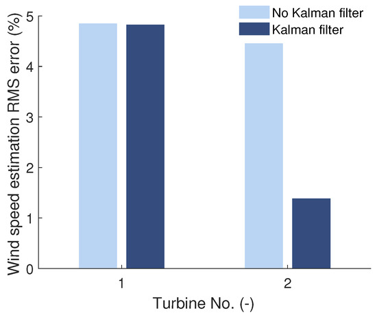
Figure 5.
Root-mean-square (RMS) deviation of rotor effective wind speed estimation at turbines of two-turbine array. RMS deviation is normalized with mean freestream wind speed.
Computational Efficiency
Model-based control benefits from computationally fast models. Since the DFP was developed for use in model-based control, computational effectiveness is a core characteristic. Low computational cost is achieved by the use of the dynamic model update and the low computation time required for an iteration of the state space system of the DFP. The computation time per iteration is discussed in the large-scale wind farm case study in Section 3.2, since it is a computationally demanding scenario. The benefit of the dynamic model update is discussed on the two-turbine array in the following, as the simpler set-up eases the understanding.
The dynamic model update decides dynamically on executing updates, as described in Section “Matrix Update”. It thereby aims to reduce computational cost by decreasing the frequency of model updates, while retaining the accuracy of the DFP. The approach is to perform a model update only when the deviation of the system operation point from the linearization point exceeds the user-defined update limit . With larger deviations from the linearization point, the difference between the linear model and the real system increases. Hence, it is the aim to choose the update limit so that deviations from the operation point are small and the linear model remains representative of the behavior of the real system.
The impact of the operational conditions on the update frequency and accuracy of the model is discussed in the following. First, a wide range of wind turbine downregulation is investigated in a simulation study. The study also covers the effect of turbulent wind speed. Thereafter, the impact of other variations of wind conditions are discussed. The study is conducted in two scenarios of wind farm operation and thereby covers a wide range of downregulation. In both scenarios, the two-turbine array is operated in the “active power constraint mode” [38], that is, a total power of 1.8 MW in scenario 1 and 0.9 MW in scenario 2, as shown in Figure 6a. Albeit the total power of the wind farm and the turbine power is constant in the simulation, the turbulent wind speed results in a variation of the turbines’ power coefficient, as depicted in Figure 6b. The wind field and the wind farm layout are the same as for the other investigations of the two-turbine case study.
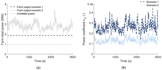
Figure 6.
Wind farm in two operation scenarios used for demonstration of effect of update limit on model update frequency, model accuracy and computational cost. Shown are (a) total power of wind farm and (b) power coefficient at upstream turbine.
Figure 7 shows the effect of the update limit on model update frequency and model accuracy for both operation scenarios. The accuracy is the RMS error of rotor effective wind speed at downstream turbine No. 2. The error in estimating the wind speed at the upstream turbine is not part of this analysis, since it is not affected by the matrix update. Update frequency is defined as the average ratio of matrix updates to model iterations . The study is performed without the use of the Kalman filter, so the estimation accuracy is only dependent on the linearization approach.
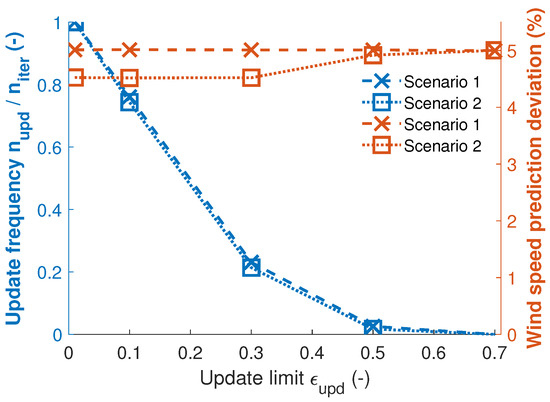
Figure 7.
Impact of matrix update limit on downstream turbine wind speed prediction accuracy (right) and matrix update frequency (left).
It can be observed that in scenario 1, the model accuracy is insensitive to the update frequency. In scenario 2, the model accuracy is constant up to an update limit of 0.3. Increasing the update limit from 0.3 to 0.5 results in an increase of model error from 4.5% to 4.9%. Hence, the choice of an update limit of 0.25 for the other investigations of this work, as described in Section “Matrix Update”, appears to be sufficient to retain accuracy. The results also showed that the update frequency can be reduced by 100% in scenario 1 and by 97% in scenario 2 without compromising model accuracy.
Generally, the extent to which the update limit can be increased without compromising accuracy depends on the operating conditions, that is, the operation point and the dynamic behavior of the system around it. The dominant dynamics in the present study are variations of wind speed and turbine operation point, illustrated by the power coefficient, as shown in Figure 6b. In scenario 1, the power coefficient of the upstream turbine is 0.26 on average and varies with a standard deviation of 18%. In scenario 2, the power coefficient of the upstream turbine is 0.13 on average and varies with a standard deviation of 18%. The power coefficients covered in both scenarios range from 0.07 up to 0.45. As the maximum power coefficient is 0.48, a wide range of turbine downregulation levels is covered by the two scenarios.
The results showed that for the dynamic conditions of the present study, only few model updates were required to retain model accuracy. It is of interest to understand how other variations of operational conditions relevant for power control of wind farms impact update frequency. Such variations are changes of turbulence intensity and of the 10min-average wind speed and wind direction, which could be shifts in the order of 1%, 1 m/s and 5, respectively. Since these changes typically occur at time scales in the order of several minutes, their impact on the update frequency will not be significant. The changes of atmospheric boundary layer conditions typically occur at even larger time scales and are therefore also not having a significant impact on update frequency.
Effect of Wind Direction
The impact of the full range of wind directions and wake situations on the accuracy of the DFP is investigated in the following. Figure 8 shows the effect of the alignment of the two-turbine array with the mean wind direction on the accuracy of the DFP. In the study, the Kalman filter of the DFP is active. In Figure 8a, it can be observed that the accuracy at both turbines varies with wind direction. The variation at the upstream turbine is because the wind fields differ between the simulations of different wind directions. Each wind field is based on a distinct turbulence seed and as a result, the turbulence intensity varies between the wind fields. It can be shown that this difference in turbulence intensity results in the observed variation of the error of the persistence-based prediction at the upstream turbine.
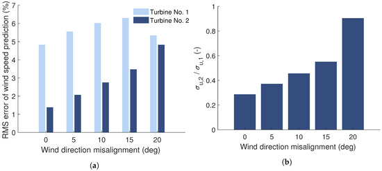
Figure 8.
Effect of alignment of turbine array with wind direction on accuracy of estimation of rotor effective wind speed. Shown are (a) accuracy for each turbine and (b) ratio of RMS wind speed estimation error at downstream turbine to RMS wind speed estimation error at upstream turbine.
The turbulence intensity-driven variation of the error in the prediction of wind speed at the upstream turbine propagates into the error in the prediction of wind speed at the downstream turbine. To remove this effect and allow to focus on the impact of wind direction, Figure 8b shows the ratio of these errors. As such, the RMS error for the downstream turbine is normalized by the RMS error for the upstream turbine. It can be observed that the accuracy of wind speed prediction for the downstream turbine decreases with an increase in wind direction misalignment. With larger misalignment, the correlation of the wind speed of the two turbines decreases and, thus, results in an increasing error of the model. Nonetheless, the error at the downstream turbine is smaller than the persistence-based prediction error at the upstream turbine. At 20° misalignment, the wake from the upstream turbine is not affecting the downstream turbine. Hence, the wind speed estimate at turbine No. 2 is also a persistence-based wind speed estimate. Since both turbines use persistence-based estimates, the ensemble average of the wind speed estimation error is expected to be the same at both turbines. The observed higher prediction accuracy at the downstream turbine is likely to be due to the seed of the turbulent wind field in SWF.
To conclude the two-turbine case study, the above investigations show the benefit of the Kalman filter and the dynamic model update, and the suitability of the DFP for different wake situations.
3.2. Large-Scale Wind Farm Case Study
In the large-scale wind farm case study, the performance of the DFP was demonstrated in key areas relevant to the model’s application to large wind farms. The model’s performance was analyzed with respect to its accuracy in the prediction of wind speed and available turbine power. Additionally, the sensitivity of the accuracy of the DFP with respect to the employed wake deficit model is discussed. The layout of the wind farm is depicted in Figure 9. The spacing of the wind turbines is five rotor diameters between both rows and columns of the square-grid wind farm layout. The wind farm comprises 80 NREL 5 MW wind turbines [36].
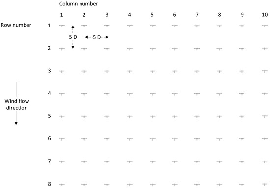
Figure 9.
Layout of large-scale wind farm used for the testing of DFP.
3.2.1. Benefit of Kalman Filter
Figure 10 shows the accuracy of the DFP in estimating the wind speed at the turbines of the large-scale wind farm. The accuracy is quantified as the normalized RMS difference between the wind speed estimated by the DFP and SWF. Figure 10a provides an overview of the variation of the accuracy across the wind turbines of the wind farm. The results were obtained with the use of the Kalman filter. It can be observed that the accuracy varies between an error of 0.8% and 4.1% at downstream turbines. Along turbine rows, the accuracy is similar. This is because the only differences between turbine columns are stochastic differences in the wind field. As a result, the standard deviation of the error within a row is less than 0.5%. The variation of accuracy along turbine columns is larger than along turbine rows. Along columns, the accuracy varies due to the difference in the wake deficit summation approach that is employed in the DFP and SimWindFarm.
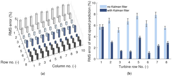
Figure 10.
Accuracy of DFP in estimation of current rotor effective wind speed at turbines of large-scale wind farm. Accuracy is quantified as normalized RMS error of wind speed estimated using DFP given SWF as reference. Shown are (a) distribution of accuracy across turbines in wind farm with DFP using Kalman filter, and (b) effect of Kalman filter on row-wise accuracy statistics, that is, mean error (bars) and standard deviation of error (errorbars).
Figure 10b shows the effect of the Kalman filter on the row-wise error statistics. The accuracy is quantified as the normalized RMS difference between the wind speed estimated by the DFP and SWF. It is observed that the use of the Kalman filter improved accuracy, on average, by 57%. The improvement in accuracy varies across turbines. A variation of the improvement in accuracy obtained by the use of the Kalman filter is also reported in Reference [27]. Like in the present paper, the work used the Kalman filter to correct an engineering model-based, dynamic model of wind farm flow.
3.2.2. Sensitivity of Wake Model
An important aspect of the DFP is the wake deficit model. Thus, it is of interest to investigate the sensitivity of the accuracy of the DFP to the employed wake deficit model. A comparison was conducted between the use of the Frandsen model, that is, the model used for all other studies in this work, and the use of the Jensen model [39]. The wake deficit model employed in SWF remains unchanged, i.e., the Frandsen model. Figure 11 shows the row-wise statistics of the error in wind speed prediction of the DFP for these two cases.
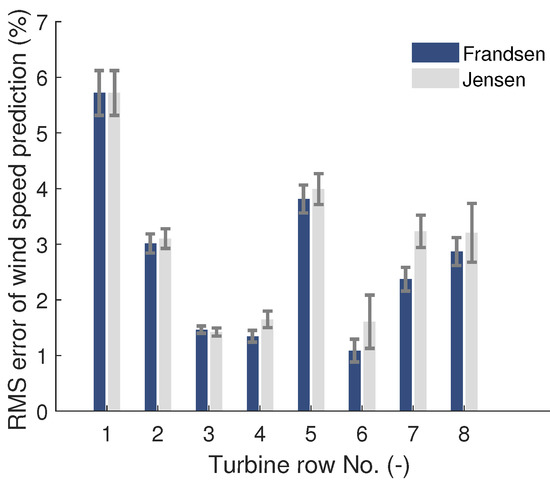
Figure 11.
Effect of wake deficit model on error of DFP in estimation of current rotor effective wind speed at turbines of large-scale wind farm. Shown are the row-wise statistics, that is, mean (bars) and standard deviation (errorbars) of the normalized RMS difference of wind speed between the DFP and SWF.
It can be observed that the use of the Jensen model increased the error at further downstream turbines. Yet, despite the larger uncertainty in the wake deficit model, the error of the DFP remained in the same range as with the Frandsen model, that is, below 4.5%. The results thus show that the DFP can provide accurate wind speed estimates even with larger uncertainty in the wake deficit model.
3.2.3. Wind Speed Prediction
The prediction of wind speed at wind turbines over time horizons in the order of minutes is useful for wind farm control. The analysis of the model’s capability for future wind speed prediction showed that the DFP can provide wind speed predictions with an error of less than 4% over a time horizon of up to 5 min. The reference to the DFP predictions is SWF. Figure 12 shows the row-averaged accuracy of the ten-step-ahead prediction of wind speed at the turbines of the large-scale wind farm. Wind speed predictions were calculated using the state space-driven prediction approach employed in model predictive control. The accuracy was quantified using the RMS difference between the DFP predictions and SWF from 126 predictions. The results were obtained with the use of the Kalman filter.
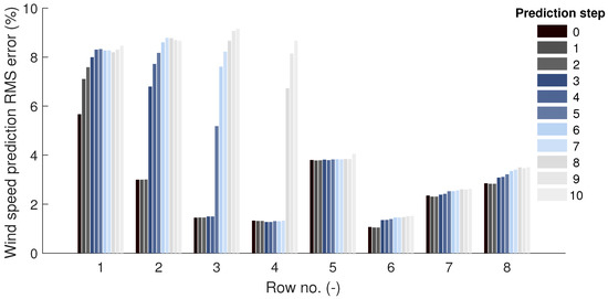
Figure 12.
Accuracy of 10-step ahead prediction of rotor effective wind speed at rows of large-scale wind farm. Accuracy is normalized RMS difference between DFP prediction and SWF flow model averaged over turbine rows. Kalman filter in DFP is active.
It can be observed that the low error obtained for prediction step 0 can be sustained over several steps into the future, with more steps at further downstream turbines. After several prediction steps, the error raises to a higher level. This can be seen, for example, in Figure 12 at turbine No. 4 from prediction step 7 to prediction step 8. The number of steps with low error equals the number of the model’s internal delay states. Further downstream turbines have a longer accurate prediction horizon due to the larger number of internal delay states. Predictions beyond the model’s internal delay states are based on persistence and, thus, less accurate. Future work will focus on extending the length of the accurate prediction horizon by exchanging the persistence-based wind speed estimate at the upstream turbine with an individual turbine-focused prediction method, such as a statistical model, as used in Reference [15].
3.2.4. Available Power Prediction
The prediction of the turbines’ available power is needed for wind farm control. Figure 13 shows the row-averaged RMS error in the prediction of the available power of the turbines of the large-scale wind farm. The available power is calculated using Equation (2) and the wind speed predictions of the DFP, as described in Section 3.2.3 above. As expected, it can be observed that the pattern in the error of available power prediction is the same as for the analysis of wind speed prediction discussed with Figure 12. The error in the prediction of turbine available power ranges between 1.5% to 14%, considering predictions based on the model’s internal delay states only.
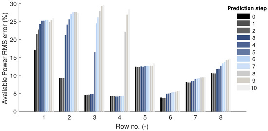
Figure 13.
Accuracy of 10-step ahead prediction of turbine available power for each row of large-scale wind farm. Accuracy is normalized RMS difference between DFP prediction and SWF averaged over turbine rows. Kalman filter in DFP is active.
3.2.5. Computation Time
As described in Section “Computational Efficiency”, model-based control benefits from the low computation time required per iteration of the state space system of the DFP. To provide a ’worst-case’ estimate, the computation time was quantified for the computationally-challenging, realistic-scale 80-turbine wind farm. The calculations were performed on a standard personal computer in MATLAB. The available hardware of the computer are one core of a 2.6 GHz processor and 8GB installed memory. On average, the computation time per iteration of the state space system was s.
4. Conclusions
This work introduces the DFP, a control-oriented, linear dynamic wind farm flow and operation model suited for model predictive control of wind farms. The results of this work showed the suitability, accuracy, and computational speed of the modeling approach of the DFP. Suitability was proven since the DFP can accurately capture the dynamics of wind farm flow in SWF, even for complex wind farm configurations. Furthermore, it is demonstrated in the literature that engineering models, such as those used in the DFP, are suited for the prediction of the dynamics of wind farm flow. Accuracy was demonstrated in the control-relevant prediction of wind speed and turbine available power. In the large-scale wind farm case study, the Kalman filter of the DFP reduced the error in wind speed prediction, on average, by 57%. As a result, current wind speed was estimated with a RMS error ranging between 0.8% and 4.1%. The error of wind speed predictions was less than 4% for a time horizon of 5 min. For the same horizon, turbine available power was predicted with an error ranging between 1.5% and 14%. Beneficial for the computational speed of the DFP is the use of a dynamic model update and the low computation time per state space system iteration. For the investigated, realistic-scale, 80 turbine wind farm, the computation time per iteration was, on average, s. Based on the results presented, we think that the DFP model represents a viable solution for moving wind farm control philosophy towards linear control approaches.
Author Contributions
Conceptualization, J.K. and N.A.C.; Methodology, J.K. and N.A.C.; Software, J.K.; Validation, J.K.; Formal Analysis, J.K.; Investigation, J.K.; Resources, N.A.C.; Data Curation, J.K.; Writing—Original Draft Preparation, J.K.; Writing—Review and Editing, N.A.C.; Visualization, J.K.; Supervision, N.A.C.; Project Administration, N.A.C.; Funding Acquisition, N.A.C.
Funding
This research was funded by the CONCERT project, which is funded by Energinet.dk under the Public Service Obligation scheme (ForskEL 12396) with project partners Vattenfall R&D and Siemens Wind Power.
Acknowledgments
Vattenfall R&D and Siemens Wind Power are gratefully acknowledged for the fruitful discussions during the development of the DFP approach.
Conflicts of Interest
There are no competing interests.
Abbreviations
The following abbreviations are used in this manuscript:
| CFD | Computational fluid dynamics |
| DFP | Dynamic Flow Predictor |
| DTU | Technical University of Denmark |
| RMS | Root-mean-square |
| SWF | SimWindFarm |
References
- Global Wind Energy Council (GWEC). Global Wind Report 2017. Available online: http://gwec.net/ (accessed on 19 November 2018).
- Fernandez-Gamiz, U.; Zulueta, E.; Boyano, A.; Ansoategui, I.; Uriarte, I. Five megawatt wind turbine power output improvements by passive flow control devices. Energies 2017, 10, 742. [Google Scholar] [CrossRef]
- Hansen, M.O.; Sørensen, J.N.; Voutsinas, S.; Sørensen, N.; Madsen, H.A. State of the art in wind turbine aerodynamics and aeroelasticity. Prog. Aerosp. Sci. 2006, 42, 285–330. [Google Scholar] [CrossRef]
- Pao, L.Y.; Johnson, K.E. A tutorial on the dynamics and control of wind turbines and wind farms. In Proceedings of the 2009 American Control Conference, St. Louis, MO, USA, 10–12 June 2009; pp. 2076–2089. [Google Scholar] [CrossRef]
- Kazda, J.; Zendehbad, M.; Jafari, S.; Chokani, N.; Abhari, R.S. Mitigating adverse wake effects in a wind farm using non-optimum operational conditions. J. Wind Eng. Ind. Aerodyn. 2016, 154, 76–83. [Google Scholar] [CrossRef]
- Annoni, J.; Gebraad, P.M.; Scholbrock, A.K.; Fleming, P.A.; Wingerden, J.W.V. Analysis of axial-induction-based wind plant control using an engineering and a high-order wind plant model. Wind Energy 2016, 19, 1135–1150. [Google Scholar] [CrossRef]
- Hansen, A.D.; Sørensen, P.; Iov, F.; Blaabjerg, F. Centralised power control of wind farm with doubly fed induction generators. Renew. Energy 2006, 31, 935–951. [Google Scholar] [CrossRef]
- Van Wingerden, J.W.; Pao, L.; Aho, J.; Fleming, P. Active power control of waked wind farms. IFAC-PapersOnLine 2017, 50, 4484–4491. [Google Scholar] [CrossRef]
- Kazda, J.; Merz, K.; Tande, J.O.; Cutululis, N.A. Mitigating turbine mechanical loads using engineering model predictive wind farm controller. J. Phys. Conf. Ser. 2018, 1104, 012036. [Google Scholar] [CrossRef]
- Soleimanzadeh, M.; Wisniewski, R.; Kanev, S. An optimization framework for load and power distribution in wind farms. J. Wind Eng. Ind. Aerodyn. 2012, 107–108, 256–262. [Google Scholar] [CrossRef]
- Horvat, T.; Spudic, V.; Baotic, M. Quasi-stationary optimal control for wind farm with closely spaced turbines. In Proceedings of the 35th International Convention MIPRO, Opatija, Croatia, 21–25 May 2012; pp. 829–834. [Google Scholar]
- Gebraad, P.M.O.; Teeuwisse, F.W.; van Wingerden, J.W.; Fleming, P.A.; Ruben, S.D.; Marden, J.R.; Pao, L.Y. Wind plant power optimization through yaw control using a parametric model for wake effects—A CFD simulation study. Wind Energy 2016, 19, 95–114. [Google Scholar] [CrossRef]
- Kazda, J.; Göçmen, T.; Giebel, G.; Cutululis, N. Possible improvements for present wind farm models used in optimal wind farm controllers. In Proceedings of the 15th International Workshop on Large-Scale Integration of Wind Power into Power Systems as well as on Transmission Networks for Offshore Wind Power Plants, Vienna, Austria, 15–17 November 2016. [Google Scholar]
- Crespo, A.; Hernández, J. Turbulence characteristics in wind-turbine wakes. J. Wind Eng. Ind. Aerodyn. 1996, 61, 71–85. [Google Scholar] [CrossRef]
- Riverso, S.; Mancini, S.; Sarzo, F.; Ferrari-Trecate, G. Model predictive controllers for reduction of mechanical fatigue in wind farms. IEEE Trans. Control Syst. Technol. 2017, 25, 535–549. [Google Scholar] [CrossRef]
- Mikkelsen, T.; Angelou, N.; Hansen, K.; Sjoholm, M.; Harris, M.; Slinger, C.; Hadley, P.; Scullion, R.; Ellis, G.; Vives, G. A Spinner-integrated wind lidar for enhanced wind turbine control. Wind Energy 2013, 16, 625–643. [Google Scholar] [CrossRef]
- Schlipf, D.; Schlipf, D.J.; Kühn, M. Nonlinear model predictive control of wind turbines using LIDAR. Wind Energy 2013, 16, 1107–1129. [Google Scholar] [CrossRef]
- Boersma, S.; Gebraad, P.; Vali, M.; Doekemeijer, B.; van Wingerden, J. A control-oriented dynamic wind farm flow model: “WFSim”. J. Phys. Conf. Ser. 2016, 753, 032005. [Google Scholar] [CrossRef]
- Soleimanzadeh, M.; Wisniewski, R.; Brand, A. State-space representation of the wind flow model in wind farms. Wind Energy 2014, 17, 627–639. [Google Scholar] [CrossRef]
- Knudsen, T.; Bak, T.; Soltani, M. Prediction models for wind speed at turbine locations in a wind farm. Wind Energy 2011, 14, 877–894. [Google Scholar] [CrossRef]
- Wang, J.; Hu, J. A robust combination approach for short-term wind speed forecasting and analysis—Combination of the ARIMA (Autoregressive Integrated Moving Average), ELM (Extreme Learning Machine), SVM (Support Vector Machine) and LSSVM (Least Square SVM) Forecasts Using a GPR (Gaussian Process Regression) Model. Energy 2015, 93, 41–56. [Google Scholar] [CrossRef]
- Jung, J.; Broadwater, R.P. Current status and future advances for wind speed and power forecasting. Renew. Sustain. Energy Rev. 2014, 31, 762–777. [Google Scholar] [CrossRef]
- Shapiro, C.R.; Meyers, J.; Meneveau, C.; Gayme, D.F. Wind farms providing secondary frequency regulation: evaluating the performance of model-based receding horizon control. Wind Energy Sci. 2018, 3, 11–24. [Google Scholar] [CrossRef]
- Gebraad, P.M.O.; van Wingerden, J.W. A Control-oriented dynamic model for wakes in wind plants. J. Phys. Conf. Ser. 2014, 524, 012186. [Google Scholar] [CrossRef]
- Gogmen, T.; Giebel, G.; Poulsen, N.K.; Sørensen, P.E. Possible power of down-regulated offshore wind power plants: The PossPOW algorithm. Wind Energy 2018. [Google Scholar] [CrossRef]
- Boersma, S.; Doekemeijer, B.; Vali, M.; Meyers, J.; Wingerden, J.w.V. A Control-oriented dynamic wind farm model: WFSim. Wind Energy Sci. 2018, 3, 75. [Google Scholar] [CrossRef]
- Gebraad, P.M.O.; Fleming, P.A.; Van Wingerden, J.W. Wind turbine wake estimation and control using FLORIDyn, a control-oriented dynamic wind plant model. In Proceedings of the American Control Conference, Chicago, IL, USA, 1–3 July 2015; pp. 1702–1708. [Google Scholar] [CrossRef]
- Bay, C.J.; Annoni, J.; Taylor, T.; Pao, L.; Johnson, K. Active power control for wind farms using distributed model predictive control and nearest neighbor communication. In Proceedings of the Annual American Control Conference, Milwaukee, WI, USA, 27–29 June 2018; pp. 682–687. [Google Scholar] [CrossRef]
- Göçmen, T.; Giebel, G.; Sørensen, P.E.; Poulsen, N.K. Possible Power Estimation of Down-Regulated Offshore Wind Power Plants. Ph.D. Thesis, Technical University of Denmark (DTU), Kongens Lyngby, Denmark, 2016. [Google Scholar]
- Øye, S. Tjæreborg Wind Turbine (Esbjerg): First Dynamic Inflow Measurement; Technical Report; DTU Wind Energy: Roskilde, Denmark, 1991. [Google Scholar]
- Machefaux, E.; Larsen, G.C.; Troldborg, N.; Gaunaa, M.; Rettenmeier, A. Empirical modeling of single-wake advection and expansion using full-scale pulsed lidar-based measurements. Wind Energy 2015, 18, 2085–2103. [Google Scholar] [CrossRef]
- Frandsen, S.; Barthelmie, R.; Pryor, S.; Rathmann, O.; Larsen, S.; Hojstrup, J. Analytical modelling of wind speed deficit in large offshore wind farms. Wind Energy 2006, 9, 39–53. [Google Scholar] [CrossRef]
- Kalman, R.E.; Bucy, R.S. New results in linear filtering and prediction theory. J. Basic Eng. 1961, 83, 95. [Google Scholar] [CrossRef]
- Grunnet, J.; Soltani, M.; Knudsen, T. Aeolus toolbox for dynamics wind farm model, simulation and control. In Proceedings of the European Wind Energy Conference & Exhibition (EWEC 2010), Warszawa, Poland, 20–23 April 2010; pp. 3119–3129. [Google Scholar]
- Grunnet, J.; Soltani, M.; Knudsen, T. SimWindFarm Official Website. 2016. Available online: http://www.ict-aeolus.eu/SimWindFarm/ (accessed on 19 November 2018).
- Jonkman, J.; Butterfield, S.; Musial, W.; Scott, G. Definition of a 5-MW Reference Wind Turbine for Offshore System Development; Technical Report No. NREL/TP-500-38060; National Renewable Energy Laboratory: Golden, CO, USA, 2009. [Google Scholar]
- Kazda, J.; Göçmen, T.; Giebel, G.; Courtney, M.; Cutululis, N. Framework of multi-objective wind farm controller applicable to real wind farms. In Proceedings of the WindEurope Summit 2016, Hamburg, Germany, 27–29 September 2016. [Google Scholar]
- Energinet.dk. Technical Regulation for Wind Power Plants with a Power Output Above 11 kW. Available online: http://osp.energinet.dk/ (accessed on 19 November 2018).
- Jensen, N.O. A Note on Wind Generator Interaction; Risø National Laboratory: Roskilde, Denmark, 1983. [Google Scholar]
© 2018 by the authors. Licensee MDPI, Basel, Switzerland. This article is an open access article distributed under the terms and conditions of the Creative Commons Attribution (CC BY) license (http://creativecommons.org/licenses/by/4.0/).