1. Introduction
Presently, the aging power grid infrastructure is now gradually improving due to the emerging technological innovations. This improvement witnessed by the recent innovations does not only revive the interest of researchers and socio-economic development. However, it has a great benefit to the society at large. Despite this improvement, the majority of power generation relied on the conventional electric power distribution network. This network is very complicated and cannot meet the demands of the 21st century [
1]. More so, this intricate network is influenced by the following factors. Firstly, the growing population, global climatic change, equipment malfunction and exponential demands for electricity. Lastly, the electric storage problems, strength of the generating plants, one-way communication, resilience problem and the shortage of fossil fuel. To address the above limitations, the concept of smart grid (SG) is adopted to include the renewable energy sources (RES) [
2]. The advent of SG is not only beneficial to all those involved in the electric power industry. However, it has numerous stakeholders.
To actualize the capabilities of SG, the demand side management (DSM) is included in the existing SG, since it provides alteration in the consumer demand for electricity. This can be achieved through several methods like financial incentives and behavioral change via education. Generally, the aim of DSM is to motivate consumers to reduce their electricity consumption during peak hours as well as in critical periods. DSM uses demand response (DR) which plays a significant role in the operation of the power grid by shifting the electricity usage during the peak period in response to the market prices. This also involves other forms of financial incentives as well as balancing supply and demand.
To efficiently implement the DSM strategies, home energy management system (HEMS) is used to minimize the generation cost of electricity by shifting certain household loads to off-peak hours. This can be done by optimally adjusting the energy obtained from the power grid. HEMS involves scheduling of certain household loads that have high priority as they are important for meeting the consumer’s satisfaction. Thus, the request of such loads has to be met instantly and the energy minimization potency of such loads is not easily rescheduled. However, such loads can be combined with RES and energy storage system (ESS) for which peak hour consumption is minimized. Nevertheless, some loads can be rescheduled to the period of low consumption. Scheduling periods are determined by the consumers’ choice settings. In this paper, we describe such household loads as shiftable appliances. On the contrary, some household loads have controllable patterns. Hence, the electricity cost can be minimized based on the electricity consumption profile of such loads.
Reliable operations of HEMS require coordination among the ESS and loads which can be achieved through different optimization techniques. These techniques are of two types. The traditional techniques require the exact rules for changing one solution into another. It is fundamentally deterministic in nature and has shown tremendous achievement in the field of science and engineering. Examples of these optimization techniques are dynamic programming, generalized reduced gradient method, nonlinear and linear programming, and quadratic and geometric programming [
3,
4,
5,
6]. Other optimization techniques are meta-heuristic with an inherent probabilistic transformation rules [
7,
8,
9,
10].
The commonly used heuristic optimization algorithms can be evolutionary or iterative based methods. However, as the number of optimization variables increases, the computational complexities increase as well, especially with iterative methods. On the contrary, it is not with the case of evolutionary methods. However, evolutionary methods are faced with local optimum problem. Examples of heuristic algorithms are either swarm intelligence-based, biological-inspired, nature-inspired, population-based or musical-inspired phenomena. These heuristic optimization algorithms are stochastic with common controlling parameters like generation size, elite size, and population size while others have algorithmic specific control parameters [
11]. The best possible adjustment of these algorithmic specific control parameters is the essential factor that can influence algorithm’s performance. This adjustment avoids high computational complexity and prevents yielding a local optimum solution.
Several pricing schemes are now introduced by utility to calculate the electricity tariffs of different periods of the day. This is done to reshape the consumer consumption patterns. Some electricity tariffs are computed on an hourly or day-ahead basis, whereas a day is divided into periods such as off-peak, mid peaks and on-peak hours, and the electricity tariff is calculated for such periods. During critical events or hours, consumers are charged with peak rate that is higher than any other rate.
This paper is the extension of work in [
12] which includes shared RES and ESS to supply energy to multiple residential households. For the load scheduling, an Earliglow based optimization algorithm is proposed to shift loads within the time-of-use (ToU) and critical peak pricing (CPP) scheduling horizon for 24 h. The Earliglow algorithm has both flavors of the existing techniques, Jaya and strawberry algorithm (SBA). The proposed algorithm reduces the number of iterations created by SBA since SBA duplicates every computational individual at each iteration as well as local and global search problem. Furthermore, the proposed algorithm ensures that the solution moves towards the ideal solution by circumventing the worse solution. The proposed algorithm becomes efficient, if the best optimal solution is obtained. In addition, a battery is considered for energy storage and it gets charged only if the energy produced by the RES is greater than the load demands. Otherwise, the battery will be discharging. The state of charge (SOC) of the battery depends on the history of battery and the differences between the power generated by RES and the load demands.
This paper is organized as follows:
Section 2 presents the related work. Afterwards,
Section 3 includes the problem statement and the system model description. In
Section 4, the proposed model is given in detail. Next, simulation results and discussions, and the feasible region (FR) is discussed in
Section 5. Finally,
Section 6 concludes the work with future work.
2. Related Work
The implementation of heuristic optimization algorithm has been proposed in order to derive solutions within a reasonable amount of execution time. Because of its ability to handle complex problems of nonlinear nature, extra decision variables can be included without increasing the execution time. However, considering the stated pros, there is the need for dynamic and deterministic algorithms to provide an accurate optimal solution to home energy management (HEM) scheduling problems.
Maytham et al. [
3] propose a real optimal controller for HEMS using new binary backtracking search algorithm (BBSA). The proposed controller reduces the energy consumption and electricity cost, and ensures energy savings at peak hours for weekdays and weekends. The proposed algorithm is compared with binary particle swarm optimization (BPSO) to ascertain the accuracy of their proposed controller in the HEMS. Within household surroundings, smart meters coordinate with both real time and appliances scheduling via HEMS. Abdul et al. [
4] propose an autonomous energy management system, which is formulated by the mixed integer linear programming (MILP) and the Dijkstra algorithm for reducing the electricity cost of the real time load. An efficient solution is obtained with lower complexity via the proposed HEMS without disturbing the operation of non shiftable appliances.
Energy monitoring plays a vital role in energy management. As such, it is required to monitor the energy consumption of household devices before commencing on the technical measures to reduce energy consumption. Abubakar et al. [
5] demonstrate energy management via intrusive load monitoring (ILM) and non-intrusive load monitoring (NILM). The proposed techniques reduce electricity cost, provide cost savings and minimize the greenhouse emission. Addressing the challenges involving high dimensional optimization problems for iterative HEM, Hepeng et al. [
6] propose an approximate dynamic programming (ADP). It is used as the mechanism for energy management of vehicle-to home (V2home) and vehicle-to grid (V2grid). Due to the large number of DR capable devices, the proposed method is useful for minimizing the energy cost and providing peak load shifting for the iterative HEM.
Currently, DSM schemes have been proposed for residential, commercial and industrial sectors. These schemes are useful in reducing the energy profile of consumers in the grid area network. In this respect, work in [
9] implements a hybrid genetic wind-driven optimization (GWD) technique for scheduling the residential household loads. The GWD technique is able to shift the load in a real-time pricing (RTP) environment between on-peak and off-peak hours. In addition, it reduces electricity cost and the consumer’s comfort is protected. In order to show a higher search efficiency and dynamic capability to achieve an optimal solution, Hafiz et al. [
13] present an efficient HEMS (EHEMS) based on a genetic harmony search algorithm (GHSA). This proposed method reduces the electricity cost, peak-to-average ratio (PAR) and maximizes the consumer comfort via the real time electricity pricing (RTEP) and CPP.
In [
14], HEMS is proposed to allow individual smart household device interaction with data collecting module in the form of Internet of Things (IoT). This motivates consumers to locally monitor and control devices, and online costing generation through a mobile web mobile application. This module can be extended to work for a multi-home with distributed energy resources. The central module is decomposed into a two-level optimization problem that corresponds to the local HEM at the first level and a global HEM at the second level. As such, a distributed two-level HEMS algorithm is proposed in [
15] to reduce the aggregate electrical cost of a few households. Moreover, it coordinates the operations of ESS, and electric power of the neighboring household while the consumer’s choice comfort level remains sustained.
HEM enables consumers to engage in a DR program (DRP) in an active manner. Conversely, some methods are faced with the challenge of uncertainties with respect to consumer behavior as well the RES. As a consequence, a stochastic model for HEMS while considering the limited size of renewable energy generation is proposed in [
16]. This model optimizes the consumer’s electricity cost of several DRPs and occupant satisfaction is acquired via a response fatigue index. DRP was achieved via HEM, which helps consumers achieve electricity price savings and also minimizes peak load demand for the power grid. To further achieve these benefits, an evolutionary algorithm-based optimization models like the genetic algorithm (GA), Cuckoo, and the BPSO search are proposed for the intelligent management of load scheduling for residential users [
17]. These models decrease the electricity cost with intense peaks.
Nikolaos et al. [
18] propose HEMS for optimal day-ahead controllable appliance scheduling, with a distributed generation and ESS is integrated into a dynamic pricing environment. The proposed HEMS minimizes electricity cost that is required to meet the load demands of the consumers. However, the consumer load demand continues to increase due to the growing population, buildings and industries. As such, the utility cannot withstand the consumer’s consumption requirement. Therefore, the utility must resolve load balancing and threshold problem. As a consequence, the authors have proposed a multi-objective evolutionary algorithm [
19] to address the load balancing and threshold problem. The proposed solution minimizes the cost of energy usage as well as the waiting time for appliances’ execution. Obviously, consumers are concerned about the safety of appliance operations; thus, safety risk of appliances is influenced by the increased in continuous operation, since consumers have no control over it. In this way, consumers are charged based upon appliance continuous operations. To reduce the electricity cost, a Pareto-optimal front is proposed to provide scheduling decisions based on the relationship between two multi-objectives: the electricity cost and operational delay. The proposed approach is compared to the weight and constraint approaches, and the simulation results show that electricity cost is reduced and operational delay is enhanced [
20].
Javaid et al. [
21] propose four heuristic optimization methods for HEMS: bacterial foraging optimization algorithm (BFOA), GA, BPSO, wind driven optimization (WDO) and a hybrid (genetic BPSO). The proposed algorithms reduce the electricity cost and PAR under the RTP market prices. The consumer’s real-time demand and energy consumption are unpredictable, and manually operated appliances (MOA) are also difficult to schedule day-ahead shiftable appliances.
The MOA is the classes of appliances that are manually controlled by real-time demands of consumers. Yuefang et al. [
22] propose an optimization approach formulated as a MOA scheduling problem under the RTP and inclining block rate (IBR) market prices. The proposed approach reduces electricity costs as compared to MOA approach without certainty. Li et al. [
23] propose a fuzzy logic controller for dynamic adjustment of the quality of experience threshold to optimize users’ comfort. In addition, peak load and electricity bill are minimized. A multi-objective DR optimization model is proposed in [
24] to minimize customers’ convenience level as well as the electricity cost using the non-dominated sorted genetic algorithm (NSGA-II). Oprea et al. [
25] propose informatics solution that optimizes daily operational appliances, minimizes consumption peak and reduces stress on the main grid using the artificial neural network (ANN).
Table 1 presents the summary of the related work with respect to techniques, achievements, pricing schemes and limitations.
This paper provides the following contributions:
Similar schemes used in [
26] focus on the supplier side, which minimize the daily fuel cost, production cost and maximizes the sales revenue for grid-connected micro-grid; meanwhile, this paper expands the work carried out in [
12] by incorporating the RES using ToU and CPP to schedule household appliances.
A model is proposed to provide scheduling of appliances within the smallest execution time via the Earliglow optimization algorithm. In addition, it provides a platform that enables a shared RES and ESS.
Including RES as well as ESS encourages the generation of on-site power which further alleviate the electricity cost and PAR with a minimal user waiting time, simultaneously.
The proposed model elaborates the individual appliances’ energy consumption behavior, which provides hourly appliances scheduling and operations.
3. Problem Statement
In order to move ahead, we should be desperate for a new power grid, which is built from a bottom up approach to address the increase of computerized and digital household appliances with technological dependence. This can automatically monitor and manage the electricity demands of the 21st century. Different works in literature have proposed methods for DSM: work in [
3] proposes a scheme that reduces electricity cost and consumption. However, consumer’s comfort is not considered while there is so much reliance on power grid for electricity, which they fail to integrate RES to augment power supply. Work in [
9] proposes a technique that schedules residential household appliances to minimize electricity cost and protect consumer’s comfort. However, they ignore PAR, electricity consumption and also do not take into account the need of RES. Work in [
16] presents a strategy that considers the limited size of RES for electricity cost optimization. However, it is insufficient to address the computational complexity of the proposed stochastic model.
The limitations of existing techniques in the related work are considered and a profound solution to overcome these limitations are proposed. The scheduling problem of household appliance operations in a given time horizon of 24 hours is expressed as a multi-objective optimization problem consisting of (1) the electricity consumption minimization, (2) electricity cost reduction, (3) user comfort maximization, and (4) load balancing. The proposed solution to the problem is based on the multi-objective scheduling problem. We additionally assess the performance of HEMS and optimize the execution of various kinds of household appliances associated within. The household appliance’s power rating is taken to generate the time of operations fulfilling all the time requirements given by the consumers. To further reduce the reliance on electricity from the power grid, we integrate ESS and RES for better energy distribution. This incorporation of RES and ESS will provide load handling, since the overall power grid load is not stable and can fluctuate over time, thus creating a decentralized grid system that encourages the generation of on-site power.
3.1. Appliance Specification
The household appliances are classified on their energy consumption patterns and operational behavior. The description of each classification is given below.
3.1.1. Shiftable Appliances
Shiftable household appliances consist of the interruptible and uninterruptible loads. The uninterruptible loads have a flexible finishing time with certain consumption period and a specified consumption rate. Examples are the dishwasher, washing machine, etc. The interruptible loads have a fixed consumption rate, and the execution periods depend upon consumer choice setting. Examples are the refrigerator, water heater, etc. Let
be presented as the number of shiftable appliances which belong to the overall household appliances. From Equation (
1),
denotes the set of shiftable household appliances, where ℘ denotes the power rating of the individual appliance and
denotes the status of an appliance at any time slots
. Equation (
2) shows the cases when the appliance status is OFF and ON:
3.1.2. Non Shiftable Appliances
Non shiftable appliances consist of unmanageable loads and weather-based loads. It relies on weather and energy consumption. It is also known as the fixed household appliances. Televisions, air conditioners, etc. are listed as non shiftable appliances. Let
denote the number of non shiftable appliance which belong to overall household appliances. From the Equation (
3),
denotes the set of non shiftable appliances. The power rating of each appliance is denoted as ℘, and
is the status of appliance at any time slot
:
3.2. Electricity Cost
The electricity cost reduction is defined as the minimum charges on consumed loads issued to the consumers by the utility. For the electricity cost minimization problem, the shiftable and non shiftable loads are considered, and it is derived using Equation (
4):
where
denotes the state of appliances as OFF or ON (0 = OFF and 1 = ON) and
denotes the price at any time interval
t for the consumed electric energy.
t is the index of time that has the upper limit of
h of a day and
a is the index of the total number of household appliances.
3.3. Energy Consumption
The proposed HEMS is designed to shift loads from on-peak to off-peak hours in a stable manner. This shifting depends upon the variation of demand over specific hours and is inversely proportional to the electricity market price. Mathematically, it is computed in Equation (
5):
where
denotes energy consumption for the shiftable and non shiftable loads.
N denotes the number of
household appliances and
T denotes the
time slots. For the optimization model, the load is classified according to the operation of household appliances and the behavior of consumers.
Table 2 provides details of load categorization.
3.4. Load Balancing
The grid stability is important to ensure sustainability and reliability of the grid management and operations. Reduction in the PAR helps utility to retain the stability and ultimately leads to the reduction in electricity cost. It is mathematically calculated using Equation (
6):
where
denotes the list of hourly load calculated using Equation (
5).
3.5. Objective Function
The overall objective function is expressed as a multi-objective optimization function to minimize electricity cost with reasonable energy consumption from the power grid. This also minimizes the frustration at consumer end. In addition, incorporating the RES is useful to reduce the greenhouse gas emission. The objective function is modeled as minimization of Equations (
4) and (
5), as well the waiting time.
3.6. Electricity Price Models
Presently, most of the smart households have the advanced metering infrastructure (AMI) installed which allows bidirectional communication with the utility. The utility uses information regarding consumption from AMI for efficient management of energy resources in order to maintain demand and supply. The utility provides strategies that regulate energy consumption of consumers through different pricing schemes which are essential for DR implementation.
Several electricity pricing schemes have been proposed by the utility. However, ToU and CPP are the focus of this paper. The CPP pricing scheme is commonly used by commercial and industrial sector to reduce peak loads, especially in an event-based situation [
27]. In this pricing scheme, consumers are charged with higher electricity price during peak hours especially for winter and summer seasons, and for the power system emergency conditions. On the other hand, consumers are charged with lower electricity prices during other periods of the year.
In the ToU pricing scheme, the pricing rate is divided into scheduling time horizons such as on-peak, mid-peak and off-peak time slots [
28]. The on-peak time slots receive the highest electricity price as compared to the off-peak time slots, whereas the mid-peak time slots receive an electricity price that falls within the on-peak and off-peak time slots.
Today, moving load to off-peak from on-peak time slots is most effective for the ToU pricing scheme as compared to the flat rate pricing scheme. In addition, this scheme is simple to implement and it is not controlled by different cost conditions. In addition, the scheme encourages the use of RES and ESS especially when electricity prices are high during on-peak and low during off-peak time slots. Furthermore, ToU provides extreme peak reduction through the following mechanism, finds average electricity price during intense peak time slots or average electricity price when the number of higher prices is minimal [
26].
3.7. RES
If a system already had a large share of PV energy and more PV is added to the system, then the additional increment in the renewable energy penetration will have impacts on the system from hour to hours. This additional PV and other RES may make the system complex and may require grid stabilization.
The renewable energy assumes a vital part in reducing the greenhouse effect. At the point, when RES is utilized, the request for fossilized energy is reduced. Not like the non-biomass and fossil fuels, the renewable sources of energy (solar, wind, geothermal, and hydro-power) do not immediately generate greenhouse gases. Frequently used RES are the PV, hydroelectric, and wind turbine. Over time, the RES has experienced large acceptance being compatible with other energy sources like the coal and lignite, however, behind the natural gas. In previous years, the world renewable energy share is calculated to indicate high percentage usage in hydroelectric and PV [
29]. However, wind turbine and PV are the most encouraging energy generation and they are still very recent. However, the two encouraging RES have variate requirements. On the other hand, PV is widely used in most residential and industrial areas for making it the most promising energy generation.
Generally, RES has inherent variability and uncertainties that will affect the total energy production planning which is common among renewable energy and distributed energy [
30]. Nevertheless, the deployment of RES has brought extensive changes to the present electrical power grid system [
31], for making it a reliable and consumer-oriented system. This deployment of RES exhibits uncertainty that depend upon the share of input. For example, the PV incorporated into a system with only a small share of the PV energy. The system will only respond in the same manner during all hours of a day as well as all hours throughout the year. The technical impact of this incorporation is easy to understand in terms of cost saving on a monthly and annual basis [
32]. Moreover, the renewable energy input does not impact challenges to the entire operation and balancing of the power grid.
This paper considers battery capacity of 200 kW per 4 h for the RES. Obviously, it will provide efficiency to the HEMS. ESS is an example of interruptible load shifted to any time slots of a day (i.e., SOC). The maximum charging must be greater than or equal to the SOC given in Equation (
7):
The maximum and minimum electricity storage level is 90% and 10%, respectively [
10]. The ESS is charged based on the electricity price. Equation (
8) shows that the SOC of ESS is less than the ESS limit. ESS will discharge when the electricity rate is high, and if ESS has more stored energy than the expected ESS minimum level given in Equation (
9). The ESS stored electricity at time
t is shown in Equations (
7)–(
9). There are storage losses due to the charging and discharging effect. To detect the limitation, the efficiency of the battery is computed in Equation (
10):
where
has a storage capacity of kWh at
t. The time slots are denoted as
j, and
denotes the storage efficiency rate.
4. Proposed Schemes
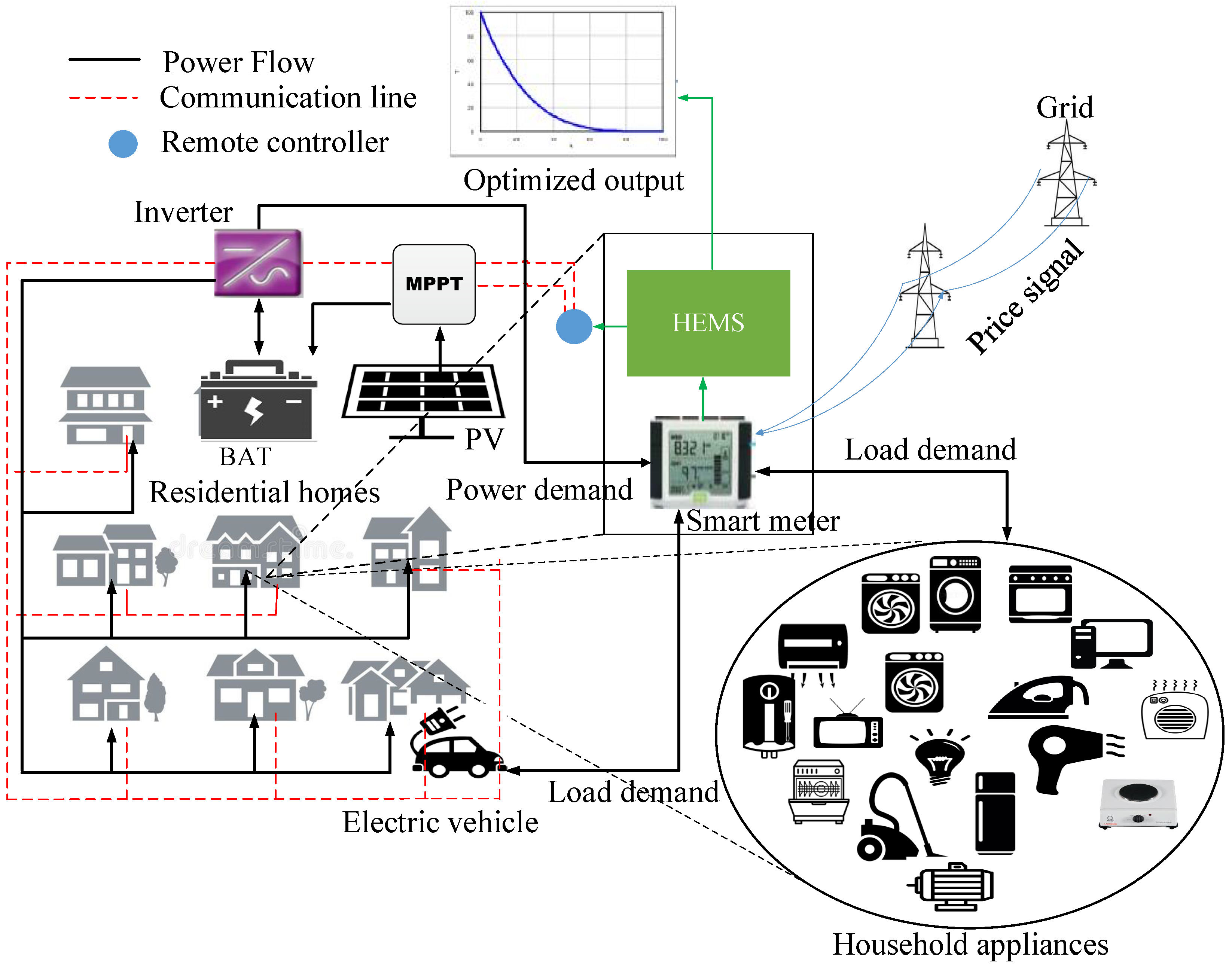
To achieve reliable management of energy and systematic operations of smart grid via DSM, a scheme of a power system that has a smart building with a number of residential households and a single utility is presented. The consumers’ electricity demands are satisfied via power grid or ESS. All consumers within the residential household have distinct electricity consumption behavior, which is related to the different load profiles. Smart meters are installed in all of the residential household for easy calculation of the electricity consumption. The smart meters ensure bidirectional communication between each residential households and utility for price sharing as well as the quantity of electricity needed to meet the load demands. We divide a day into 24 h operational time slots, for each time slot denotes one hour. We further categorize smart household appliances into shiftable and non shiftable operational mode based upon their functions.
Figure 1 shows the graphical representation of the proposed scheme that is used as the basis for developing the optimization scheme. It comprises of RES and integrated power utility that is required to meet the residential loads. The individual power grid and RES act as a node. The delivery of energy to the residential household and the ESS that are utilized during high load demands that are controlled by the optimization scheme. The residential load demand is satisfied from the power grid, where direct utilization of RES and ESS depend on the electricity price in that particular hour. However, RES and ESS are instantly used to deliver energy to the residential household. In this manner, energy demand concentrated on the power grid is drastically reduced. In addition, incorporating the RES, ESS and HEMS are beneficent at reducing the heavy load on the power grid with respect to high demand.
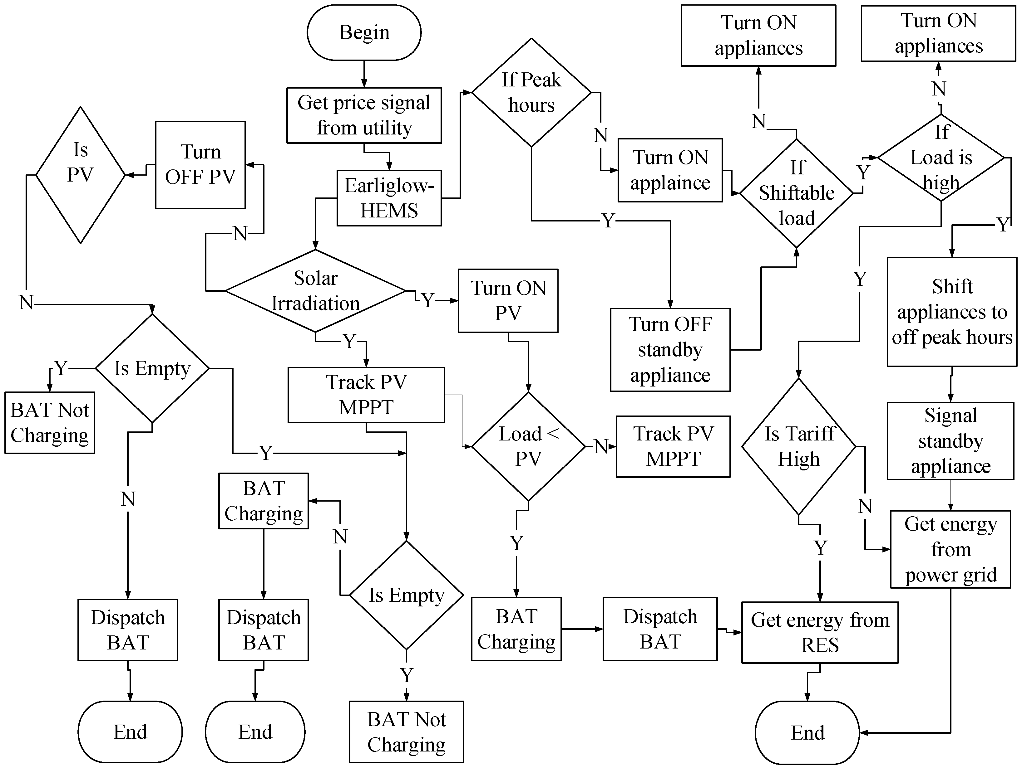
Figure 2 shows the proposed Earliglow based HEMS architecture. The electricity price signals (CPP and ToU) are obtained from the utility, which are used for electricity billing. The entire architecture is divided into two phases. Phase 1 estimates the output energy of PV that depends on several temperatures and the effect of irradiation on the PV modular. The generated energy of PV is not solely dependent on irradiation but on its surrounding temperatures. A maximum power point tracker (MPPT) is mostly used on the PV array to achieve energy output at any irradiation level. Due to cloud cover and other isolation constraints, we take a random variable of irradiation. The different irradiations and temperatures are used to calculate the maximum output energy of PV using the equation in [
33].
Once the irradiation and temperature are calculated for each hour, the PV is Turn ON. If the maximum energy output of PV is greater than the load demand of the household, thus the battery starts charging. On the other hand, if the household load is greater than the output energy of PV and the RES output is not enough to supply the household load, then the battery starts discharging. The inverter is used as the electric circuitry to convert direct current to alternative current for giving energy to the residential household. The voltage input/output, frequency and the overall energy handling depend on the system design. However, the output from the inverter is less than its input. The battery as earlier described is used for energy storage, which also enhances the energy supply to the residential household.
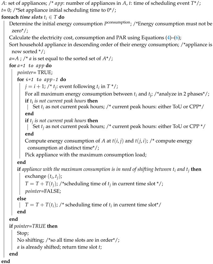
Phase 2: the actual load scheduling is performed. In this phase, the proposed Earliglow algorithm is implemented as the optimization scheme. The ideal solution derived after a series of iterative steps is converted into a binary format (0 and 1) which forms the decision variables (
Section 4.1). A 24-h scheduling plan is performed with a one hour time interval. The time periods are divided into on-peak (12–8) p.m. and off-peak (12–8) a.m. hours for the ToU signal, while we consider the on-peak hours as the critical event associated with the CPP price signal. The electricity cost, consumption and load balancing are calculated using Equations (
4)–(
6). The household appliances are sorted in descending order of their load consumption per hour. This is done in order to compare the next load from the rest of the loads. Let
denotes the event at time
i and
be the event following
at time
j. If an appliance with maximum load wants to be shifted within
and
, then swap between
and
, the appliance with maximum load is shifted to the new swapped event as presented in Algorithm 1.
| Algorithm 1: Proposed optimal scheduling technique [26] |
![Energies 11 03155 i001]() |
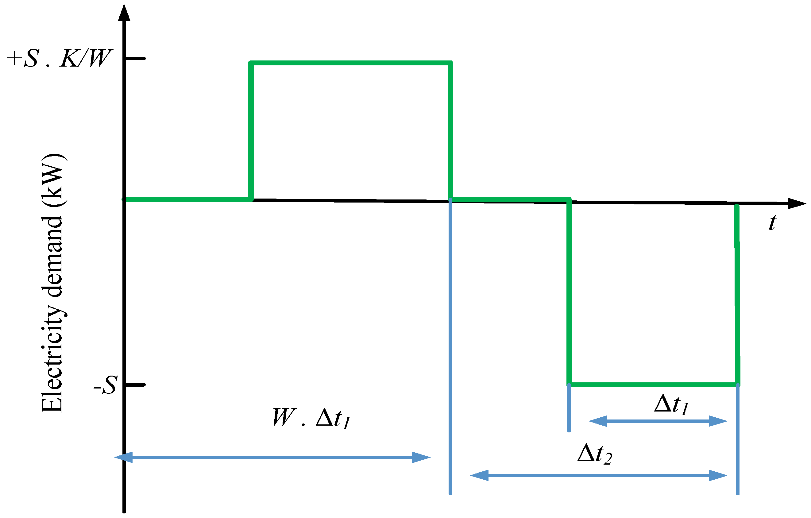
Figure 3 provides an illustration of the household load shifting activity. The change in residential load demands is characterized by the size of load reduction
, duration of load reduction
as well as duration of the load recovery, which is either greater or smaller than the load recovery
. Subsequently, the load losses between
S and load recovery
give rise to the load demand in the recovery time which may vary over load reduction. In a situation when load losses are not experienced (i.e.,
), the extra amount of power consumed in the recovery time will be equal to the energy consumed during the load reduction time. The disparity between (
) and (
) show that the recovery time does not correlate with the reduction time.
Algorithm 1 presents the optimal scheduling technique. The execution steps of the proposed optimal scheduling techniques depend on the complexity at lines (8–24) in the for-loop. The complexities of other lines (i.e., 10–22) are more than these lines. However, complexity of line 8 is influenced by line 10. All of the sub-lines 10–22 take , while line 10 can iterate maximally with a iterations, and hence its cost is . Lines 8–24 perform at the maximum iteration cost of . Then, the overall T process takes the cost of .
4.1. Jaya Algorithm
In the Jaya algorithm [
34], the objective function is presented as
and is minimized at any iteration
t. Suppose that there is a
k number of decision variables
and the number of the individual solution is presented as
l.The individual with the ideal value is presented as
in the whole individual solution. While the individual with the worse value is presented as
in the whole individual solution. If in the
jth variable we obtain the
value for the
lth individual during the
tth iteration, then we present a modified value using Equation (
11):
where
, is the value of variable
l for the ideal individual and
is value of the variable
l for the worst individual.
is the updated value of
, where
and
are two random numbers for
variable during
iteration in the range of
. The term
indicates the tendency of solution to move towards the ideal solution, whereas the term
indicates the tendency of the solution to avoid the worst solution.
is selected if it gives the ideal function value. All selected function values at each iteration are preserved and used as the input for the next iteration. Parameters used for simulation are shown in
Table 3. Algorithm 2 illustrates the proposed Jaya based HEMS.
| Algorithm 2: Proposed Jaya based HEMS [12] |
![Energies 11 03155 i002]() |
4.2. SBA
Several plant intelligence-based inspired optimization algorithms have been proposed in [
35]. The strawberry plant is generally known for its characteristic aroma, bright red color, juicy texture and its sweetness. This plant propagates via a runner in order to survive. If the plant found itself in a good spot on the ground, with plenty of soil nutrients, water and sunlight. Then, the plant produces several short runners, which reproduces a new strawberry plant and occupies the neighborhood as much as possible. On the contrary, if the strawberry plant is not on the spot of a good ground (i.e., there is no sunlight, poor nutrient and water), it will try to survive by sending fewer smaller runners to further exploit the far neighborhood, hence finding a better spot for its offspring. Since sending a longer runner is a huge investment for the plant that is in a poor spot, we therefore assumed that the quality of the spot is reflected on the growth of the plant; then, we build our optimization based on these notions: the strawberry that falls on a good spot of the ground propagates well by reproducing many short runners. Those that fall on the poor spot tends to reproduce a few long runners. The parameters of SBA are shown in
Table 3. Algorithm 3 describes the entire operations for the SBA. The
is the fitness function. Therefore, the distance between each runner and the number of the runners is computed using Equation (
12):
by default, the number of runner is proportional to its fitness and is computed using Equation (
12):
where
K is the maximum number of runner and
denotes the number of the runners generated by the solution at iteration
i after sorting.
mapped the fitness to its solution
i, where
denotes the number generated randomly for each candidate in each generation. To ensure all solutions, generate a runner for the best candidate. The
, fitness must generate at least
K maximum runner. The distance of each runner is inversely proportional to its growth and it is computed using Equation (
14):
where
j denotes the size of search space. Every
is in the range [0,1].
determines the growth of runner. The computed distance will be used for updating the
i candidate solutions, which depends on the limit of
given in Equation (
15):
The
ensures that the solution lies within the limit
, where
denote the upper and lower bound, respectively.
| Algorithm 3: SBA based HEMS |
![Energies 11 03155 i003]() |
4.3. Earliglow Algorithm
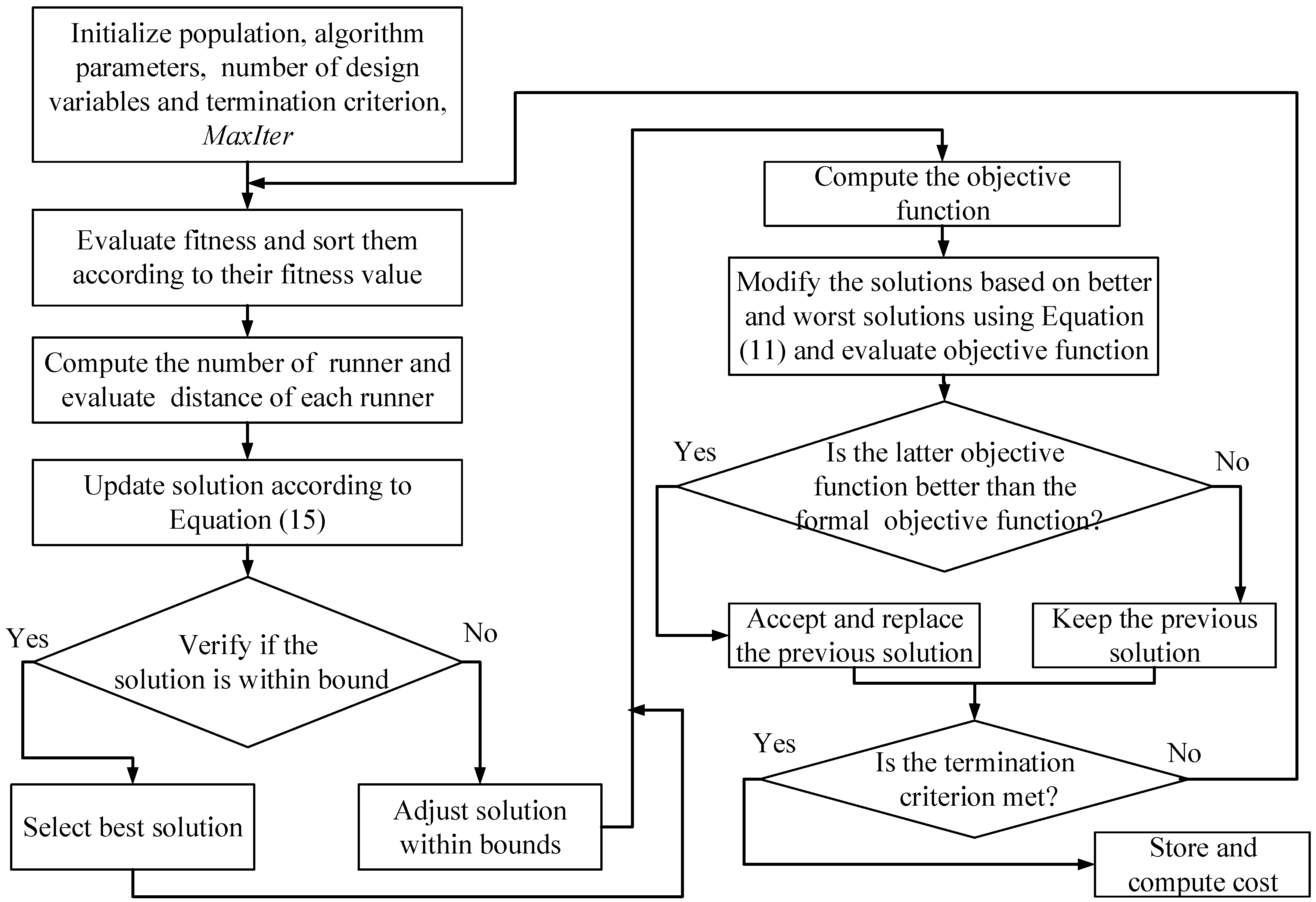
Every meta-heuristic optimization algorithms have their advantages and disadvantages. Several algorithms have a parameter tuning problem that can be resolved by trial and error. Generally, the smaller the number of tuning parameters, the more superior the algorithm is. Other limitations include an accuracy problem and high sensitivity to the initial guess while finding the global solution using low probability. In addition, achieving solutions outside the region defined by boundary values of variables. However, some algorithms may be efficient in solving one problem and yet not suitable for another. SBA has the following limitations. Firstly, SBA duplicates every number of computational individual for each iteration. Lastly, local and global searches are done simultaneously where each computational individual is subjected to large and small movement from the start to end. In addition, Jaya algorithm falls into local minimum as the number of iteration increases. To ensure the better performance of both algorithms, a new algorithm known as Earliglow which has both flavors of the existing techniques, SBA and Jaya algorithm is proposed. Based on our assumption, the named Earliglow is chosen due to its features to ripen its fruits sooner (accuracy) than other strawberry variants and is also resistant to many known strawberry diseases (fast convergence). The detailed procedures of Earliglow are illustrated in
Figure 4.
In the Earliglow algorithm, SBA algorithm is performed first on the random population using Equations (
12)–(
15) due to the problem of adjusting the individual solution within the population bounds, high memory usage, and since SBA duplicates every number of computational individual for each iteration. The Jaya algorithm is implemented to reduce the number of iterations. If the solution falls outside the given range of the defined bounds, the solution is modified on the basis of ideal and worse individual solution. For this purpose, a mutation policy is adopted as well as trimming of the population using Equation (
16). This policy updates individual solutions and ensures that the solution moves towards achieving the ideal solution while circumventing the worse solution. In addition, the number of iterations is further reduced leading to a global solution within a minimal execution time:
where mini and maxi are the minimum and maximum population bound of the
ith individual population,
x.
4.4. Enhanced Differential Evolution Algorithm (EDE)
The differential evolution (DE) algorithm was first introduced by Storn and Price in 1995 [
36], since then it has become the state-of-the-art algorithm for solving most optimization problems. This algorithm uses the concept of mutation, selection and crossover. Adjusting the common known parameters like population size, mutation, scaling factor and crossover rate. In this paper, we implement the enhanced version of DE where the performance is enhanced by adjustment of population size and scaling factor. The crossover rate is implicitly used during the crossover process. The parameters of EDE are shown in
Table 3.
5. Simulations and Discussions
In order to evaluate the performance of the proposed appliance scheduling scheme, we simulate the hourly energy use of the set of household appliances. The parameters in terms of length of operation time (LOT) and power ratings of appliance are presented in
Table 2. Simulations are performed in three cases: (I) without HEM, (II) with HEM, and (III) HEM with RES. We also discussed the hourly load behavior of household appliances and finally the feasible regions (FR) in terms of electricity cost, load and waiting time. Peak load shifting is achieved by load adjustment of appliances with feasible schedules. Shiftable appliance usage was systematically changed by turning them ON and OFF.
In this paper, consumers are charged based on the ToU and CPP pricing schemes. The ToU provides varying price structure for off-peak, mid peak and on-peak; it also provides an incentive to consumers who engage in the DR program for shifting their load to off-peak hours. In this pricing scheme, different time periods have different electricity charging rates. On the other hand, the CPP pricing scheme creates different price structure for different seasons and events of a year. The electricity cost is charged for this period with a specified rate given by the utility.
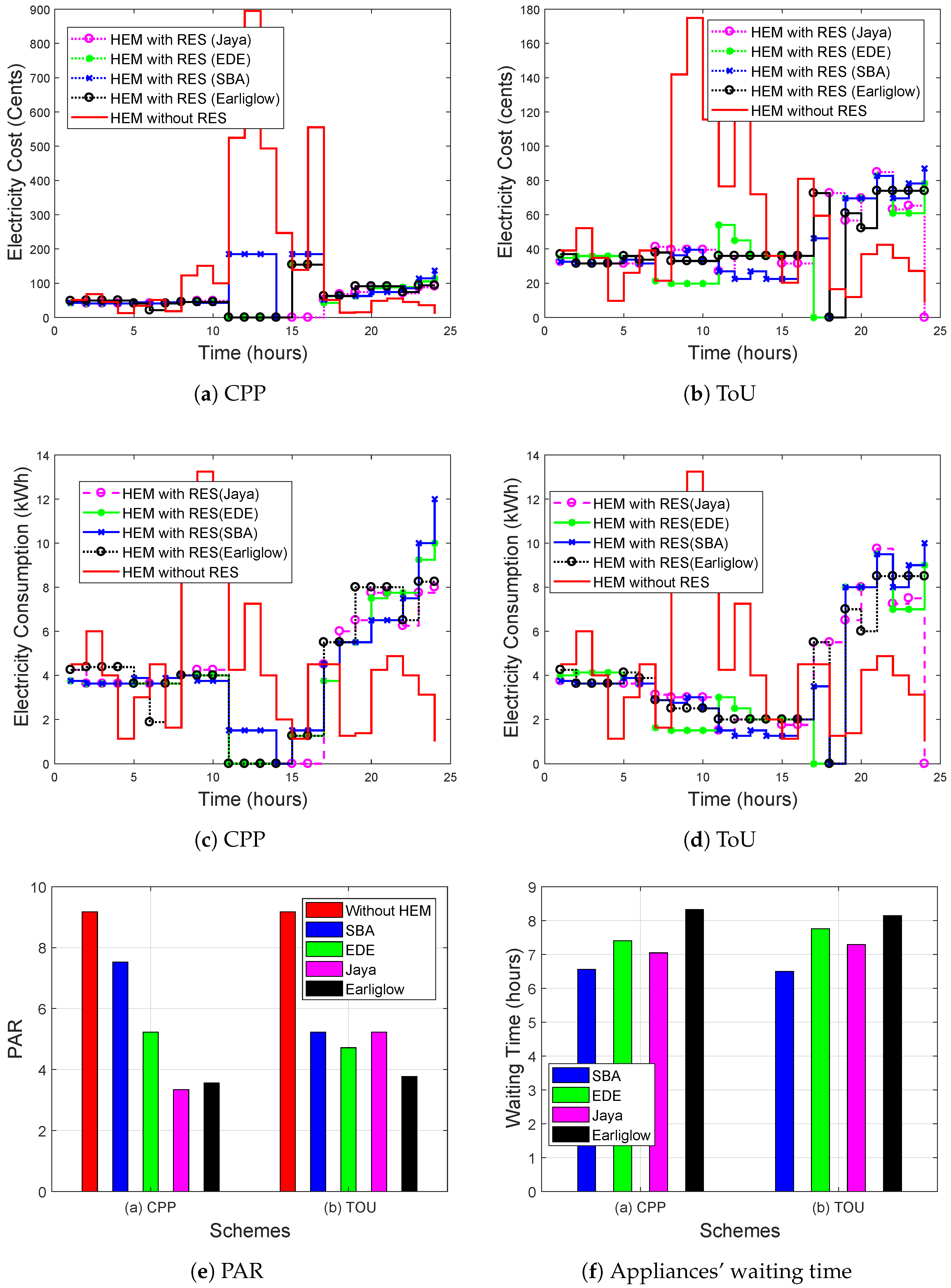
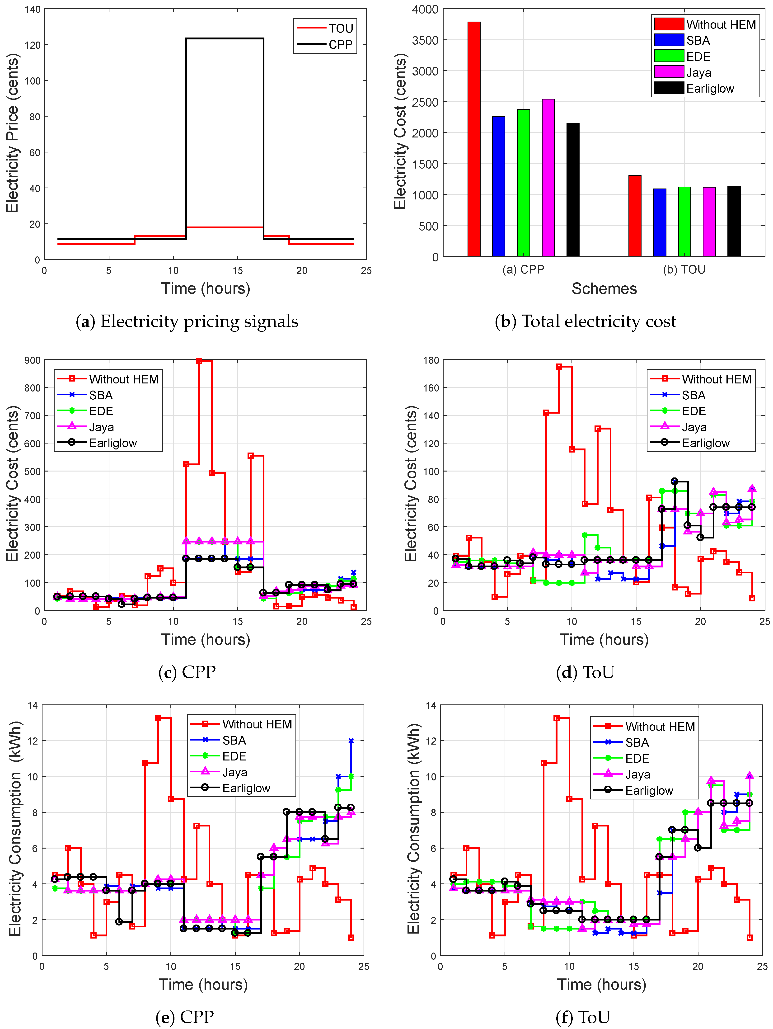
Figure 5a presents the ToU and CPP signals received from the utility and send to consumers.
5.1. Case I (without HEM)
The total electricity cost of without HEM using CPP and ToU is presented in
Figure 5b, whereas the hourly electricity cost of consumers without HEM is illustrated in
Figure 5c,d respectively.
The consumers have no HEMS architecture in their households and thus take electricity from the power grid when required.
Figure 5e,f show the different CPP and ToU pricing scheme hourly appliance consumption of energy from the main grid.
5.2. Case II (with HEM)
Four types of HEM schemes are presented to the smart consumers. The HEM scheme based on Earliglow allows few appliances to operate during on-peak hours. The achievement of Earliglow based HEM scheme is allowing optimal household appliance scheduling in the 24-h time period as presented in
Figure 5e,f, respectively. Furthermore, the electricity cost paid to utility against this consumption is presented in
Figure 5c,d, respectively. It is proven from these figures that HEMS not only shift load from on-peak to off-peak hours; however, find and shift load to the respective hours when electricity cost is minimal.
The smart consumers that implement HEM scheme based on Jaya, EDE and SBA utilize the energy optimally and stabilize the household load by moving loads from on-peak to off-peak hours by considering the different consumers’ setting and constraints. The behavior of load consumption after participating in the DR program is presented in
Figure 5e,f.
Likewise,
Figure 5c–f show the load in kWh and electricity cost in cents/h using the proposed four algorithms. The load has been scheduled from
to off-peak
for CPP, whereas the load has been scheduled from
to off-peak
for ToU. Thus, it minimizes the electricity cost and intense peak created because of load shifting where consumers depend on grid energy (
Figure 6e).
After achieving this improvement, the consumer is encouraged to engage in the effective management of energy through their household appliances scheduling. The total daily cost savings with and without HEM are presented in
Table 4. Similarly, the total daily energy savings with and without HEM are also presented in
Table 5.
In fact,
Table 4 and
Table 5 present the comparisons of the schemes used in this paper. Distinctly, the proposed scheme is efficient in the management of the household load. In addition, the penetration of RES improves it practicality for smart consumers.
5.3. Case III (HEM with RES)
In this case, the consumer employs the ToU and CPP pricing scheme and further uses the stored RES energy optimally to reduce electricity cost. The household considered in this scenario has the combination of HEM (Earliglow, Jaya, SBA and EDE) and RES generation with a storage system. The HEMS utilises the RES stored energy wherever the electricity cost of the utility is enormous and move the load from the power grid to the RES energy and therefore decreases the cost of electricity by a meaningful amount.
The achievement of all HEM schemes towards the optimal consumption of power grid depends on stored RES which is based upon the PV energy and the total area of the PV array. This means that energy can be used directly during peak hours; otherwise, it can be stored in batteries.
Huge peaks during the off-peak hours have been prevented by using the RES stored energy. During the on-peak hours, the consumers do not fully depend on the energy from the power grid and decide to use RES stored energy. In this manner, the cost of electricity and the huge peaks are drastically minimized. In addition, it will provide grid stability (
Figure 6e).
5.4. Performance Trade-Off Made by Optimization Schemes
HEMS allows consumers to optimally shift their appliances from on-peak to off-peak hours. Thus, the trade-off between cost of electricity and waiting time exists because of load shifting. The HEMS estimates the waiting time for appliances and utilizes the energy from the power grid efficiently. This enables consumer to pay a lower electricity cost and also gets the best satisfaction. Moreover, the consumer is encouraged through a reduced electric billing. Likewise, the HEMS scheduled load in order that delay is created within the operable limit. Hence, a minimum waiting time during scheduling is accepted.
Apart from RES, smart consumers are allowed to use energy optimally from the power grid and also the RES generation energy at their disposal. This class of smart consumers has HEMS that allows them to consume electricity at a low cost. The pricing schemes enable smart consumers to optimally utilize grid energy and also energy stored from RES. In conclusion, the comparisons are taken based on cost, cost savings, consumption and consumption savings.
In
Table 4, consumers without HEM pay high electricity bills for the same energy consumed by the consumers with HEM; thus, the consumer with HEM get the maximum benefit from the pricing schemes. Meanwhile, the waiting time of the consumers without HEM is little bit higher; however, they pay the maximum cost of electricity to the utility using the proposed pricing schemes. Thus, there is a trade-off between consumer’s waiting time and the cost of electricity. On the other hand, consumers with HEM pay a minimal electricity bill as compared to consumers without HEM.
The load scheduling behavior of an Earliglow based HEM scheme is smooth without creating peaks during on-peak hours. This enhances the household appliance’s operations. As shown in
Figure 5e,f, the Earliglow scheduled load in a more advanced manner and maintains the completion of the appliance’s operation. Meanwhile, the other algorithms (Jaya, EDE and SBA) demonstrate the load movement to off-peak hours efficiently.
From
Figure 5e,f, it is shown that consumers having Jaya, EDE and SBA schemes may not be able to utilize the energy stored optimally as compared to Earliglow because of high load peaks (
Figure 6e).
In conclusion, the results from the simulation confirmed the performance of Earliglow based HEM over the other HEM (Jaya, EDE and SBA) in terms of peak reduction, electricity (cost and savings), using CPP, consumption (load and savings) using the ToU scheme and computational time is presented in
Table 4 and
Table 5.
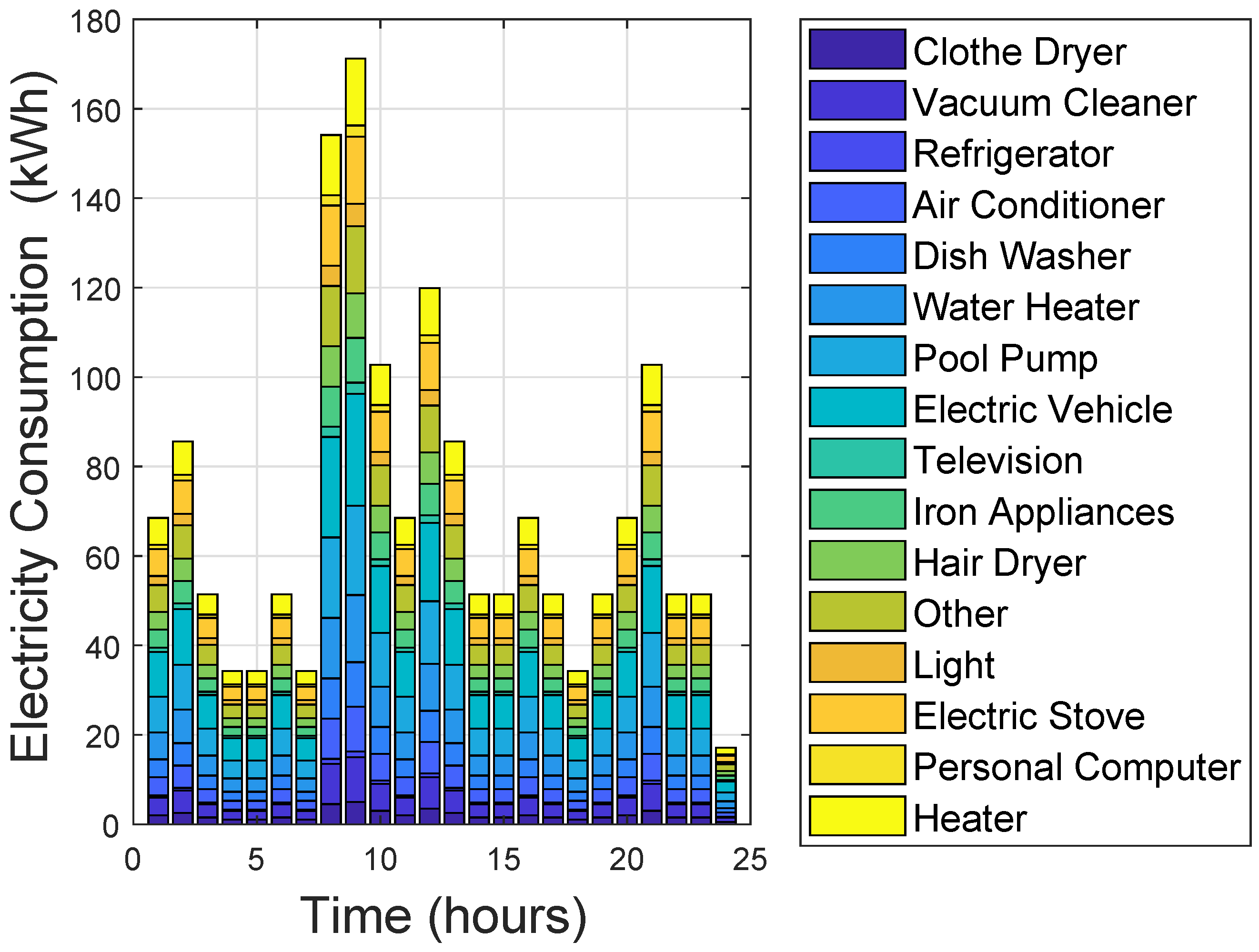
5.5. Hourly Load Behavior of Household Appliances
Figure 7 shows the consumers without HEM for hourly household appliance behavior. The figure demonstrates that the majority of the consumer household appliances are concentrated within the on-peak hours. The consumers then implement the proposed HEMS to optimally shift load from on-peak to off-peak hours as presented in
Figure 8 to illustrate the individual household appliance’s energy consumption behavior for each hour with respect to the two pricing schemes.
Using the CPP scheme: in
Figure 8a, Jaya based HEMS shift more loads to the first
and
than the other hours. Thus, the loads shifting during these hours consist of high energy consuming appliances. In
Figure 8b, most appliances are shifted to the first
and
of the day for SBA based HEMS. These are high load profile appliances like pool pump, hair dryer, iron appliance, electric stove, water heater, dishwasher and air conditioner. Finally, in
Figure 8c, most appliances are shifted to the first
and
in a day for Earliglow based HEMS than the other hours.
Using the ToU scheme: in
Figure 8d, more appliances are shifted to the
and
of the day for Jaya based HEMS than the rest hours. From these results, most of the high energy consuming loads are moved to off-peak from on-peak hours. This reduces the electricity cost and may generate peaks. While SBA based HEMS in
Figure 8e, SBA based HEMS shifts most of its appliances to the first
and
with high impact on the
. Finally,
Figure 8f shows that Earliglow based HEMS shifts most of its appliances to the first
and
of the day, especially for high load profile appliances like air conditioner, dishwasher, pool pump, iron appliances, electric stove and electric vehicle.
5.6. FR for Electricity Cost and Energy Load
A search space is the set of all possible points which satisfy the objective constraints, and it is known as the FR [
37]. In this paper, ToU price signal for all households falls within (8.70, 2317.40) cents. Similarly, ToU pricing scheme hourly energy consumption for all households in all cases falls within (1.00, 13.25) kW. In CPP, the price signal ranges from (11.40, 11,854.00) cents for all household appliances and the without HEM scheme ranges from (1.00, 13.25) kW for all the possible cases. As shown in
Figure 9, the electricity cost in the FR for each pricing scheme must be less than or equal to the maximum without HEM hourly electricity cost of 2317.40 and 11,845 cents, respectively. The following are the formulated possible cases:
The constraints obtained from the possible formulated cases in
Table 6 and
Table 7 are explained below.
The hourly cost of electricity for each load must fall within the lowest and highest electricity cost without HEM.
The hourly cost of electricity for each load must be less than the hourly electricity cost without HEM.
The entire hourly load must fall within the lowest and highest combined energy without HEM.
Based on the defined constraints, the electricity cost of scheduled loads must fall within the lower and upper limit of load without HEM hourly electricity cost. Notably, 13.25 kW is maximum hourly load without HEM which must be greater than or equal to the scheduled loads for all schemes. The FR in
Figure 9a,b, describes the relationship between electricity cost and energy load. We denote all points with
, where
is the set of points in which the without HEM load boundary lies. To calculate these points, we multiply the minimum and maximum loads with the minimum and maximum electricity price signals collected from the utility. The ToU and CPP achieve maximum electricity cost per time slot without HEM of 2317.40 cents and 11,854.00 cents, respectively. The cost for scheduled load should not be more than the electricity cost of without HEM. The FR covers all points
. The FR covers all point
. This assumes the realistic electricity cost reduction while using HEM.
5.7. FR for Cost and Waiting Time
Waiting time is measured as the amount of time the household appliances stay idle before they are turned ON.
Figure 9c,d show the FR of electricity cost versus the waiting time of each household appliance for the two pricing schemes. The shaded region indicates the points where the problem constraints are satisfied. The formulated possible case tells the average waiting time for each scheduled load per time slot and their corresponding cost. The above-formulated case is used to derive the constraints of the FR as explained below:
The hourly waiting time should not be more than the maximum average waiting cost.
The cost of hourly waiting time must be within the minimum and maximum waiting time.
The total hourly waiting time must not exceed the minimum and maximum total waiting time.
From
Figure 9c, the cost of 2210.00 cents shows the household appliance waiting time is zero, whereas, in
Figure 9d, the cost of 1080.00 cents shows zero waiting time of household appliances. From the simulation results, the maximum electricity cost for the two pricing schemes indicates the maximum delay.
6. Conclusions and Future Work
This paper proposes a model for SG that handles the emerging advancement in technology of smart households and the power grid. It is also established that integrating the RES and the proposed optimization algorithm with its solution optimally addresses the multi-objective scheduling problem. The performance of the proposed models shows that, unlike Jaya, EDE and SBA based HEMS, Earliglow based HEMS reduces the electricity cost by 43.20%, 13.83% for CPP and ToU, respectively. The proposed Earliglow based HEMS achieves a reduced PAR up to 61.23% as compared to Jaya with PAR reduction up to 63.54%, whereas SBA and EDE have PAR reduction up to 17.97% and 43.61% for the CPP scheme. Similarly, Earliglow based HEMS reduces the PAR up to 58.84% as compared to Jaya and SBA that each have PAR reduction of 43.03%, while EDE achieves PAR reduction up to 48.59% for ToU schemes. The achievements of Earliglow based HEMS over the counterparts are as follows. Firstly, Earliglow based HEMS shows that power system stability and reliable grid operation are enhanced through the efficient scheduling and utilization of the ESS. Lastly, Earliglow uses the advantages of both Jaya and SBA, which resolves the limitations of the two algorithms. Additionally, ESS is included to ensure reliable operation of the power grid as well as minimize the electricity cost. FRs illustrate the effect of household appliance scheduling on electricity cost with power consumption and consumer waiting time.
The proposed optimization method is scalable to any infrastructure capacity of the electricity system. Moreover, the proposed optimization method is efficient in achieving a global optimum solution within a small amount of execution time.
In the future, we will consider micro-grid and HEMS for minimization of the load burden on the power grid and reduction of electricity cost for the household users. We are also concerned in the coordination among the RES and ESS to utilize the renewable and sustainable energy resources. This coordination of RES in a residential area will not only enable the exchange of surplus renewable energy among the micro-grid but also minimize the load on the power grid.

 ,
, 


