Thermo-Economic Analysis of a Bottoming Kalina Cycle for Internal Combustion Engine Exhaust Heat Recovery

Abstract

The use of a Kalina cycle (KC) with a superheater to recover waste heat from an internal combustion engine (ICE) is described in this paper. The thermodynamic and economic analyses are performed for KC. The results indicate that using KC with a superheater is a feasible method to recover waste heat from ICE. The maximum thermal efficiency of KC is 46.94% at 100% ICE percentage load. The improvement of thermal efficiency is greater than 10% at all ICE loads, and the maximum improvement of thermal efficiency is 21.6% at 100% ICE load. Both the net power output and thermal efficiency of the KC subsystem increase with ICE percentage load and ammonia mass fraction. A lower turbine inlet pressure leads to a higher net power output of KC and a greater improvement of thermal efficiency when the ammonia mass fraction of the mixture is greater than 0.34. In the paper, if the same KC, which uses the largest capital investment, is used at different ICE loads, the payback period decreases with ICE load and ammonia mass fraction. In addition, both longer annual operation times and lower interest rates lead to shorter payback periods. However, it is worth noting that the payback period will be longer than the ICE’s lifetime if the ICE load is low and the annual operation time is too short.

1. Introduction

The internal combustion engine (ICE) is an important energy conversion device commonly used in automobiles, trucks, buses and ships. Though engine manufacturers have used all kinds of techniques or methods to improve thermal efficiency, approximately 60–70% of the fuel energy is taken away through coolant or exhaust. Due to the issues of energy shortage and environmental pollution, energy saving has become increasingly important. It is a feasible way to recover waste heat from ICE without increasing fuel consumption or emissions. Organic Rankine cycle (ORC) and KC are two feasible methods to recover waste heat. Because of its simplicity and adaptability for recovering waste heat at medium and low temperature, a majority of studies choose ORC for waste heat recovery. Wei et al. [1] concluded that the supercritical Rankine cycle is a suitable way to recover waste heat from a heavy-duty diesel ICE. Zhu et al. [2] analyzed the thermodynamic processes of a bottoming Rankine cycle for recovering engine waste heat and investigated the system exergy destruction with an exergy distribution map. Kostowski et al. [3] compared the ICE–ORC system with alternative throttling or expansion strategies based on a case study example. Seyedkavoosi et al. [4] proposed a novel two-parallel-step ORC for recovering waste heat from an ICE and performed an exergy analysis. Wang et al. [5] revealed that the engine working condition affects ORC dynamic response for a natural gas ICE with an ORC as the bottoming cycle. Pili et al. [6] used an ORC as the bottoming cycle to recover more than 6 kW of mechanical power from long-haul trucks waste heat, but the system would be very heavy and large. Wang et al. [7] proposed a dual-loop ORC system with R1233zd and R1234fy as the working fluid and found that this system could get better performance for similar applications than other ORC systems. Scaccabarozzi et al. [8] showed that a supercritical ORC using the optimal mixture has better thermal performance for heat recovery from heavy duty ICEs. Liu et al. [9] found that both the exergy efficiency and thermal efficiency of the MC/ORC system decreases linearly with the reduction of engine load. Wang et al. [10] illustrated that Double loop ORC (DORC) can increase the efficiency of the combined system by 12% at 60–100% engine load.

In addition to ORC, KC also shows good thermal performance for waste heat recovery due to its thermal match in heat exchangers during the heat transfer processes. Since Kalina [11] introduced KC using an ammonia-water mixture as the working fluid, many studies have been performed on KC. When KC was used as a bottoming cycle in combined cycle power plants, the thermal efficiency of KC was 30–60% higher than that of the Rankine cycle [12]; Fu et al. [13] found that compared to several other power cycles, using KC leads to an effectiveness enhancement of approximately 20% [13]. Hettiarachchi et al. [14] compared the performance of ORC and Kalina cycle system 11 (KCS11) for recovering low-temperature geothermal heat resources. They found that KCS11 has a better overall thermal performance at moderate pressures than that of ORC. Singh et al. [15] used a KC as the bottoming cycle to recover the waste heat from a coal-fired steam power plant. They found that there is an optimal ammonia mass fraction that produces the maximum cycle efficiency for a given turbine inlet pressure. Li et al. [16] found KC has better thermo-economic performance than that of the CO₂ transcritical power cycle by using low-temperature geothermal water as their heat resources. Yari et al. [17] compared the thermodynamic and economic performance of KCS11, ORC and the trilateral power cycle (TLC) and found that the net power from TLC is higher than that of KCS11 and ORC. Wang et al. [18] analyzed a composition-adjustable KC and found that the composition adjustment can improve system performance significantly. Fallah et al. [19] found that KC has high potential for efficiency improvement. Nemati et al. [20] concluded that ORC has significant advantages over KC for waste heat recovery from CGAM cogeneration system. Gharde et al. [21] believed that KC would be suitable for waste heat recovery for its high thermal efficiency and designed a KC subsystem to recover waste heat from a 1196 cc multi-cylinder petrol engine. Yue et al. [22] found that the transcritical ORC has higher overall thermal efficiency than that of KC for waste heat recovery under various different ICE working conditions.

In brief, a review of the published literatures indicates that both ORC and KC have promising thermal performance for recovering low- and moderate-temperature waste heat. However, few investigations focused on the thermodynamic and economic analyses of a bottoming KC for waste heat recovery from ICE. The ICE-Kalina system, composed of a topping ICE and a bottoming KC with a superheater, is proposed in this paper to recover waste heat from ICE. The thermodynamic and economic analyses are conducted for bottoming KC. The effects of several important parameters on thermal and economic performance, such as ICE percentage load and ammonia mass fraction, are investigated.

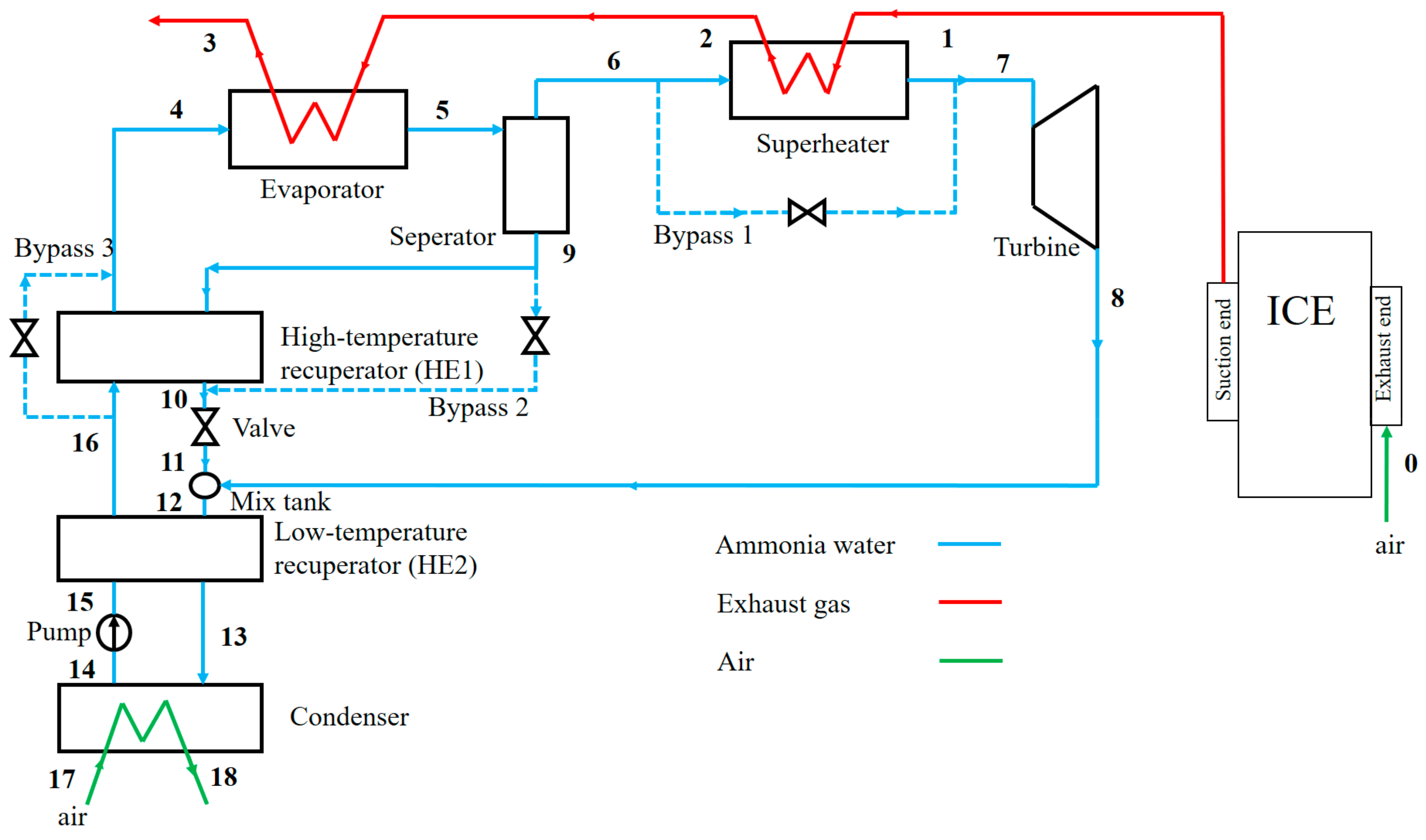
2. System Description and Assumptions

A schematic diagram of bottoming KC with a superheater for ICE waste heat recovery is shown in Figure 1. The waste heat of ICE is the heat source of bottoming KC. The working fluid of KC is an ammonia-water mixture. The main components of KC are evaporator, separator, superheater, low-temperature recuperator and high-temperature recuperator, turbine, condenser, and pump.

The ammonia-water mixture is heated in the evaporator (state 5), and then is separated into a saturated ammonia-water vapor (state 6) and an ammonia-water liquid (state 9) in the separator. After the separator, the separated ammonia-water vapor goes into the superheater to increase its temperature. Next, the vapor passes through the turbine (state 8) to generate power. Saturated ammonia-water liquid (state 9), after absorbing some heat in the high-temperature recuperator (state 10), is throttled down to a low pressure (state 11) and mixed with the ammonia-water vapor leaving the turbine in the mix tank (state 12). After that step, the ammonia-water mixture enters the low-temperature recuperator to preheat the ammonia-water solution at its cold side. Next, the ammonia-water mixture (state 13) releases heat in the condenser and increases pressure through the pump (state 15). Then the ammonia-water mixture flows to the evaporator via the low- and high-temperature recuperators, sequentially.

If T₁ is low, the ammonia-water vapor (state 6) will go to the turbine through bypass 1 instead of flowing through the superheater. When T₉ is lower than T₄, the working fluids at state 9 and state 16 will not flow through the high-temperature recuperator and will go to the valve and the evaporator through bypasses 2 and 3, respectively.

The following assumptions are used in this work:

• The KC subsystem does not influence the operation condition of ICE.
• The KC system operates in a steady-state.
• Changes in kinetic and potential energies are negligible.
• The pressure loss due to frictional effects is negligible.
• The ammonia-water mixture leaving the condenser (state 14) is a saturated liquid.
• The minimum pinch-point temperature difference of all heat exchangers is 10K.

3. System Modeling

3.1. Thermodynamic Modeling

For thermodynamic analysis, the principles of mass and energy conservations are applied to each component. The energy relations for the equipment of the ICE-Kalina system are listed in

Table 1. Energy relations for equipment of the ICE-Kalina system.

Subsystem	Equipment	Energy Equations
The topping ICE system		$Q_0=P_{ICE}+Q_{loss}+Q_1+Q_2$
		$Q_3=m_1{c}_p\left(T_1-T_3\right)=Q_{eva}+Q_{\sup }$
The bottoming Kalina cycle	Evaporator	$Q_{eva}=m_4\left(h_5-h_4\right)=m_1\left(h_2-h_3\right)$
	Superheater	$Q_{sup}=m_6\left(h_7-h_6\right)=m_1\left(h_1-h_2\right)$
	Separator	$m_9{h}_9+m_6{h}_6=m_4{h}_5$
	HE1	$m_9\left(h_9-h_{10}\right)=m_4\left(h_4-h_{16}\right)$
	HE2	$m_9\left(h_{12}-h_{13}\right)=m_4\left(h_{16}-h_{15}\right)$
	Condenser	$Q_{con}=m_9{h}_{13}-m_4{h}_{14}$
	Turbine	$W_T=m_6\left(h_7-h_{8,s}\right){\eta }_{s,T}$
	Pump	$W_p=m_4\left(h_{15,s}-h_{14}\right)/{\eta }_{s,p}$
	Throttle valve	$h_{10}=h_{11}$
	Mix tank	$m_9{h}_{11}+m_6{h}_8=m_4{h}_{12}$

.

Q₀ is the overall fuel heating value during combustion. Q₁ is the cooling heat taken away by the coolant and lubricant. Q₂ is the waste heat of the exhaust exiting the ICE. Q_loss is the heat loss of the engine thermodynamic cycle. P_ICE is the net power output of the ICE system. Q₃ is the waste heat recovered by bottoming KC [22]. η_s,T and η_s,P represent the isentropic efficiencies of the turbine and the pump, respectively; both are 0.85 in this paper.

The net power output of the ICE-Kalina system, including the net power outputs of ICE and KC, can be defined as follows:

$$W_{net}=P_{ICE}+W_{net,Kalina}$$

(1)

The overall thermal efficiency of the ICE-Kalina system is defined as follows:

$${\eta }_t=\frac{P_{ICE}+W_{net,Kalina}}{Q_0}$$

(2)

Thermal efficiency of the topping ICE subsystem is calculated by:

$${\eta }_{t\_ICE}=\frac{P_{ICE}}{Q_0}$$

(3)

Improvement of the thermal efficiency is calculated by:

$$\Delta {\eta }_t=\frac{{\eta }_t-{\eta }_{t\_ICE}}{{\eta }_{t\_ICE}}$$

(4)

The exergetic efficiency of the evaporator in KC is defined by:

$${\eta }_{ex\_evp}=\frac{E_{x5}-E_{x4}}{E_{x2}-E_{x3}}$$

(5)

The exergetic efficiency of the superheater in KC is defined by:

$${\eta }_{ex\_sup}=\frac{E_{x7}-E_{x6}}{E_{x1}-E_{x2}}$$

(6)

The exergetic efficiency of KC is defined by:

$${\eta }_{ex\_Kalina}=\frac{W_{net\_Kalina}}{E_{x1}-E_{x3}}$$

(7)

Verification of Ammonia-Water Thermodynamic Properties

A MATLAB (R2014a, MathWorks, Natick, MA, USA) code has been developed to conduct the numerical simulations for the ICE-Kalina system. The thermodynamic properties of the ICE exhaust gas are evaluated by REFPROP (Version 9.0, National Institute of Standards and Technology (NIST), CO, USA) The thermodynamic properties of the KC states are evaluated by the method proposed by Xu and Goswami [23].

To verify the thermodynamic models for KC in the paper, data available in the published literature are used. The numerical models have been validated using data from Ref. [22] under the same operating conditions. Comparisons between the simulation results and those from Ref. [22] are presented in

Table 2. Validation of the numerical model with the published data.

Parameter	Pressure/bar		Temperature/K		Mass Rate/m3/kg		Ammonia Mass Fraction
No.	Simulation	Ref. [22]	Simulation	Ref. [22]	Simulation	Ref. [22]	Simulation	Ref. [22]
4	53	53	437	433	2.07	2.06	0.37	0.37
5	53	53	494	494	2.07	2.06	0.37	0.37
6	53	53	494	494	0.71	0.668	0.584	0.616
8	3.97	3.97	382	381	0.71	0.668	0.584	0.616
9	53	53	494	494	1.36	1.39	0.247	0.252
10	53	53	388	380	1.36	1.39	0.247	0.252
11	3.97	3.97	352	345	1.36	1.39	0.247	0.252
13	3.97	3.97	337	334	2.07	2.06	0.37	0.37
14	3.97	3.97	301	301	2.07	2.06	0.37	0.37
15	53	53	302	302	2.07	2.06	0.37	0.37

. The data in Table 2 shows a little difference between the simulation results of this paper and those in Ref. [22]. This is because the thermodynamic properties in Ref. [22] are simulated via the simulation platform of Aspen Plus, and the thermodynamic properties of ammonia-water mixture in this paper are evaluated by the method proposed by Ref. [23]. The thermal efficiency of KC in Ref. [22] is 18.8%, and the efficiency of KC without the superheater in this paper is 19.4%. Therefore, the data in Table 2 still indicate a good agreement between the simulation results of this paper and those in the published literature.

3.2. Economic Modeling

To evaluate the thermo-economic performance of the Kalina subsystem, the payback period for KC is analyzed in this paper.

It is necessary to get the total capital cost of KC to calculate the payback period. According to Ref. [24], the heat exchangers, pump and turbine contribute largely to the total cost. This finding is reasonable because 80–90% of the capital cost of the system is attributed to heat exchangers [25]. We assume that all of the heat exchangers in the KC system are shell-and-tube heat exchangers [26,27].

The total heat transfer rate per unit time, can be calculated by [28]:

$$Q=UA\Delta T_m=UA\left[\frac{\left(\Delta T_{\max }-\Delta T_{\min }\right)}{\ln \left(\Delta T_{\max }/\Delta T_{\min }\right)}\right]$$

(8)

It is tedious to determine the overall heat transfer coefficient U, and the data needed in this instance are not available at the preliminary stages of the design. Therefore, for preliminary calculations, as a first approximation, the values of the overall heat transfer coefficient are given in

Table 3. Overall heat transfer coefficients for heat exchangers [29].

Component	Overall Heat Transfer Coefficient (W/m2K)
Evaporator	1100
Conderser	500
Superheater	300
Recuperator	700

[29].

The equipment module costing method is used to evaluate the equipment costs. Considering the impact of inflation, the Chemical Engineering Plant Cost Index (CEPCI) is used to convert the total equipment cost of the system at the base time into that of the year of 2017 [30], which is expressed as:

$$C_{2017}=C_b\left(\frac{I_{2017}}{I_b}\right)$$

(9)

where C_b is the cost at the base time, and I₂₀₁₇ and I_b are the cost indices assigned 567.5 [31] and 397 [30], respectively.

If the equipments are made of carbon-steel and operate at ambient pressures, the purchased cost of the equipment can be calculated by [30]:

$$\lg C_{eq}^0=K_1+K_2\lg Z+K_3{(\lg Z)}^2$$

(10)

where $C_{eq}^0$ is the purchased cost of the equipment at ambient pressures using carbon steel construction and Z is the capacity of the equipment. For the heat exchanger, Z refers to the area of heat exchange A. For the pump, Z refers to the power consumption of the pump, W_p. For the turbine, Z represents the power output, W_T. For the separator, Z represents the volume of the separator, V_sep. The coefficients of K₁, K₂ and K₃, are listed in

Table 4. Constants for equipment costs calculation [30].

Constant	Value	Constant	Value	Constant	Value
K1,he	4.3247	K2,pump	0.0536	C2,he	0.11272
K2,he	−0.303	K3,pump	0.1538	C3,he	0.08183
K3,he	0.1634	B1,he	1.63	C1,pump	−0.3935
K1,turb	2.7051	B2,he	1.66	C2,pump	0.3957
K2,turb	1.4398	B1,sup	2.25	C3,pump	−0.00226
K1,sup	3.4974	B2,sup	1.82	FM,he	1
K2,sup	0.4485	B1,pump	1.89	FBM,turb	3.5
K3,sup	3.4974	B2,pump	1.35	FM,sep	1
K1,pump	3.3892	C1,he	0.03881	FM,pump	2.2

.

Assuming each heat exchanger of the system is a carbon-steel shell-and-tube heat exchanger, the cost is given by [30]:

$$C_{he}=\frac{567.5}{397}{C}_{he}^0\left(B_{1,he}+B_{2,he}{F}_{M,he}{F}_{p,he}\right)$$

(11)

where B_1,he and B_2,he are constants based on the type of heat exchanger, F_M,he is the material factor and F_P,he is the pressure factor, which is calculated as [30]:

$$lg{F}_{p,he}=C_{1,he}+C_{2,he}lg{p}_{he}+C_{3,he}{\left(lg{p}_{he}\right)}^2$$

(12)

where C_1,he, C_2,he and C_3,he are constants in terms of the type and pressure range of the heat exchanger.

The turbines in this work are made of carbon steel with axial types; their costs are calculated as [30]:

$$C_{turb}=\frac{567.5}{397}{C}_{{}_{turb}}^0{F}_{BM,turb}$$

(13)

where F_BM,turb refers to the bare module factor according to the type and material of construction of the turbine.

For the separator, carbon steel and vertical type are chosen for construction. The cost is expressed as [30]:

$$C_{sep}=\frac{567.5}{397}{C}_{sep}^0\left(B_{1,sep}+B_{2,sep}{F}_{M,sep}{F}_{p,sep}\right)$$

(14)

where B_1,sep and B_2,sep are constants according to the type of separator, F_M,sep is the material factor and F_p,sep is the pressure factor, which is calculated by [30]:

$$F_{p,sep}=\max \left\{\frac{\frac{\left(p_{sep}+1\right)\cdot D_{sep}}{2\cdot \left[850-0.6\cdot \left(p_{sep}+1\right)\right]}+0.00315}{0.0063},1\right\}$$

(15)

The pumps are centrifugal and made from stainless steel; their costs are given by [30]:

$$C_{pump}=\frac{567.5}{397}{C}_{pump}^0\left(B_{1,pump}+B_{2,pump}{F}_{M,pump}{F}_{p,pump}\right)$$

(16)

where B_1,pump and B_2,pump are constants in terms of the type of the pump, F_M,pump is the material factor and F_P,pump is the pressure factor, which is given by [30]:

$$lg{F}_{p,pump}=C_{1,pump}+C_{2,pump}lg{p}_{pump}+C_{3,pump}{\left(lg{p}_{pump}\right)}^2$$

(17)

where C_1,pump, C_2,pump and C_3,pump are constants according to the type and pressure range of the pump.

The constants mentioned above are all listed in Table 4.

The capital recovery factor (CRF) is defined as follows [30]:

$$CRF=\frac{i{\left(1+i\right)}^{T_s}}{{\left(1+i\right)}^{T_s}-1}$$

(18)

where i is the interest rate (4.3%) [32,33]. The economic lifetime of the ICE-Kalina system (T_s) is 15 years [32]. The payback period is given by:

$$\left(W_{net\_Kalina}\cdot O{P}_s\cdot C_{pri}-CO{M}_s\right)\cdot \left(\frac{{\left(1+i\right)}^{\tau }-1}{i\cdot {\left(1+i\right)}^{\tau }}\right)=C_{2017}$$

(19)

Next, the payback period of the system is evaluated by Equation (19) [33]:

$$\tau \approx \frac{C_{2017}}{\left(W_{net\_Kalina}\cdot O{P}_s\cdot C_{pri}-CO{M}_s\right)\cdot \left(1-i\right)}$$

(20)

where C_pri is the price of electricity (the price of electricity in China in 2017 is approximately 0.63 yuan/kWh, which is 0.1 $/kWh based on the ratio of RMB to USD) [34]. OP_s is the annual operation time, which changes from 3700 to 8500 h in the paper. COM_s is the system operational and maintenance costs (1.65% of C₂₀₁₇) [35].

The Kalina subsystem used for ICE waste heat recovery can reduce the fossil fuel consumption and CO₂ emission. If KC is used instead of a petroleum-fired power plant, the annual saved petroleum M_pe (kL/year) and reduced CO₂ emission M_em (kg/year) can be estimated as [36]:

$$M_{pe}=O{P}_s\cdot a_{pe}\cdot W_{net\_Kalina}$$

(21)

$$M_{em}=O{P}_s\cdot a_{em}\cdot W_{net\_Kalina}$$

(22)

where a_pe is the amount of petroleum consumed to produce 1 kWh of electrical energy and a_em is the amount of CO₂ emissions if 1 kWh of electrical energy is produced by a petroleum-fired power plant. The values are assumed as follows: a_pe = 0.266 L/(kWh) and a_em = 0.894 kg/(kWh) [36].

4. Results and Discussion

4.1. Thermal Performance Analysis for KCs

Table 5. Waste exhaust parameters at different ICE loads [22] (p₁ = 101 kPa).

ICE Load Percentage	Fuel Total Heating Value Q0 (kW)	Power Output PICE (kW)	Thermal Efficiency of ICE ηt_ICE (%)	Exhaust Gases Temperature T1 (K)
100	5590	2000	35.78	712
90	5050	1800	35.64	683
80	4560	1600	35.09	660
75	4330	1500	34.64	649
70	4110	1400	34.06	638
60	3640	1200	32.97	618
50	3120	1000	32.05	596
40	2580	800	31.01	569
30	2050	600	29.27	535
25	1810	500	27.62	514
20	1560	400	25.64	491
10	1060	200	18.87	419

gives the waste exhaust operation parameters at different ICE percentage loads for 3561CDITA ICE [22]. The thermodynamic performance of the proposed system at full load is calculated.

Table 6. Primary thermodynamic performance indices of bottoming cycle.

Items	Value	Value in Ref. [22]	Items	Value	Value in Ref. [22]
ICE load percentage (%)	100%	100%	Q3 (kW)	920	1151
fuel total heating value Q0 (kW)	5590	5590	Q4 (kW)	448	935
power output PICE (kW)	2000	2000	WT_Kalina (kW)	436.6	217
exhaust gases volume flow rate (m3/s)	7.2	7.2	Wnet_Kalina (kW)	432
exhaust gases temperature T1 (K)	712	712	ηt_kalina (%)	46.94	18.8
turbine inlet temperature T7 (K)	692	494	ηt_ICE (%)	35.78	35.78
turbine inlet pressure p7 (bar)	30	53	Δηt (%)	21.6	15.1
ammonia mass fraction x4	0.56	0.37	payback period (year)	2.94
m4 (kg/s)	0.985		Mem (tons/year)	1691
m6 (kg/s)	0.952		Mpe (kL/year)	503.2

gives the parameters of some states in the Kalina subsystem at 100% ICE load.

The thermodynamic performance of the ICE-Kalina system is calculated and compared with Ref. [22], as illustrated in Table 6. The results show that the heat recovered from the ICE, the turbine work and the net power output of the ICE-Kalina system are 920 kW, 436.6 kW and 432 kW, respectively. The overall thermal efficiency of the ICE-Kalina system is 43.5%. Compared with the ICE system, the improvement of the thermal efficiency is 21.6%. The thermal efficiency of the proposed subsystem is much higher than the subsystem in Ref. [22]. This finding is observed because the KC with a superheater has a better thermal match in the heat transfer exchangers than the KC without a superheater in Ref. [22], especially at high exhaust inlet temperatures. This means that when the ICE load is high, the proposed Kalina subsystem with a superheater is more efficient than the Kalina subsystem in Ref. [22].

The Kalina subsystem could effectively reduce CO₂ emissions and petroleum consumption. Under the working conditions shown in Table 6, 503.2 kL of petroleum was saved and 1691 tons CO₂ was reduced per year. These data indicate that using the Kalina subsystem is an effective way to reduce the petroleum consumption and reduce the emission of CO₂.

4.2. Thermal Performance

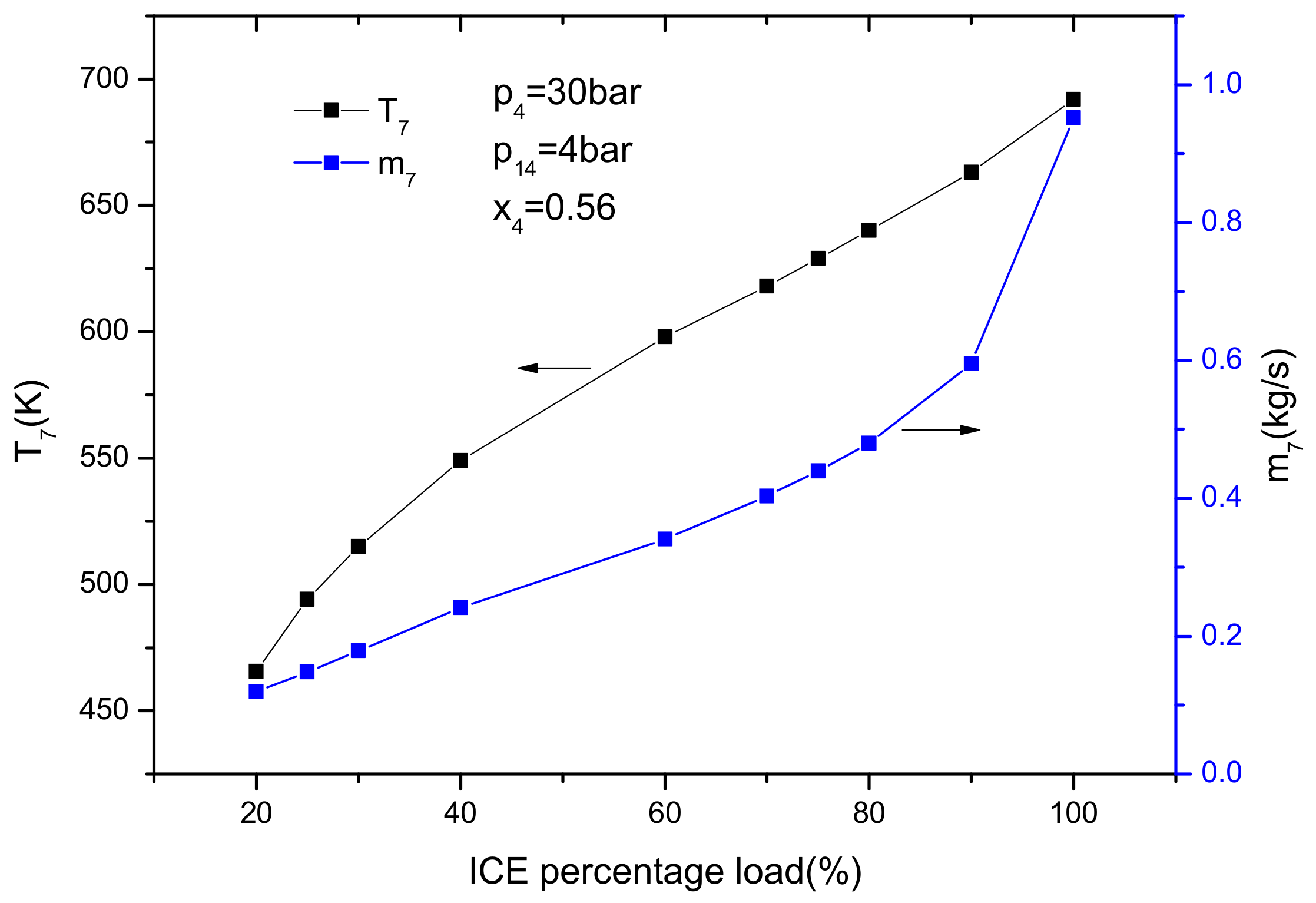
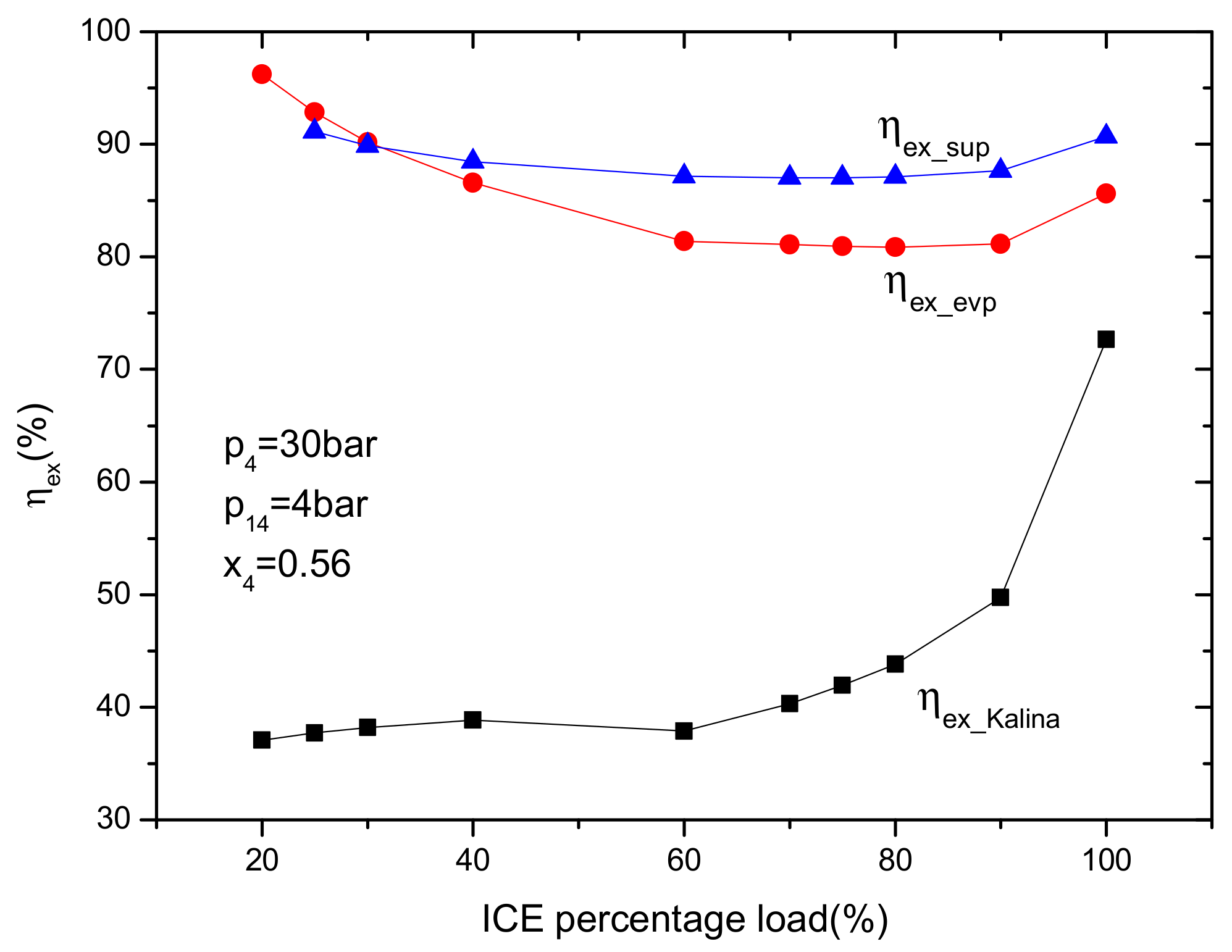
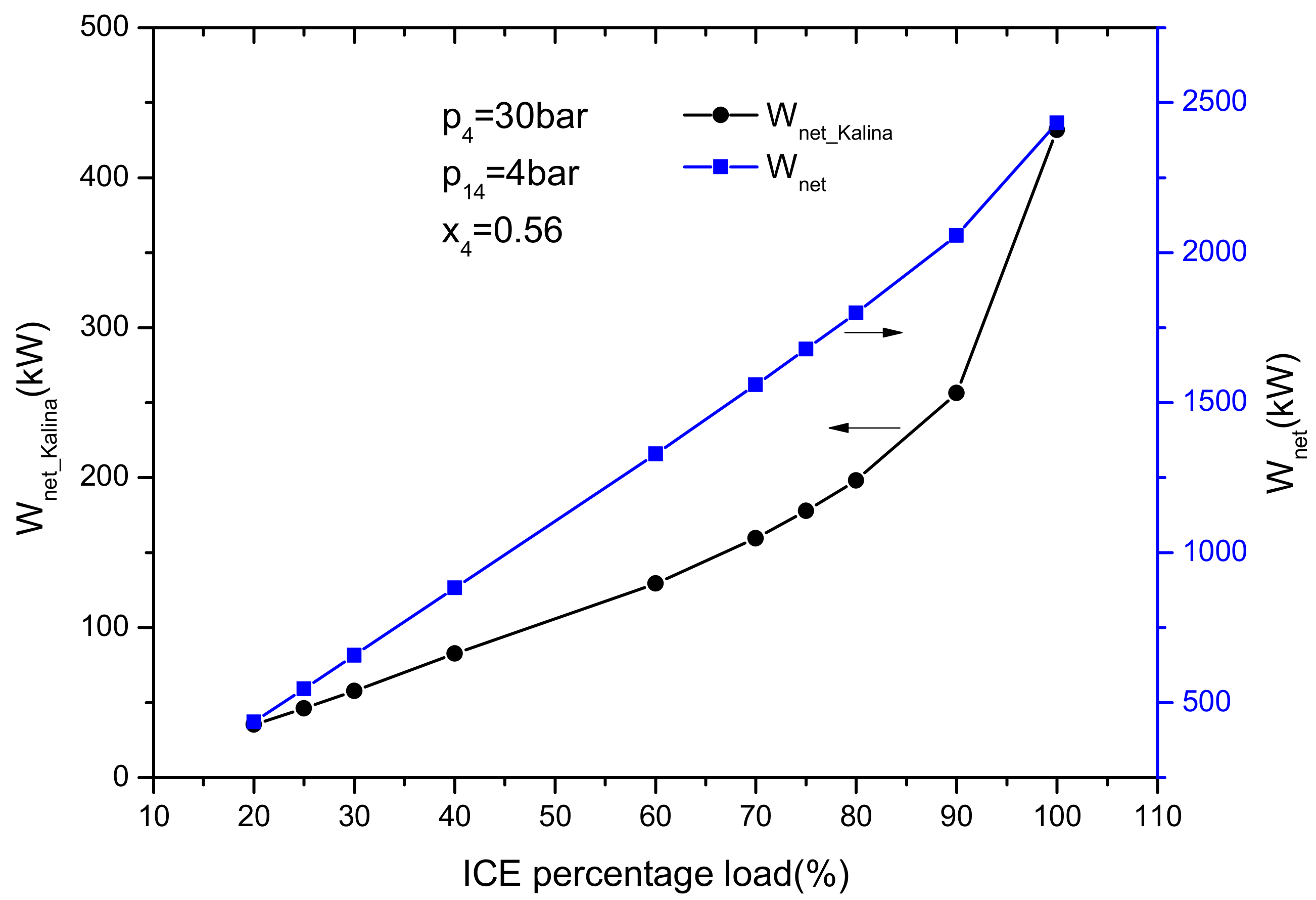
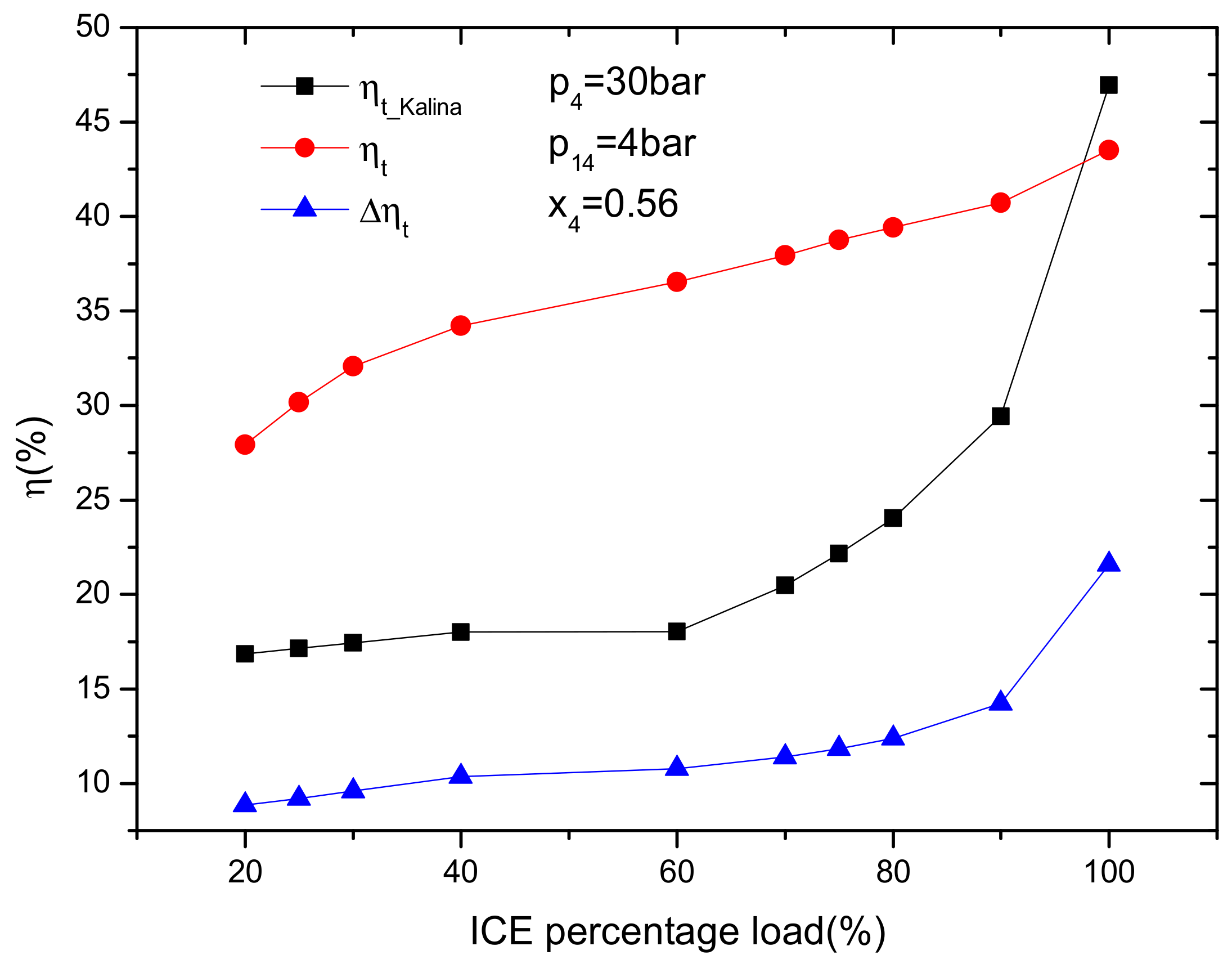
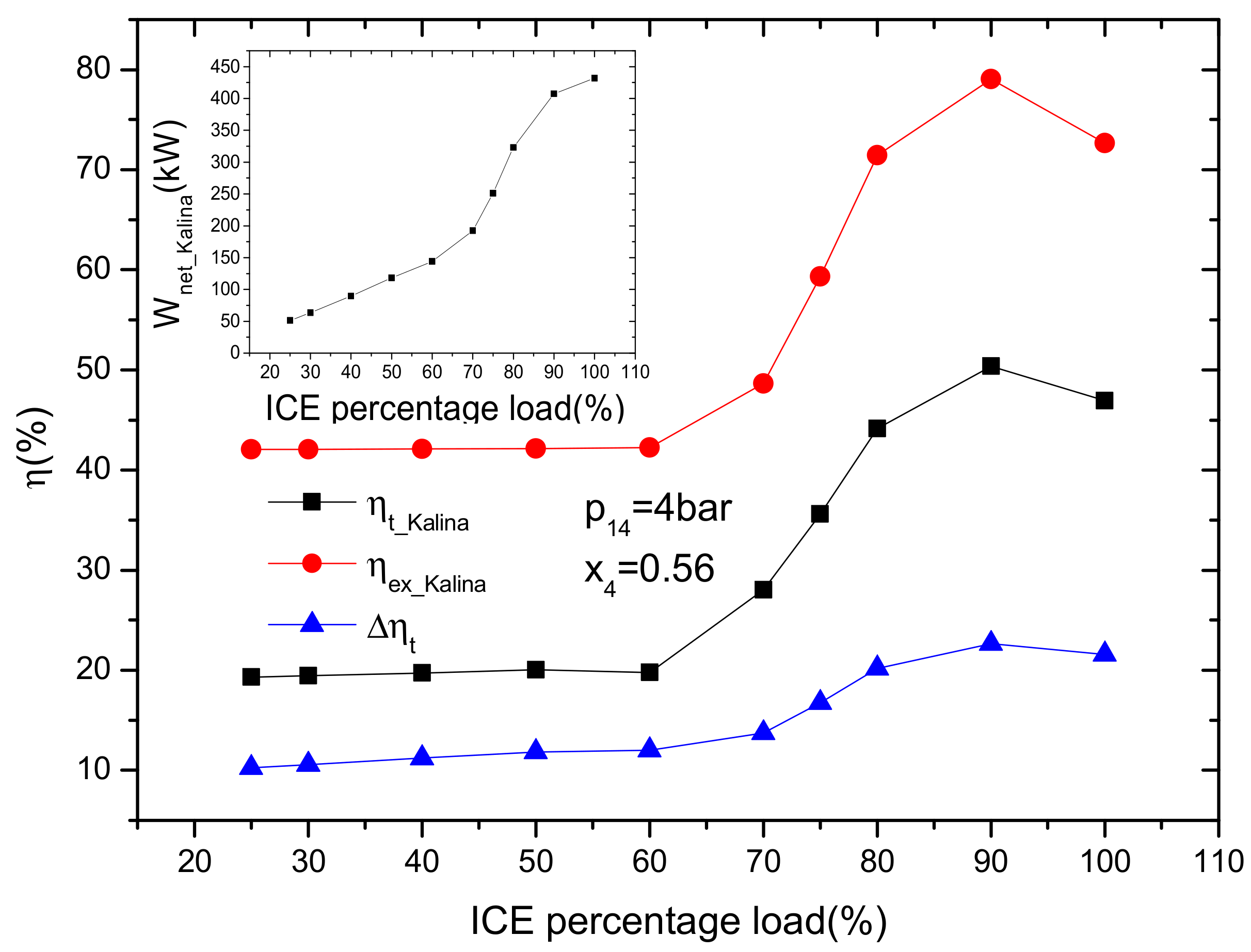
4.2.1. Effect of the ICE Load

The ICE load is an extremely important operation parameter for the Kalina subsystem using the exhaust as its heat resource because it influences the temperature (T₁) and mass flow rate (m₁) of the exhaust gas. The temperature and mass flow rate of the exhaust gas increase with the ICE load. As shown in Figure 2, higher ICE percentage loads affect the turbine inlet temperature (T₇) and the mass flow rate of the ammonia-water vapor (m₇).

Figure 3 shows the effect of ICE percentage load on the exergy efficiency of the evaporator (η_{ex_evp}), superheater (η_{ex_sup}), and KC (η_{ex_Kalina}). Both the exergy efficiencies of the evaporator and the superheater decrease first and then increase with ICE load and are greater than 80% at all ICE loads due to the good thermal match of the evaporator and the superheater. The exergy efficiency of the evaporator and the superheater reach their maximum values at 20% and 25% ICE load, respectively. The exergy efficiency of KC increases with ICE load. The increase of the exergy efficiency of KC becomes greater when the ICE load is greater than 60%. This is because the growth of W_{net_Kalina} is larger from 60% to 100% load, while the growth of (E_x1−E_x3) is smaller in this load range. The exergy efficiency of KC has its maximum value at 100% ICE load.

If the turbine outlet pressure is fixed, the enthalpy drop in the turbine increases with increasing turbine inlet temperature. Therefore, the net power output of both KC (W_{net_Kalina}) and the ICE-Kalina system (W_net) increases as the ICE percentage load increases (Figure 4). As shown in Figure 5, the thermal efficiency of KC (η_{t_Kalina}), the overall thermal efficiency of ICE-Kalina system (η_t) and the improvement of thermal efficiency of ICE (Δη_t) increase with ICE percentage load. When ICE percentage load is at 100% with a turbine inlet pressure of 30 bar and an ammonia mass fraction of 0.56, the improvement of thermal efficiency of ICE is 21.6%.

Figure 6 shows the maximum value of the net power output of KC, the thermal efficiency of KC, the overall thermal efficiency of ICE-Kalina system, the improvement of thermal efficiency of ICE and the exergy efficiency of KC at different ICE loads. The optimal net power output of KC increases with the ICE load. The maximum thermal efficiency of KC increases first, has a maximum value at 90% ICE load and then later decreases. This effect is due to the greater increase of waste heat recovered by bottoming KC (Q₃) than that of the net power output of KC at 100% ICE load. Moreover, all values of the maximum improvement of thermal efficiency are greater than 10% at all ICE loads. The minimum improvement of thermal efficiency is 10.3% at 25% ICE load. This means that using KC with superheat is a feasible method to recover ICE waste heat. The maximum exergy efficiency of KC has a similar trend as maximum thermal efficiency and achieves its maximum value at 90% ICE load. According to the comparison, it is concluded that the maximum net power output and the thermal efficiency of KC in this paper are greater than those reported in Ref. [22] at all ICE loads, and the values of maximum exergy efficiency are greater than those in Ref. [22] when the ICE load is greater than 40%.

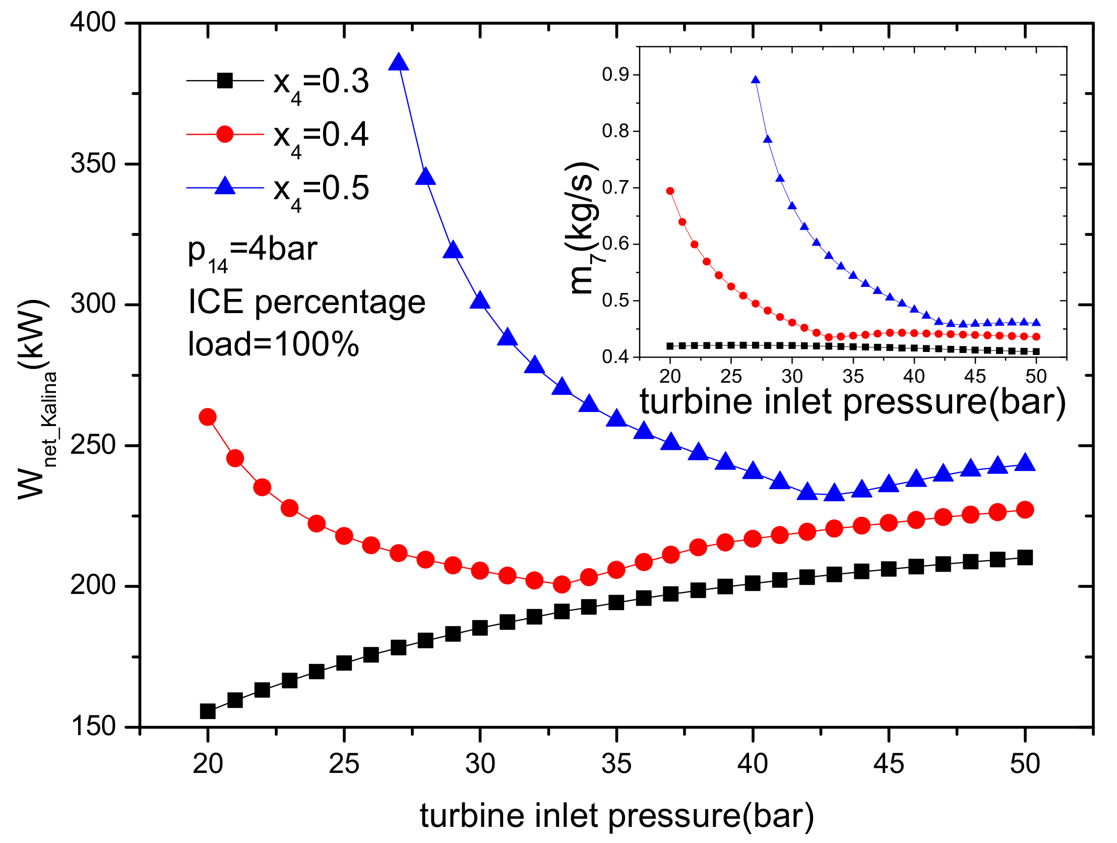
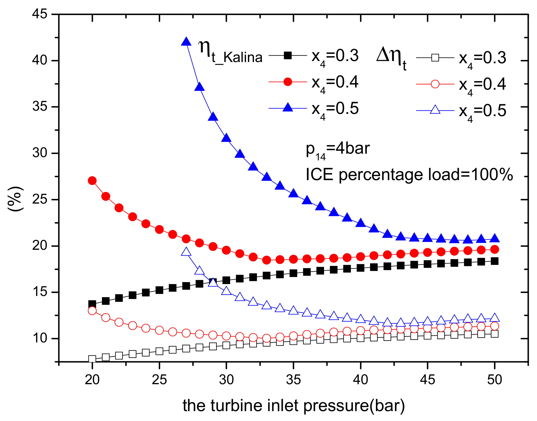
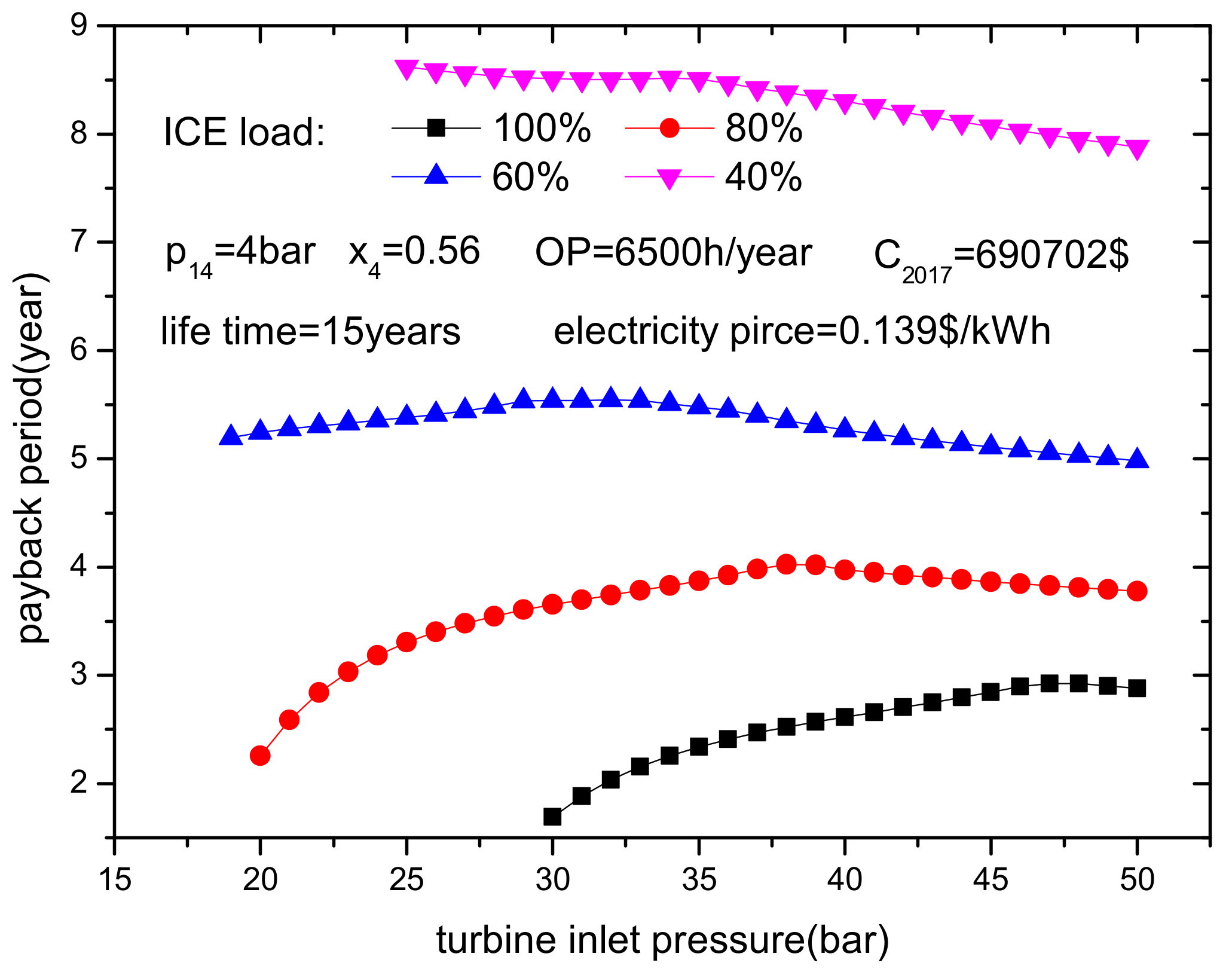
4.2.2. Effect of Turbine Inlet Pressure

As shown in Figure 7, the mass flow rate of the ammonia-water vapor (m₇) changes slightly with the turbine inlet pressure when the mass fraction of the ammonia-water mixture is 0.3. The mass flow rate of the ammonia-water vapor decreases and then increases with turbine inlet pressure when the ammonia mass fraction is 0.4 or 0.5. The enthalpy drop in the turbine increases as turbine inlet pressure increases. Therefore, the net power output of KC increases with an ammonia mass fraction of 0.3 and decreases and subsequently increases with an ammonia mass fraction of 0.4 or 0.5. As shown in Figure 8, the influence of turbine inlet pressure on KC thermal efficiency and the improvement of the thermal efficiency of ICE have similar tendencies with net power output. In short, within the simulation scope of this paper, if the ammonia mass fraction is below 0.34, higher turbine inlet pressures are better. If the ammonia mass fraction is greater than 0.34, a lower turbine inlet pressure is better.

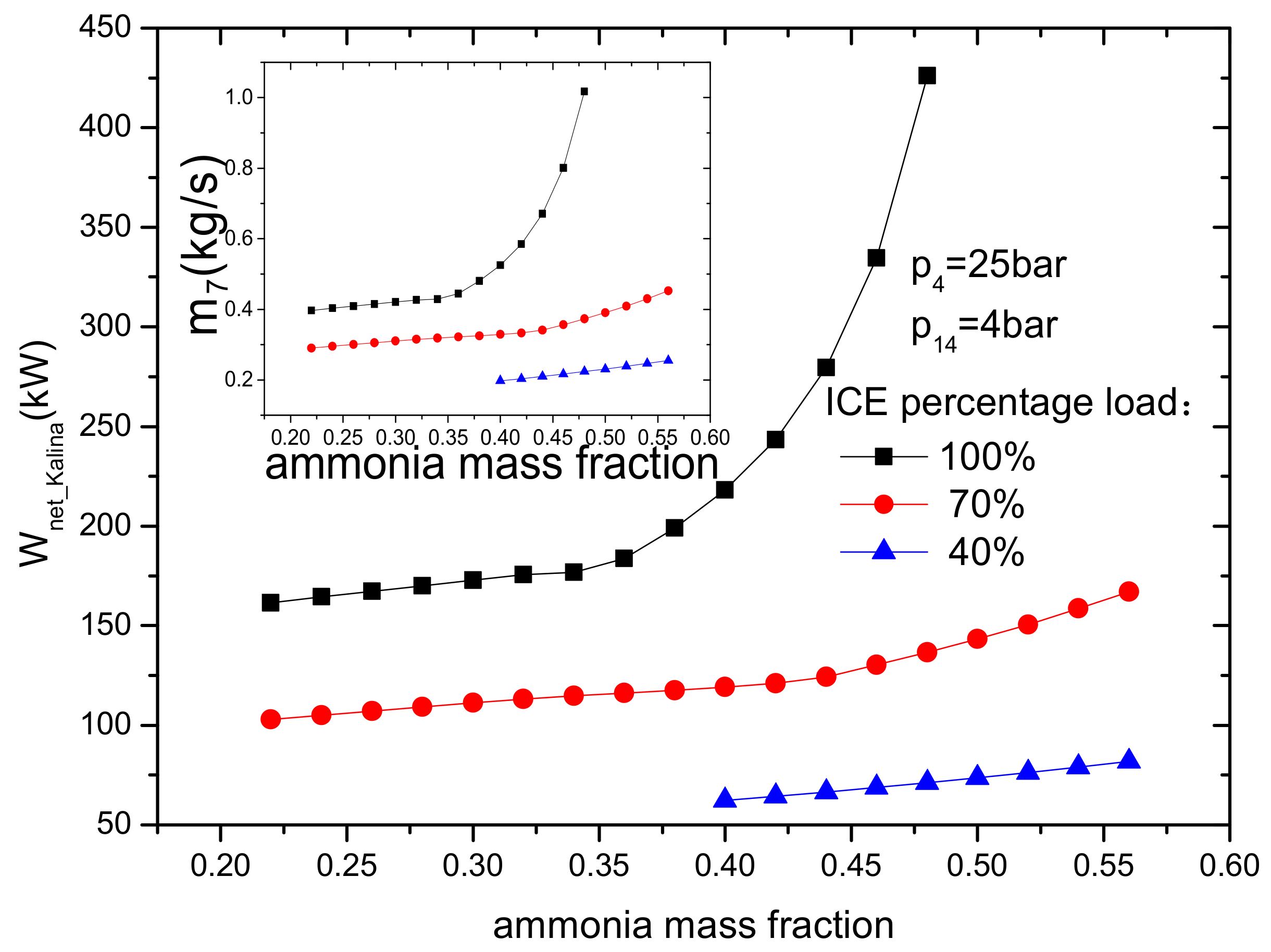
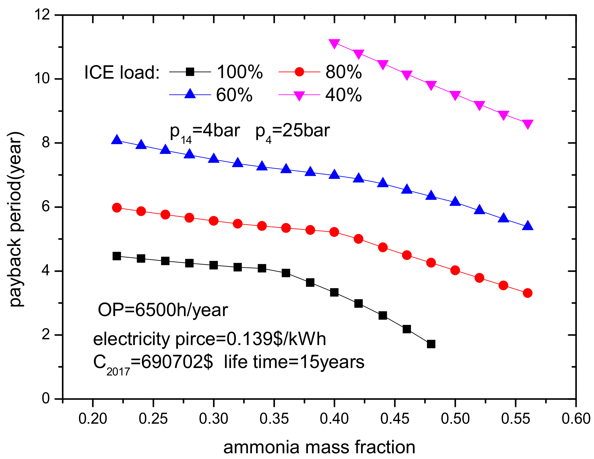
4.2.3. Effect of Ammonia Mass Fraction

Figure 9 and Figure 10 reveal that net power output, KC thermal efficiency and the improvement of the thermal efficiency of ICE benefit from an increased ammonia mass fraction. This finding is observed because the higher the ammonia mass fraction is, the greater the enthalpy drop of the vapor and the vapor flow rate expanding in the turbine is. The improvement of the thermal efficiency of ICE also increases with increased ammonia mass fraction. However, if the ammonia mass fraction is too high, the pump power consumption will increase greatly because the ammonia liquid mixture at the outlet of the condenser (state 14) will turn into a vapor–liquid mixture. This leads to great increase of the work consumption in the pump.

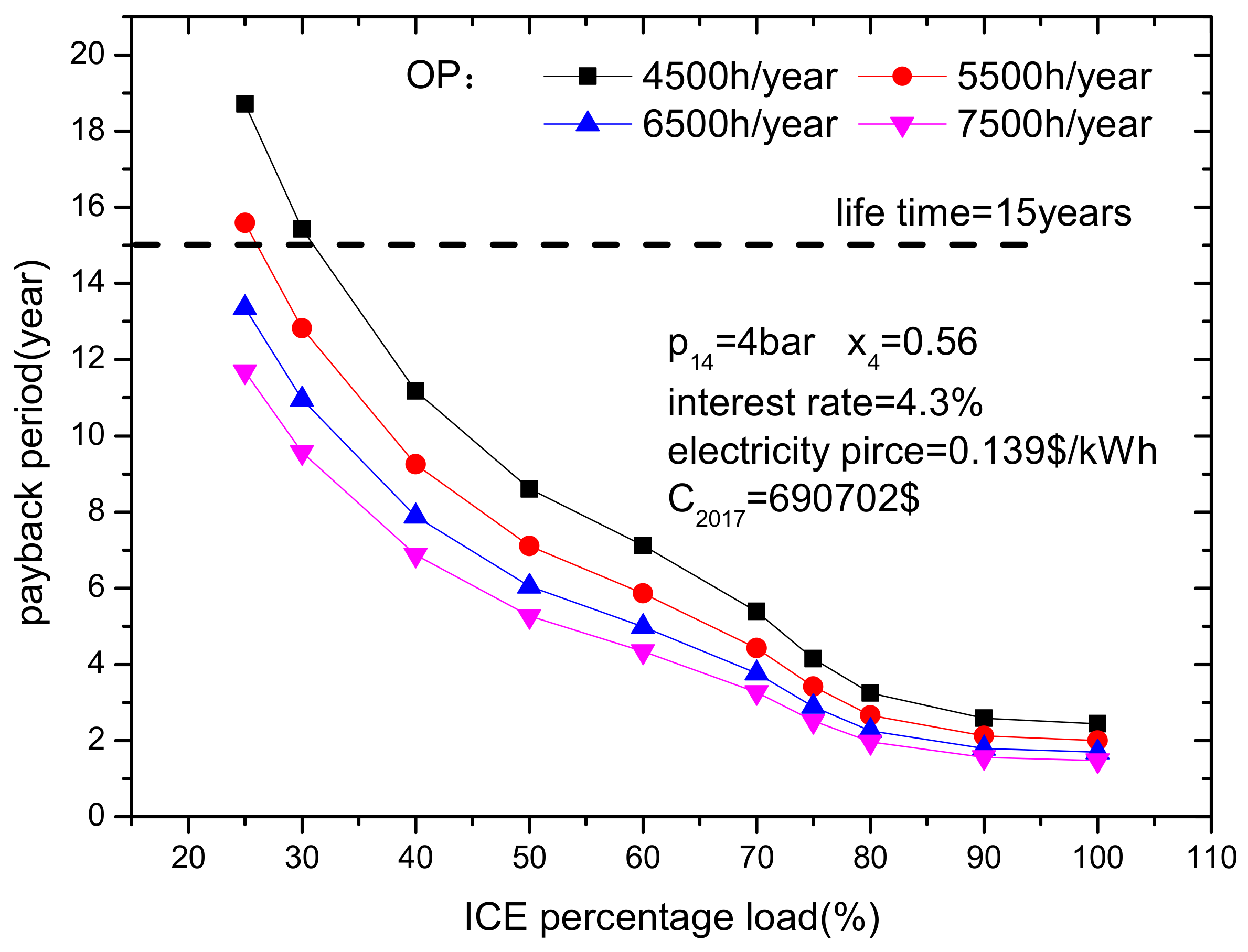
4.3. Economic Performance

By increasing ICE load, the equipment capital investment increases due to a larger heat transfer area. Therefore, the Kalina subsystem has the largest capital investment C₂₀₁₇ at 100% ICE load with an ammonia mass fraction of 0.56 and turbine inlet pressure of 30 bar. If the largest investment (C₂₀₁₇) is taken as the investment of the Kalina subsystem at all loads, the effects of ICE load, turbine inlet pressure and ammonia mass fraction on the payback period are analyzed.

As shown in Figure 11, the minimum payback period decreases with ICE percentage load. This finding is observed because when the equipment investment remains fixed, a higher ICE load leads to more power output and a shorter payback period. The minimum payback periods are 2.44 years, 2.00 years, 1.69 years and 1.47 years at 100% ICE load with annual operation times of 4500 h, 5500 h, 6500 h and 7500 h, respectively. The maximum payback periods are 18.71 years, 15.59 years, 13.36 years and 11.69 years at 25% ICE load with annual operation times of 4500 h, 5500 h, 6500 h and 7500 h, respectively. The minimum payback period of the Kalina subsystem is shorter than the lifetime of 15 years when ICE percentage load is not below 30% and the annual operation times is not below 4500 h. This means that if ICE does not often runs at low loads, the Kalina subsystem can recover the capital investment over the lifetime of the equipment.

The variations of payback period with turbine inlet pressure are presented in Figure 12. Payback period increases and later decreases with turbine inlet pressure if ICE load is not less than 60%. When ICE loads are 100% and 80%, the minimum payback periods are 1.69 years and 2.26 years, respectively, when the turbine inlet pressures are 30 bar and 20 bar, respectively. When ICE loads are 60% and 40%, the minimum payback periods are 5.20 years and 8.62 years, respectively, at a turbine inlet pressure of 50 bar. In short, if the ICE load is high, for example, not less than 70% with an ammonia mass fraction of 0.56, a lower turbine inlet pressure is better for reducing the payback period.

Figure 13 shows that payback period decreases with ammonia mass fraction. This means that a high ammonia mass fraction is good for improving the economic performance of the Kalina subsystem. If the capital investment is fixed, a higher ammonia mass fraction will lead to higher net power output and a shorter payback period. When ICE load is 100%, 80%, 60% and 40%, the minimum payback periods are 1.72 years, 3.30 years, 5.38 years and 8.62 years, respectively.

Figure 14 shows the variation of payback period with annual operation time. Payback period decreases with increasing annual operation time. If annual operation time increases from 3700 h to 8500 h, the decrease of payback period is from 54% to 56% at all ICE loads. This means that annual operation time is a sensible and key parameter to estimate payback period. According to the calculation, payback period is less than 15 years when ICE load does not go below 40%. Figure 15 shows the influence of interest rate on payback period. Higher interest rates result in longer payback periods. When interest rate increases from 2.2% to 8%, the increase of the payback period is from 5.5% to 6%. This finding means that the influence of interest rate on payback period is relatively small.

5. Conclusions

In this paper, a Kalina cycle (KC) with a superheater is used as a bottoming cycle to recover the waste heat from an internal combustion engine (ICE). The thermodynamic and economic analyses are conducted for this bottoming KC. The following conclusions are obtained:

(1)

KC with a superheater is a promising cycle for waste heat recovery from ICE. The Kalina subsystem not only yields extra power output without extra petroleum consumption but also reduces the emissions of CO₂. The maximum net power output and thermal efficiency of KC in this paper are greater than those in the published literature for all ICE loads, and the maximum exergy efficiency is greater than that in the published literature when the ICE load is greater than 40%.

(2)

The net power output, KC thermal efficiency and the improvement of the thermal efficiency of ICE increase with ICE percentage load and ammonia mass fraction. Compared with the single ICE, the increase of thermal efficiency is approximately 21.6% at 100% ICE percentage load. In addition, within the scope of this paper, if the ammonia mass fraction is below 0.34, a higher turbine inlet pressure is better for improving thermal performance. If the ammonia mass fraction is greater than 0.34, a lower turbine inlet pressure is better.

(3)

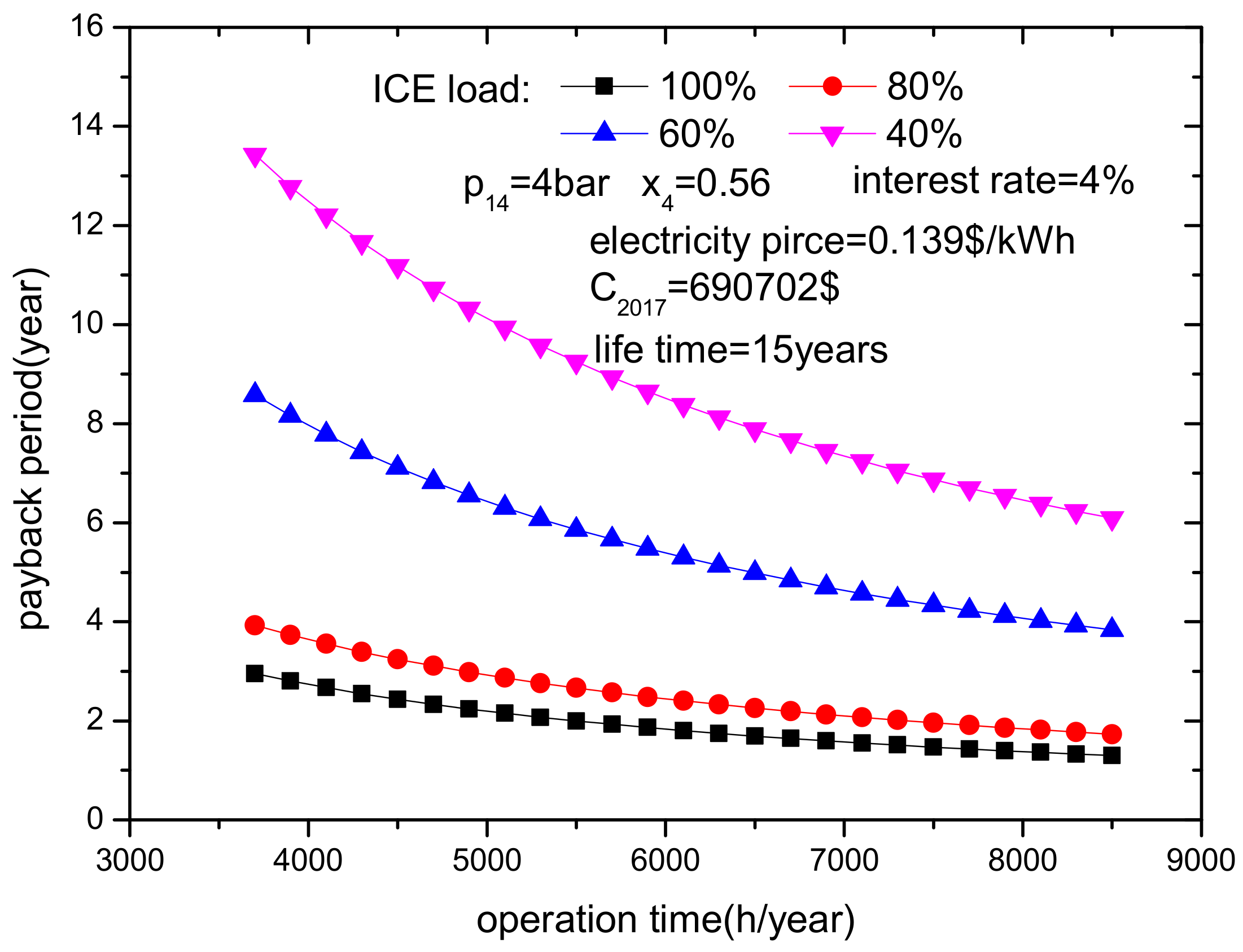
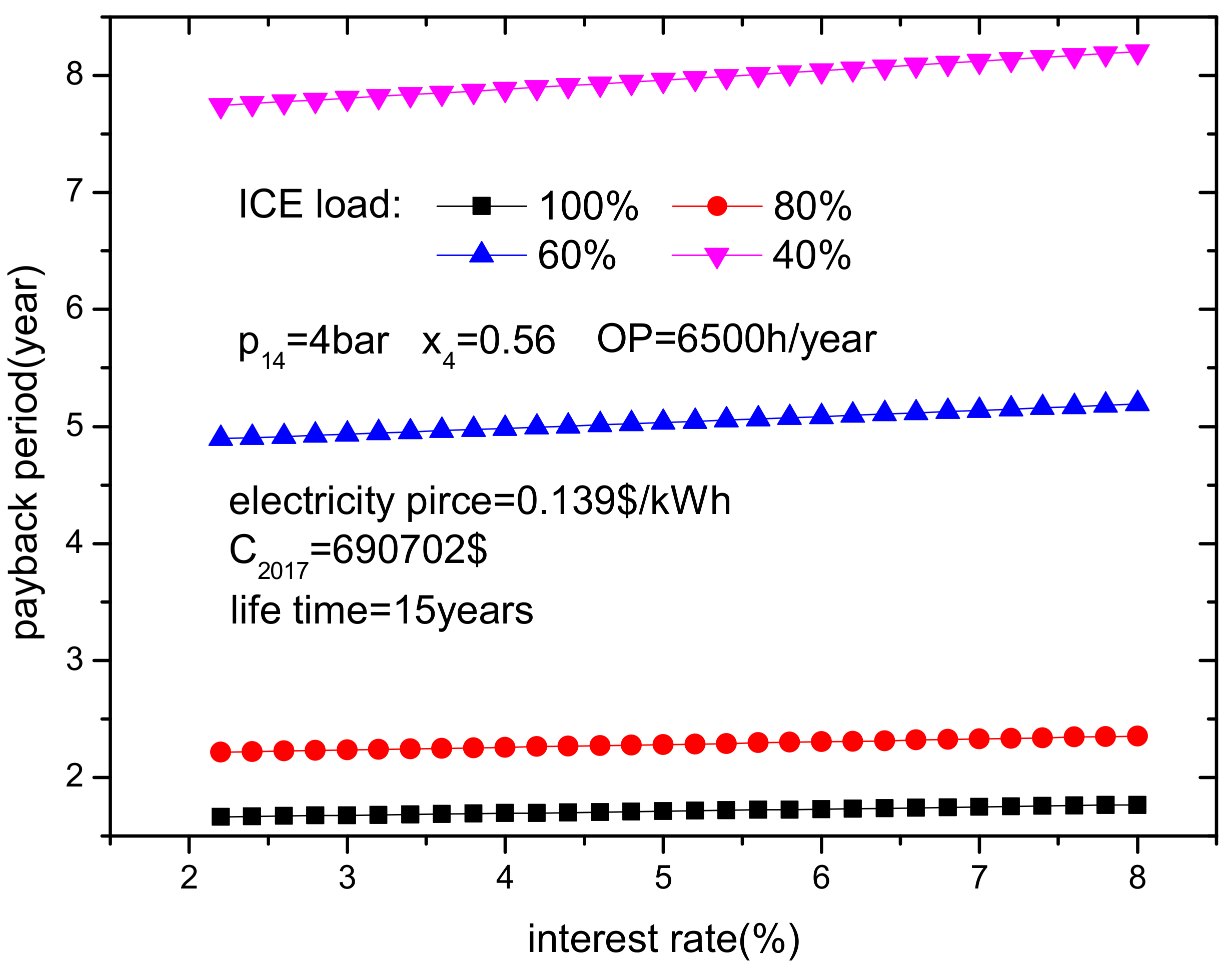
The capital investment increases with ICE load because a high ICE load results in a high heat transfer area. It is assumed that the Kalina subsystem that requires the largest investment (C₂₀₁₇), is used at all ICE loads in the paper. Both higher ICE loads and higher ammonia mass fractions result in shorter payback periods. If ICE load is high, a lower turbine inlet pressure is better for reducing the payback period. In addition, both longer annual operation times and lower interest rates lead to shorter payback periods. However, it is worth noting that the payback period will be longer than the ICE lifetime if the ICE load is too low and the annual operation time is too short.

References

1. Wei, M.; Fang, J.; Ma, C.; Danish, S.N. Waste heat recovery from heavy-duty diesel engine exhaust gases by medium temperature orc system. Sci. China Technol. Sci. 2011, 54, 2746–2753. [Google Scholar] [CrossRef]
2. Zhu, S.; Deng, K.; Qu, S. Energy and exergy analyses of a bottoming Rankine cycle for engine exhaust heat recovery. Energy 2013, 58, 448–457. [Google Scholar] [CrossRef]
3. Kostowski, W.J.; Usón, S. Comparative evaluation of a natural gas expansion plant integrated with an IC engine and an organic rankine cycle. Energy Convers. Manag. 2013, 75, 509–516. [Google Scholar] [CrossRef]
4. Seyedkavoosi, S.; Javan, S.; Kota, K. Exergy-based optimization of an organic Rankine cycle (ORC) for waste heat recovery from an internal combustion engine (ICE). Appl. Therm. Eng. 2017, 126, 447–457. [Google Scholar] [CrossRef]
5. Wang, X.; Shu, G.; Tian, H.; Liu, P.; Li, X.; Jing, D. Engine working condition effects on the dynamic response of organic Rankine cycle as exhaust waste heat recovery system. Appl. Therm. Eng. 2017, 123, 670–681. [Google Scholar] [CrossRef]
6. Pili, R.; Pastrana, J.D.C.; Romagnoli, A.; Spliethoff, H.; Wieland, C. Working fluid selection and optimal power-to-weight ratio for orc in long-haul trucks. Energy Procedia 2017, 129, 754–761. [Google Scholar] [CrossRef]
7. Wang, E.; Yu, Z.; Zhang, H.; Yang, F. A regenerative supercritical-subcritical dual-loop organic Rankine cycle system for energy recovery from the waste heat of internal combustion engines. Appl. Energy 2017, 190, 574–590. [Google Scholar] [CrossRef]
8. Scaccabarozzi, R.; Tavano, M.; Invernizzi, C.M.; Martelli, E. Thermodynamic Optimization of heat recovery ORCs for heavy duty Internal Combustion Engine: Pure fluids vs. zeotropic mixtures. Energy Procedia 2017, 129, 168–175. [Google Scholar] [CrossRef]
9. Liu, P.; Shu, G.; Tian, H.; Wang, X. Engine Load Effects on the Energy and Exergy Performance of a Medium Cycle/Organic Rankine Cycle for Exhaust Waste Heat Recovery. Entropy 2018, 20, 1–23. [Google Scholar]
10. Wang, X.; Shu, G.; Tian, H.; Liu, P.; Jing, D.; Li, X. Dynamic analysis of the dual-loop Organic Rankine Cycle for waste heat recovery of a natural gas engine. Energy Convers. Manag. 2017, 148, 724–736. [Google Scholar] [CrossRef]
11. Kalina, A.I. Combined-cycle system with novel bottoming cycle. J. Eng. Gas Turbines Power 1984, 106, 737–742. [Google Scholar] [CrossRef]
12. Ibrahim, O.; Klein, S. Absorption power cycles. Energy 1996, 21, 21–27. [Google Scholar] [CrossRef]
13. Fu, W.; Zhu, J.; Zhang, W.; Lu, Z. Performance evaluation of Kalina cycle subsystem on geothermal power generation in the oilfield. Appl. Therm. Eng. 2013, 54, 497–506. [Google Scholar] [CrossRef]
14. Madhawa Hettiarachchi, H.D.; Golubovic, M.; Worek, W.M.; Ikegami, Y. The performance of the kalina cycle system 11(kcs-11) with low-temperature heat sources. J. Energy Resour. Technol. 2007, 129, 243–247. [Google Scholar] [CrossRef]
15. Singh, O.K.; Kaushik, S.C. Energy and exergy analysis and optimization of Kalina cycle coupled with a coal fired steam power plant. Appl. Therm. Eng. 2013, 51, 787–800. [Google Scholar] [CrossRef]
16. Li, S.; Dai, Y. Thermo-economic comparison of kalina and CO2 transcritical power cycle for low temperature geothermal sources in China. Appl. Therm. Eng. 2014, 70, 139–152. [Google Scholar] [CrossRef]
17. Yari, M.; Mehr, A.S.; Zare, V.; Mahmoudi, S.M.S.; Rosen, M.A. Exergoeconomic comparison of TLC (trilateral rankine cycle), ORC (organic rankine cycle) and Kalina cycle using a low grade heat source. Energy 2015, 83, 712–722. [Google Scholar] [CrossRef]
18. Wang, E.; Yu, Z. A numerical analysis of a composition-adjustable Kalina cycle power plant for power generation from low-temperature geothermal sources. Appl. Energy 2016, 180, 834–848. [Google Scholar] [CrossRef]
19. Fallah, M.; Mahmoudi, S.M.S.; Yari, M.; Akbarpour Ghiasi, R. Advanced exergy analysis of the Kalina cycle applied for low temperature enhanced geothermal system. Energy Convers. Manag. 2016, 108, 190–201. [Google Scholar] [CrossRef]
20. Nemati, A.; Nami, H.; Ranjbar, F.; Yari, M. A comparative thermodynamic analysis of ORC and Kalina cycles for waste heat recovery: A case study for CGAM cogeneration system. Case Stud. Therm. Eng. 2017, 9, 1–13. [Google Scholar] [CrossRef]
21. Gharde, P.R.; Sali, N.V. Design of Kalina cycle for waste heat recovery from 1196 cc multi-cylinder petrol engine. Int. J. Adv. Res. Sci. Eng. 2015, 4, 75–84. [Google Scholar]
22. Yue, C.; Han, D.; Pu, W.; He, W. Comparative analysis of a bottoming transcritical orc and a Kalina cycle for engine exhaust heat recovery. Energy Convers. Manag. 2015, 89, 764–774. [Google Scholar] [CrossRef]
23. Xu, F.; Goswami, D.Y.; Bhagwat, S.S. A combined power/cooling cycle. Energy 2000, 25, 233–246. [Google Scholar] [CrossRef]
24. Madhawa Hettiarachchi, H.D.; Golubovic, M.; Worek, W.M.; Ikegami, Y. Optimum design criteria for an organic Rankine cycle using low-temperature geothermal heat sources. Energy 2007, 32, 1698–1706. [Google Scholar] [CrossRef]
25. Zhang, S.; Wang, H.; Guo, T. Performance comparison and parametric optimization of subcritical Organic Rankine Cycle (ORC) and transcritical power cycle system for low-temperature geothermal power generation. Appl. Energy 2011, 88, 2740–2754. [Google Scholar] [CrossRef]
26. Zhu, Y.; Qu, W.; Yu, P. Chemical Equipment Design Manual; Chemical Industry Press: Beijing, China, 2005. [Google Scholar]
27. Qian, S. Heat Exchanger Design Handbook; Chemical Industry Press: Beijing, China, 2002. [Google Scholar]
28. Rodríguez, C.E.C.; Palacio, J.C.E.; Venturini, O.J.; Lora, E.E.S.; Cobas, V.M.; dos Santos, D.M.; Dotto, F.R.L.; Gialluca, V. Exergetic and economic analysis of Kalina cycle for low temperature geothermal sources in Brazil. Appl. Therm. Eng. 2013, 52, 109–119. [Google Scholar] [CrossRef]
29. Bahlouli, K.; Khoshbakhti Saray, R.; Sarabchi, N. Parametric investigation and thermo-economic multi-objective optimization of an ammonia–water power/cooling cycle coupled with an HCCI (homogeneous charge compression ignition) engine. Energy 2015, 86, 672–684. [Google Scholar] [CrossRef]
30. Xia, J.; Wang, J.; Lou, J.; Zhao, P.; Dai, Y. Thermo-economic analysis and optimization of a combined cooling and power (CCP) system for engine waste heat recovery. Energy Convers. Manag. 2016, 128, 303–316. [Google Scholar] [CrossRef]
31. Chemical Enineering. Available online: http://www.chemengonline.com/cepci-updates-january-2018-prelim-and-december-2017-final/ (accessed on 24 March 2018).
32. Chen, Y.; Han, W.; Jin, H. Investigation of an ammonia-water combined power and cooling system driven by the jacket water and exhaust gas heat of an Internal combustion engine. Int. J. Refrig. 2017, 82, 174–188. [Google Scholar] [CrossRef]
33. Wang, X.Q.; Li, X.P.; Li, Y.R.; Wu, C.M. Payback period estimation and parameter optimization of subcritical organic Rankine cycle system for waste heat recovery. Energy 2015, 88, 734–745. [Google Scholar] [CrossRef]
34. State Grid. Available online: http://www.95598.cn/person/sas/es/expenses.jsp?partNo=PM06003001 (accessed on 30 August 2018).
35. De Oliveira Neto, R.; Sotomonte, C.A.R.; Coronado, C.J.; Nascimento, M.A. Technical and economic analyses of waste heat energy recovery from internal combustion engines by the Organic Rankine Cycle. Energy Convers. Manag. 2016, 129, 168–179. [Google Scholar] [CrossRef]
36. Yamaguchi, H.; Zhang, X.R.; Fujima, K.; Enomoto, M.; Sawada, N. Solar energy powered Rankine cycle using supercritical CO2. Appl. Therm. Eng. 2006, 26, 2345–2354. [Google Scholar] [CrossRef]
Figure 1. Schematic of bottoming KC with a superheater for ICE waste heat recovery.
Energies 11 03044 g001
Figure 2. Effects of ICE percentage load on T7 and m7.
Energies 11 03044 g002
Figure 3. Effects of ICE percentage load on ηex_evp, η ex_sup and ηex_Kalina.
Energies 11 03044 g003
Figure 4. Effects of ICE percentage load on Wnet_Kalina and Wnet.
Energies 11 03044 g004
Figure 5. Effects of ICE percentage load on ηt_Kalina, ηt and Δηt.
Energies 11 03044 g005
Figure 6. Maximum ηt_Kalina, ηt, Δηt and ηex_Kalina at different ICE percentage loads.
Energies 11 03044 g006
Figure 7. Effects of turbine inlet pressure on Wnet_Kalina.
Energies 11 03044 g007
Figure 8. Effects of turbine inlet pressure on Δηt.
Energies 11 03044 g008
Figure 9. Effects of ammonia mass fraction on Wnet_Kalina.
Energies 11 03044 g009
Figure 10. Effects of ammonia mass fraction on Δηt.
Energies 11 03044 g010
Figure 11. Minimum payback period at different ICE percentage loads.
Energies 11 03044 g011
Figure 12. Effects of turbine inlet pressure on payback period.
Energies 11 03044 g012
Figure 13. Effects of ammonia mass fraction on payback period.
Energies 11 03044 g013
Figure 14. Effects of annual operation time on payback period.
Energies 11 03044 g014
Figure 15. Effects of interest rate on payback period.
Energies 11 03044 g015