Distributionally Robust Distributed Generation Hosting Capacity Assessment in Distribution Systems

Abstract

Uncertainties associated with the loads and the output power of distributed generations create challenges in quantifying the integration limits of distributed generations in distribution networks, i.e., hosting capacity. To address this, we propose a distributionally robust optimization-based method to determine the hosting capacity considering the voltage rise, thermal capacity of the feeders and short circuit level constraints. In the proposed method, the uncertain variables are modeled as stochastic variables following ambiguous distributions defined based on the historical data. The distributionally robust optimization model guarantees that the probability of the constraint violation does not exceed a given risk level, which can control robustness of the solution. To solve the distributionally robust optimization model of the hosting capacity, we reformulated it as a joint chance constrained problem, which is solved using the sample average approximation technique. To demonstrate the efficacy of the proposed method, a modified IEEE 33-bus distribution system is used as the test-bed. Simulation results demonstrate how the sample size of historical data affects the hosting capacity. Furthermore, using the proposed method, the impact of electric vehicles aggregated demand and charging stations are investigated on the hosting capacity of different distributed generation technologies.

1. Introduction

In recent years, integration of renewable-based distributed generations (DGs) has significantly increased in distribution networks. This is mainly due to governmental support, advancement in technology and economy of scale. Although financially DGs are one of the most viable options for end users, technically, high penetration of them may introduce many issues such as over-voltage, overloading of the feeders [1], degradation of power quality and even higher losses in some situations [2]. These issues limit the integration of DGs in distribution systems. Thus, a hosting capacity (HC) assessment is required prior to the practical deployment of DGs. By doing so, distribution system operators (DSOs) can identify the maximum DG capacity that can be accommodated in their networks and make optimal decisions regarding the placement and sizing of DGs. Furthermore, DSOs can plan the future network augmentation and operation strategies to increase the HC of their system.

The HC problem has been studied considering different constraints [1,2,3,4,5,6,7,8,9,10,11,12,13,14,15]. In [3,4], optimal power flow methods were proposed to solve the HC problem. Analytical [5,6], heuristic [7,8], and sequential power flow-based methods [9,10] were also developed to determine the HC. Nonetheless, the uncertainties related to loads, output power of DGs and the impact of electric vehicles (EVs) were not considered in those studies. The sensitivity of the HC to uncertainties is assessed in [16] using an optimization-based Monte Carlo framework. That study, however, used the time series simulations to address the uncertainties, which can be time consuming for analyzing large numbers of future grid scenarios. To address the uncertainties associated with DGs and loads, an optimization-based framework was presented in [11], which probabilistically assesses the HC. The study in [12] presented a framework to assess the effects of EVs and photovoltaic (PV) systems on the HC, separately.

Two dominant approaches that have been used to model the uncertainties in the HC assessment are (i) the robust optimization (RO) [2,13] and (ii) the stochastic optimization (SO) [14]. In RO approach, the probability distribution functions (PDFs) of uncertainties are not required, and the only necessary data are the boundaries of the uncertain variables. Furthermore, the decisions are made based on the worst-case scenarios in the predefined uncertainty intervals, which result in a conservative solution. In SO-based approach, the uncertainties are considered as random variables with given PDFs. Since obtaining the exact PDFs of uncertain variables is impossible, the robustness of the obtained solution cannot be guaranteed.

In practice, historical data can present more information than the boundaries of uncertain variables. However, historical data can be used to obtain an empirical PDF, not the exact PDF for the uncertain variable. To cope with such cases, distributionally robust optimization (DRO) has been recently developed. In DRO, it is supposed that the exact PDFs of uncertain variables are not available. However, it is supposed that the PDFs of uncertainties are in a confidence set. The confidence set can be constructed using the distributional information of uncertain variables, which is derived from the historical data. For instance, the confidence set can consist of all the PDFs with common mean and covariance matrix [15]. In recent years, DRO have been applied to some power system optimization problems including unit commitment [17], and reserve scheduling [18]. However, those studies often considered the first- and second-order moments of historical data to build the confidence set. Furthermore, all those studies neglected the empirical distribution of uncertainties.

In this paper, we propose a DRO-based method for evaluating the HC in distribution networks. The main contributions of this study are summarized as follows:

• We propose a DRO-based method to evaluate the HC of distribution networks considering uncertainties associated with loads and DGs’ output powers. As the statistic information (i.e., the first- and second-order moments) and the empirical distribution of uncertain variables are exploited in the assessment process, the results of the proposed method are practical and less conservative than those of the RO-based method. To the best of our knowledge, there is no such DRO application in power system that exploit both the statistic information and the empirical distribution simultaneously.
• In the proposed DRO-based method, a risk level is defined to control the robustness, enabling a trade-off between robustness and conservativeness. Unlike the robust optimization, tuning the risk level in the proposed method has a precise physical meaning, i.e., guaranteeing that the probability of operational constraints violation does not exceed a given risk threshold.
• The aggregated EVs and charging stations’ loads are modeled in the HC problem and their effects on the HC have been assessed. To the best of our knowledge, there is no such study that assesses the effect of aggregated EVs and charging stations’ loads on the HC of various types of DGs, i.e., PV, wind, and biomass.

The proposed method is examined on a modified IEEE 33-bus system and the sensitivity of the HC to the DG technology, the EVs aggregate load, the load of EVs charging station and historical data has been assessed.

The reminder of this paper is organized as follows: Section 2 formulates the problem. Section 3 presents the uncertainty modeling. In Section 4, the solution methodology is described. First, the DRO model is transformed into a joint chance constraint (JCC) problem. Then, a solution for the corresponding JCC is introduced. Section 5 presents the numerical results and discussion. Finally, the major conclusions are summarized in Section 6.

2. Mathematical Modeling

The HC is defined as the maximum DG capacity that can be installed in a system without violating its technical constraints irrespective of DGs’ locations. This implies that DGs’ locations should not be defined as independent variables in the optimization model. This, however, raises a question on how to address the uncertainty associated with DGs’ locations in the HC problem. This can be tackled using the HC calculation framework shown in Figure 1. As it can be seen, it is required to generate a large number of location combinations for DGs. Then, the maximum DG capacity for different location scenarios can be identified using the mathematical model. Finally, the minimum of the identified DG capacities for all location scenarios is defined as the actual HC. The focus of this paper is to develop a mathematical model to find the maximum DG capacity for any sets of DG locations. The objective function of this model is presented as follows:

$$\begin{array}{c}\underset{Ca{p}_j^{\mathrm{g}}}{\mathrm{minimize}}\sum _{j\in \mathcal{DG}}-Ca{p}_j^{\mathrm{g}}\hfill \end{array}$$

(1)

where, $\mathcal{DG}$ is the set of buses that have DGs, and $Ca{p}_j^{\mathrm{g}}$ denotes the installed DG capacity at bus (j). The system operation constraints are presented in Section 2.1 and Section 2.2.

2.1. Distribution System Model

Consider a radial network, where $\mathcal{N}=\{0,\cdots ,N_{Bus}\}$ denotes the set of buses. Let $\mathcal{B}$ represents the set of all branches and $(i,j)$ or $i⟶j$ as a branch from bus (i) to bus (j) in the set $\mathcal{B}$. Let $\Gamma$ denotes the set of time periods. For every bus $i\in \mathcal{N}$ and for all $t\in \Gamma$, let $V_{i,t}$ denotes the complex voltage, where ${\upsilon }_{i,t}={\left|V_{i,t}\right|}^2$. Let $s_{i,t}^{\mathrm{d}}=p_{i,t}^{\mathrm{d}}+i{q}_{i,t}^{\mathrm{d}}$ represents the load at bus (i) at time (t). For every line $(i,j)\in \mathcal{B}$ and for all $t\in \Gamma$, $z_{ij}=r_{ij}+i{x}_{ij}$ denotes the complex impedance, $S_{ij,t}=P_{ij,t}+i{Q}_{ij,t}$ denotes the sending-end complex power from bus (i) to bus (j), and $I_{ij,t}$ defines the sending-end complex current from bus (i) to bus (j). Let $s_{i,t}^{\mathrm{g}}=p_{i,t}^{\mathrm{g}}+i{q}_{i,t}^{\mathrm{g}}$ denotes the generation complex power at bus (i) at time (t), and $s_{i,t}^{\mathrm{EV}}=p_{i,t}^{\mathrm{EV}}+i{q}_{i,t}^{\mathrm{EV}}$ represents the EV aggregated complex demand at bus (i) at time (t). For every bus $i\in \mathcal{DG}$, ${\eta }_{i,t}^{\mathrm{g}}$ represents the efficiency factor at time period (t). Assume ${\mathbb{T}}_j$ as the subtree rooted at bus (j) (including (j)). We use $k\in {\mathbb{T}}_j$ to refer to bus (k) in subtree ${\mathbb{T}}_j$ and $(k,l)\in {\mathbb{T}}_j$ to refer to line ($k,l$) in subtree ${\mathbb{T}}_j$. Let ${\mathbb{P}}_j$ defines the set of lines on the path from substation to bus (j). The following equation can be written based on the Ohm’s law:

$$V_{i,t}-V_{j,t}=z_{ij}{I}_{ij,t},\forall (i,j)\in \mathcal{B},\forall t\in \Gamma$$

(2)

taking the magnitude squared from (2) (by taking the product of each side of (2) with its conjugate) results in:

$${\upsilon }_{j,t}={\upsilon }_{i,t}-2(r_{ij}{P}_{ij,t}+x_{ij}{Q}_{ij,t})+{\left|z_{ij}\right|}^2\frac{P_{ij,t}^2+Q_{ij,t}^2}{{\upsilon }_{i,t}},\forall (i,j)\in \mathcal{B},\forall t\in \Gamma$$

(3)

and according to the nodal power balance equations, we have:

$$P_{ij,t}=\sum _{k:j⟶k}{P}_{jk,t}+p_{j,t}^{\mathrm{d}}-p_{j,t}^{\mathrm{g}}+p_{j,t}^{\mathrm{EV}}+r_{ij}\frac{P_{ij,t}^2+Q_{ij,t}^2}{{\upsilon }_i},\forall j\in \mathcal{N},\forall t\in \Gamma$$

(4)

$$Q_{ij,t}=\sum _{k:j⟶k}{Q}_{jk,t}+q_{j,t}^{\mathrm{d}}-q_{j,t}^{\mathrm{g}}+q_{j,t}^{\mathrm{EV}}+x_{ij}\frac{P_{ij,t}^2+Q_{ij,t}^2}{{\upsilon }_{i,t}},\forall j\in \mathcal{N},\forall t\in \Gamma$$

(5)

$$\left\{\begin{array}{c}{p}_{i,t}^{\mathrm{g}}={\eta }_{i,t}^{\mathrm{g}}Ca{p}_i^{\mathrm{g}},\hfill \\ q_{i,t}^{\mathrm{g}}=tan\left({\varphi }_{i,t}\right)p_{i,t}^{\mathrm{g}},\hfill \end{array}\right.\forall i\in \mathcal{DG},\forall t\in \Gamma$$

(6)

where, ${\varphi }_{i,t}$ is the power factor angle at bus (i) at time period (t). Considering the unique path from the substation to each bus, the voltage at bus (j) can be calculated as follows:

$${\upsilon }_{j,t}={\upsilon }_{0,t}-\sum _{(l,k)\in {\mathbb{P}}_j}2(r_{lk}{P}_{lk,t}+x_{lk}{Q}_{lk,t})+\sum _{(l,k)\in {\mathbb{P}}_j}{\left|z_{lk}\right|}^2\frac{P_{lk,t}^2+Q_{lk,t}^2}{{\upsilon }_{l,t}},\forall j\in \mathcal{N},\forall t\in \Gamma$$

(7)

The quadratic terms in (4), (5) and (7) are the sources of non-convexity in the optimization problem (1). These terms are small and ignoring them in the HC problem results in a sufficiently accurate linear model [15,19]. Therefore, equations (4), (5) and (7) can be written as:

$$P_{ij,t}=\sum _{k:j⟶k}{P}_{jk,t}+p_{j,t}^{\mathrm{d}}-p_{j,t}^{\mathrm{g}}+p_{j,t}^{\mathrm{EV}},\forall j\in \mathcal{N},\forall t\in \Gamma$$

(8)

$$Q_{ij,t}=\sum _{k:j⟶k}{Q}_{jk,t}+q_{j,t}^{\mathrm{d}}-q_{j,t}^{\mathrm{g}}+q_{j,t}^{\mathrm{EV}},\forall j\in \mathcal{N},\forall t\in \Gamma$$

(9)

$${\upsilon }_{j,t}={\upsilon }_{0,t}-\sum _{(l,k)\in {\mathbb{P}}_j}2(r_{lk}{P}_{lk,t}+x_{lk}{Q}_{lk,t}),\forall j\in \mathcal{N},\forall t\in \Gamma$$

(10)

2.2. Technical Constraints

The following technical constraints are considered for determining the HC:

2.2.1. Steady State Voltage Constraint

$$\underline{{\upsilon }_i}\le {\upsilon }_{i,t}\le \overline{{\upsilon }_i},\forall i\in \mathcal{N},\forall t\in \Gamma$$

(11)

where, $\underline{{\upsilon }_i}$ and $\overline{{\upsilon }_i}$ are the minimum and maximum voltage limits at bus (i), respectively.

2.2.2. Thermal Capacity Constraints

The apparent power flow of lines and substation transformer is limited by a higher bound as follows:

$$P_{ij,t}^2+Q_{ij,t}^2\le {\overline{\left|S_{ij}\right|}}^2,\forall (i,j)\in \mathcal{B},\forall t\in \Gamma$$

(12)

where, $\overline{\left|S_{ij}\right|}$ is the maximum apparent power of line $(i,j)$. Equation (12) is a quadratic nonlinear constraint, which needs to be linearized to simplify the final problem formulation. For doing so, we rotate the tangent (13) around the original circular constraint (12) using the counter clockwise rotation matrix (14).

$$P_{ij,t}+Q_{ij,t}\le \sqrt{2}\overline{\left|S_{ij}\right|},\forall (i,j)\in \mathcal{B},\forall t\in \Gamma$$

(13)

$$A=\left[\begin{array}{cc}cos\left(\theta \right)& -sin\left(\theta \right)\\ sin\left(\theta \right)& cos\left(\theta \right)\end{array}\right]$$

(14)

where, $\theta$ is the rotation angle. Applying (14) to (13) results in:

$$[cos\left(\theta \right)+sin\left(\theta \right)]P_{ij,t}+[cos\left(\theta \right)-sin\left(\theta \right)]Q_{ij,t}\le \sqrt{2}\overline{\left|S_{ij}\right|},\forall (i,j)\in \mathcal{B},\forall t\in \Gamma$$

(15)

2.2.3. Short Circuit Level (SCL) Constraint

One of the important characteristics of distribution systems is SCL, which is defined as the maximum acceptable fault level. A basic requirement for connecting DGs to the networks is that the SCL in presence of DGs should remain below the designed SCL [20]. It is shown in [21] that the SCL can be modeled as follows:

$$\sum _{j\in \mathcal{DG}}{a}_{j}Ca{p}_j^{\mathrm{g}}+SC{L}_{\mathrm{sub}}\le SC{L}_{\mathrm{Rated}}$$

(16)

where, $a_j$ is the dependency of SCL to the capacity of the DG at bus (j), $SC{L}_{\mathrm{sub}}$ is the SCL at substation without DGs, and $SC{L}_{\mathrm{Rated}}$ is the rated SCL at substation. It is worth mentioning that $a_j$ depends on the structure of the system and the DG type; e.g., $a_j$ is very small for PVs [22].

2.3. Deterministic Problem Formulation Summary

The deterministic HC problem is formulated as follows:

$$\begin{array}{c}\underset{Ca{p}_j^{\mathrm{g}}}{\mathrm{minimize}}\sum _{j\in \mathcal{DG}}-Ca{p}_j^{\mathrm{g}},\hfill \\ \mathrm{s}.\mathrm{t}.\left(6\right),\left(8\right)--\left(10\right),\left(11\right),\left(15\right),\left(16\right)\hfill \end{array}$$

(17)

In practice, the output power of DGs and the loads are uncertain variables and modeling them as deterministic variables is not realistic. Therefore, the HC optimization model should include such uncertainties, as explained in the next subsection.

2.4. Distributionally Robust Optimization (DRO) HC Model

The uncertainties of the DG output ($p_{i,t}^{\mathrm{g}}$), load ($p_{i,t}^{\mathrm{L}}$), and EVs aggregated demand ($p_{i,t}^{\mathrm{EV}}$) at bus (i) are modeled as follows:

$$\left\{\begin{array}{c}{\eta }_{i,t}^{\mathrm{g}}={\widehat{\eta }}_{i,t}^{\mathrm{g}}+{\xi }_{i,t}^{\mathrm{g}}\hfill \\ p_{i,t}^{\mathrm{L}}={\widehat{p}}_{i,t}^{\mathrm{L}}+{\xi }_{i,t}^{\mathrm{L}}\hfill \\ p_{i,t}^{\mathrm{EV}}={\widehat{p}}_{i,t}^{\mathrm{EV}}+{\xi }_{i,t}^{\mathrm{EV}}\hfill \end{array}\right.$$

(18)

where, ${\xi }_{i,t}^{\mathrm{g}}$, ${\xi }_{i,t}^{\mathrm{L}}$, and ${\xi }_{i,t}^{\mathrm{EV}}$ model the prediction error of the DG output, load and aggregated demand of EVs, respectively; ${\widehat{\eta }}_{i,t}^{\mathrm{g}}$, ${\widehat{p}}_{i,t}^{\mathrm{L}}$ and ${\widehat{p}}_{i,t}^{\mathrm{EV}}$ are the predicted values of ${\eta }_{i,t}^{\mathrm{g}}$, $p_{i,t}^{\mathrm{L}}$ and $p_{i,t}^{\mathrm{EV}}$, respectively. Considering the definition of subtree ${\mathbb{T}}_j$, substituting (18) in (6), (8)–(10), and denoting $\xi =\{{\xi }_{i,t}^{\mathrm{g}},{\xi }_{i,t}^{\mathrm{L}},{\xi }_{i,t}^{\mathrm{EV}}\}$ to the vector of uncertain variables, the power flow state variables ($P_{ij,t},Q_{ij,t},{\upsilon }_{j,t}$) can be written as functions of ${\mathit{Cap}}^{\mathrm{g}}$ and $\xi$. Thus, all constraints can be expressed as follows:

$$G_k^{\mathrm{eq}}\left({\mathit{Cap}}^{\mathrm{g}},\xi \right)=0,\forall k\in {\mathcal{C}}^{\mathrm{eq}}$$

(19)

$$G_k\left({\mathit{Cap}}^{\mathrm{g}},\xi \right)\le 0,\forall k\in \mathcal{C}$$

(20)

where, ${\mathcal{C}}^{\mathrm{eq}}$ and $\mathcal{C}$ are the sets of equality and inequality constraints for the HC problem. Hence, the uncertain HC model is presented as follows:

$$\begin{array}{c}\underset{Ca{p}_j^{\mathrm{g}}}{\mathrm{minimize}}\sum _{j\in \mathcal{DG}}-Ca{p}_j^{\mathrm{g}}\hfill \\ \mathrm{s}.\mathrm{t}.\hfill \\ G_k^{\mathrm{eq}}\left({\mathit{Cap}}^{\mathrm{g}},\xi \right)=0,\forall k\in {\mathcal{C}}^{\mathrm{eq}}\hfill \\ G_k\left({\mathit{Cap}}^{\mathrm{g}},\xi \right)\le 0,\forall k\in \mathcal{C}\hfill \end{array}$$

(21)

To immunize the HC model (21) against the uncertainty vector, $\xi$, we adapt a distributionally robust approach. In this approach, a risk level is defined to adjust the conservatism of the solution. From a modeling prospective, the distributionally robust HC problem is defined as follows:

$$\begin{array}{c}\underset{Ca{p}_j^{\mathrm{g}}}{\mathrm{minimize}}\sum _{j\in \mathcal{DG}}-Ca{p}_j^{\mathrm{g}}\hfill \\ \mathrm{s}.\mathrm{t}.\hfill \\ \underset{f\in {\mathcal{D}}_{\varphi }}{\inf }\left\{\underset{\xi \sim f}{\mathrm{Pr}}\left[T\left({\mathit{Cap}}^{\mathrm{g}},\xi \right)\right]\right\}\ge 1-\tau \hfill \end{array}$$

(22)

where, $\tau$ is the risk level, ${\mathcal{D}}_{\varphi }$ is the confidence set, and $T\left({\mathit{Cap}}^{\mathrm{g}},\xi \right)=\left\{\begin{array}{cc}{G}_k^{\mathrm{eq}}\left({\mathit{Cap}}^{\mathrm{g}},\xi \right)=0\hfill & \forall k\in {\mathcal{C}}^{\mathrm{eq}}\hfill \\ G_k\left({\mathit{Cap}}^{\mathrm{g}},\xi \right)\le 0\hfill & \forall k\in \mathcal{C}\hfill \end{array}\right.$. The next step is modeling the uncertainty vector, $\xi$, and the confidence set, ${\mathcal{D}}_{\varphi }$, which is detailed in the next section.

3. Uncertainty Modeling

In this section, the uncertainties associated with the outputs of DGs, loads and aggregated demands of EVs as well as the confidence set are modeled based on the historical data. Herein, the generation technologies are PV, wind, and biomass.

3.1. Uncertainty Modeling of PV Generation

The stochastic variations of PVs from their predicted output values follow a Beta distribution [23]. This distribution, defined by two shape parameters, $\alpha$ and $\beta$, enables us to represent the prediction error of a predicted output power, ${\widehat{p}}_{i,t}^{\mathrm{g}}$, with the normalized predicted output power and a standard deviation, which varies with ${\widehat{\eta }}_{i,t}^{\mathrm{g}}$. The Beta function for modeling the occurrence of an output power, x, if a prediction value, ${\widehat{p}}_{i,t}^{\mathrm{g}}$, has been forecast, is as follows:

$$f_{{\widehat{\eta }}_{i,t}^{\mathrm{g}}}\left(x\right)=x^{\alpha -1}{(1-x)}^{\beta -1}$$

(23)

The shape parameters $\alpha$ and $\beta$ are related to the normalized predicted output power and variance as follows:

$${\widehat{\eta }}_{i,t}^{\mathrm{g}}=\frac{{\widehat{p}}_{i,t}^{\mathrm{g}}}{Ca{p}^{\mathrm{g}}}=\frac{\alpha }{\alpha +\beta }$$

(24)

$${\sigma }^2=\frac{\alpha .\beta }{{(\alpha +\beta )}^2.(\alpha +\beta +1)}$$

(25)

3.2. Uncertainty Modeling of Wind Generation

A Beta function is justified to model the prediction error of the wind power [24]. The relation between the parameters of Beta distribution (i.e., $\alpha$ and $\beta$) and the normalized predicted output power and variance are presented in (24) and (25).

3.3. Uncertainty Modeling of Biomass Generation

The biomass DGs are considered as firm generation. Thus, the output powers of such DGs are considered constant at their rated capacities [25].

3.4. Uncertainty Modeling of Load

Load uncertainty is usually modeled by a normal distribution, in which, the mean value is the forecast load and the standard deviation is set to be 2% of the mean value [26].

3.5. Uncertainty Modeling of EV Demand

The demand of EVs depends on the number of EVs, their state of charge (SOC), charging start time and its duration. These variables are uncertain, so the overall charging demand of EVs is uncertain as well. Considering the charging behavior of EVs, the overall demand can be categorized as follows:

3.5.1. Overall Charging Demand of EVs in a Local Residential Community

It was shown in [27,28] that the aggregated demand of EVs in a residential community follows a normal distribution at each hour, and the average and standard deviation of the distribution depend on the number of EVs and the transportation data of the area.

3.5.2. Overall Charging Demand of an EV Charging Station

The demand of a charging station depends on the number of EVs that arrive in different time intervals, the duration of a charging process and the charging power profile [27,29]. It was shown in [27] that the demand uncertainty of a charging station can be modeled by using a Weibull distribution.

3.6. Modeling the Confidence Set

A challenging difficulty of handling the uncertainties in HC optimization is the accessibility to the exact PDFs. Since the historical data is limited or there might be not much trust in it, assuming the perfect knowledge about the PDFs of uncertainties is unrealistic. To address this, an ambiguity set of distributions can be used. A common method to create an ambiguity set exploiting the empirical distributions is $\varphi -$divergence, which is defined as follows:

$$D_{\varphi }(f\parallel f_0)={\int }_{\Omega }\varphi \left(\frac{f\left(\xi \right)}{f_0\left(\xi \right)}\right)f_0\left(\xi \right)d\xi$$

(26)

where, f and $f_0$ are the actual and estimated density functions, respectively; $\xi \in {\mathbb{R}}^K$ represents a K-dimensional random vector defined on a probability space, $\Omega$, and $\varphi :\mathbb{R}⟶\mathbb{R}$ is a convex function on ${\mathbb{R}}^{+}$. We refer the readers to [30] for more details on characteristics of $\varphi -$divergences. One of the most common used members of the $\varphi -$divergence families is Variation Distance, which is defined as:

$${\varphi }_{\mathrm{VD}}\left(x\right)=\left|x-1\right|forx\ge 0$$

(27)

Based on the $\varphi -$divergences, a confidence set can be built as follows:

$${\mathcal{D}}_{\varphi }=\left\{\mathbb{P}\in {\mathcal{M}}_{+}:D_{\varphi }(f\parallel f_0)\le \psi ,f=d\mathbb{P}/d\xi \right\}$$

(28)

where, ${\mathcal{M}}_{+}$ represents the set of all cumulative density functions (CDFs), and $\psi$ denotes the risk-aversion level. The higher the risk-aversion level ($\psi$) is, the bigger the ambiguity set and the more conservative the result of the optimization model would be. However, as compared to uncertainty sets in the RO or the moment-based ambiguity sets, the confidence set, ${\mathcal{D}}_{\varphi }$, can more accurately depict the profile of PDFs, and so provides a less conservative result.

4. Solution Methodology

To solve the HC problem (22), we convert it to an equivalent JCC optimization by employing a theory presented in [30]. Then, the sample average approximation is used to solve the equivalent JCC [31,32]. Before presenting the equivalent JCC problem, we need to review the definition of conjugate duality. For a given function $g:\mathbb{R}⟶\mathbb{R}$, the conjugate $g^{*}:\mathbb{R}⟶\mathbb{R}\cup \left\{+\infty \right\}$ is defined as follows:

$$g^{*}\left(t\right)=\underset{x\in \mathbb{R}}{\sup }\left\{tx-g\left(x\right)\right\}$$

(29)

Definition 1.

For a convex function $\varphi :\mathbb{R}⟶\mathbb{R}$ that $\varphi \left(1\right)=0$ and $\varphi \left(x\right)=+\infty \forall x<0$, define $\underline{m}\left({\varphi }^{*}\right):=\sup \left\{m\in \mathbb{R}:{\varphi }^{*}is\mathrm{a}finiteconstanton(-\infty ,m]\right\}$ and $\overline{m}\left({\varphi }^{*}\right):=\inf \left\{m\in \mathbb{R}:{\varphi }^{*}\left(m\right)=+\infty \right\}$.

4.1. Equivalent JCC

Let ${\mathbb{P}}_0\left(T\left({\mathit{Cap}}^{\mathrm{g}},\xi \right)\right)$ be the probability distribution defined by estimated PDF $f_0$. Then, the distributionally robust chance constraint, $\underset{f\in {\mathcal{D}}_{\varphi }}{\inf }\left\{\underset{\xi \sim f}{\mathrm{Pr}}\left[T\left({\mathit{Cap}}^{\mathrm{g}},\xi \right)\right]\right\}\ge 1-\tau$, can be reformulated equivalently as a JCC [30] given in (30):

$${\mathbb{P}}_0\left(T\left({\mathit{Cap}}^{\mathrm{g}},\xi \right)\right)\ge 1-{\tau }_{+}^{{}^{\prime }}$$

(30)

where,

$${\tau }^{{}^{\prime }}=1-\underset{\begin{array}{c}z>0,\pi z\le {\ell }_{\varphi }\\ \underline{m}\left({\varphi }^{*}\right)\le z_0+z\le \overline{m}\left({\varphi }^{*}\right)\end{array}}{\inf }\left\{\frac{{\varphi }^{*}(z_0+z)-z_0-\tau z+\psi }{{\varphi }^{*}(z_0+z)-{\varphi }^{*}\left(z_0\right)}\right\}$$

${\tau }_{+}^{{}^{\prime }}=\max \left\{{\tau }^{{}^{\prime }},0\right\}$ for ${\tau }^{{}^{\prime }}\in \mathbb{R}$, ${\ell }_{\varphi }=\underset{x⟶+\infty }{\lim }\left(\frac{\varphi \left(x\right)}{x}\right)$, and

$$\pi =\left\{\begin{array}{cc}-\infty \hfill & Leb\left\{[f_0=0]\right\}=0,\hfill \\ 0\hfill & \begin{array}{c}Leb\left\{[f_0=0]\right\}>0\mathrm{and}\hfill \\ Leb\left\{[f_0=0]\setminus T\left({\mathit{Cap}}^{\mathrm{g}},\xi \right)\right\}=0,\hfill \end{array}\hfill \\ 1\hfill & o.w,\hfill \end{array}\right.$$

where, $Leb\{·\}$ represent the Lebesgue measure on ${\mathbb{R}}^k$ and $[f_0=0]:=\{\xi \in \Omega :f_0\left(\xi \right)=0\}$. For the reformulated distributionally robust HC presented in (30), the value of ${\ell }_{\varphi }$, $\underline{m}\left({\varphi }^{*}\right)$, and $\overline{m}\left({\varphi }^{*}\right)$ for variation distance $\varphi$-divergence is presented in

Table 1. Value of ${\ell }_{\varphi }$, $\underline{m}\left({\varphi }^{*}\right)$, and $\overline{m}\left({\varphi }^{*}\right)$ for variation distance $\varphi$-divergence.

Divergences	${\mathit{\ell }}_{\mathit{\varphi }}$	$\underline{\mathit{m}}\left({\mathit{\varphi }}^{*}\right)$	$\overline{\mathit{m}}\left({\mathit{\varphi }}^{*}\right)$
Variation distance	1	-1	1

.

Therefore, if we have a function $\tau ({\tau }_{+}^{{}^{\prime }},\varphi ,\psi )$ that maps the ${\tau }_{+}^{{}^{\prime }}$ to the original risk level, $\tau$, for the given tolerance, $\psi$, and $\varphi$-divergence, it can be stated that if (30) is satisfied by some ${\mathit{Cap}}^{\mathrm{g}}$, then $\underset{f\in {\mathcal{D}}_{\varphi }}{\inf }\left\{\underset{\xi \sim f}{\mathrm{Pr}}\left[T\left({\mathit{Cap}}^{\mathrm{g}},\xi \right)\right]\right\}\ge 1-\tau ({\tau }_{+}^{{}^{\prime }},\varphi ,\psi )$ is held for $\varphi$ and $\psi$. However, we still need to know how to obtain the ${\tau }_{+}^{{}^{\prime }}$ and the mapping function. It can be shown that the worst-case probability bound of $\underset{f\in {\mathcal{D}}_{\varphi }}{\inf }\left\{\underset{\xi \sim f}{\mathrm{Pr}}\left[T\left({\mathit{Cap}}^{\mathrm{g}},\xi \right)\right]\right\}$ is equal to the optimal value of the following optimization problem:

$$\begin{array}{c}\underset{r,s,tt>0}{\mathrm{minimize}}\lambda r+{\mathbb{P}}_{0}s\hfill \\ \mathrm{s}.\mathrm{t}.\hfill \\ \mu {\ell }_{\varphi }r+{\mathbb{P}}_0\varphi \left(s\right)+(1-{\mathbb{P}}_0)\varphi \left(tt\right)\le \psi \hfill \\ \mu r+{\mathbb{P}}_{0}s+(1-{\mathbb{P}}_0)tt=1\hfill \end{array}$$

(31)

where, we let ${\mathbb{P}}_0={\mathbb{P}}_0\left(T\left({\mathit{Cap}}^{\mathrm{g}},\xi \right)\right)$ for notation brevity, and

$$\left(\lambda ,\mu \right)=\left\{\begin{array}{cc}(0,0)\hfill & Leb\left\{[f_0=0]\right\}=0\mathrm{or}{\ell }_{\varphi }=+\infty ,\hfill \\ (1,1)\hfill & \begin{array}{c}{\ell }_{\varphi }\le +\infty ,Leb\left\{[f_0=0]\right\}>0\mathrm{and}\hfill \\ Leb\left\{[f_0=0]\setminus T\left({\mathit{Cap}}^{\mathrm{g}},\xi \right)\right\}=0,\hfill \end{array}\hfill \\ (0,1)\hfill & \begin{array}{c}{\ell }_{\varphi }\le +\infty ,\mathrm{and}\hfill \\ Leb\left\{[f_0=0]\setminus T\left({\mathit{Cap}}^{\mathrm{g}},\xi \right)\right\}>0,\hfill \end{array}\hfill \end{array}\right.$$

this follows that the mapping function $\tau ({\tau }_{+}^{{}^{\prime }},\varphi ,\psi )$ can be defined as the optimal objective value of (31) with setting ${\mathbb{P}}_0$ to be $1-{\tau }_{+}^{{}^{\prime }}$. Thus, the new risk level, ${\tau }_{+}^{{}^{\prime }}$, can be evaluated using a bisection line search algorithm, as given in Algorithm 1.

Algorithm 1: Bisection line search algorithm for ${\tau }_{+}^{{}^{\prime }}$.

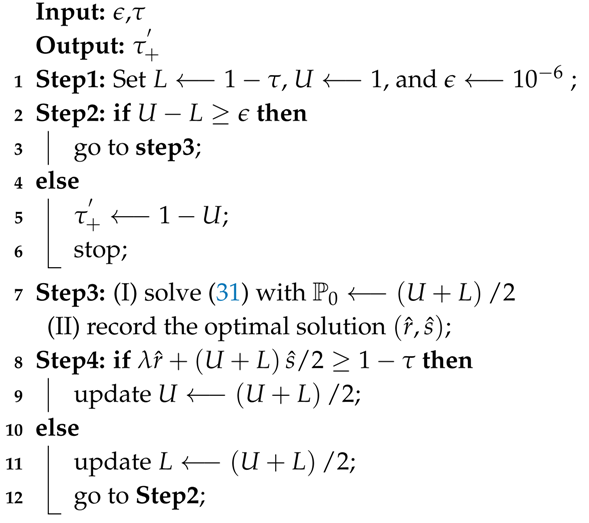
4.2. Sample Average Approximation (SAA)

Due to the intractability of JCC programs, we use the sample approximation in which the distribution of the random $\xi$ vector is replaced with the empirical distribution obtained from the historical data. In the SAA method, an approximation problem, which is based on an independent Monte Carlo samples of the uncertainty vector, is solved. To simplify the presentation, we replace the constraints set $T\left({\mathit{Cap}}^{\mathrm{g}},\xi \right)$ with a real-valued function G as follows:

$$G\left({\mathit{Cap}}^{\mathrm{g}},\xi \right):=\max \left\{T\left({\mathit{Cap}}^{\mathrm{g}},\xi \right)\right\}$$

(32)

Thus, the JCC HC problem can be represented as:

$$\left(P_{{\tau }_{+}^{{}^{\prime }}}\right)z_{{\tau }_{+}^{{}^{\prime }}}^{*}=\min \left\{f\left({\mathit{Cap}}^{\mathrm{g}}\right):{\mathit{Cap}}^{\mathrm{g}}\in {\mathbb{X}}_{{\tau }_{+}^{{}^{\prime }}}\right\}$$

(33)

where,

$${\mathbb{X}}_{{\tau }_{+}^{{}^{\prime }}}=\left\{{\mathit{Cap}}^{\mathrm{g}}\in \mathbb{X}:\mathrm{Pr}\left\{G\left({\mathit{Cap}}^{\mathrm{g}},\xi \right)\le 0\right\}\ge 1-{\tau }_{+}^{{}^{\prime }}\right\}$$

(34)

where, $\mathbb{X}\subset {\mathbb{R}}^n$ represents a deterministic feasible region. Let ${\xi }^1,{\xi }^2,\cdots ,{\xi }^N$ be N independent Monte Carlo samples of the uncertainty vector $\xi$. Then, for $\gamma \in \left[1,0\right)$, the sample approximation problem is defined as follows:

$$\left(P_{\gamma }^N\right){\widehat{z}}_{\gamma }^N=\min \left\{f\left({\mathit{Cap}}^{\mathrm{g}}\right):{\mathit{Cap}}^{\mathrm{g}}\in {\mathbb{X}}_{\gamma }^N\right\}$$

(35)

where,

$${\mathbb{X}}_{\gamma }^N=\left\{{\mathit{Cap}}^{\mathrm{g}}\in \mathbb{X}:\frac{1}{N}\sum _{i=1}^N\mathbb{I}\left(G\left({\mathit{Cap}}^{\mathrm{g}},\xi \right)\le 0\right)\ge 1-\gamma \right\}$$

(36)

where, $\mathbb{I}(·)$ is the indicator function, which takes value one when the argument is true and zero otherwise; $\left(P_{{\tau }_{+}^{{}^{\prime }}}\right)$, and $\left(P_{\gamma }^N\right)$ are referred as the true and SAA problems, respectively. It can be proved that if $\left(P_{{\tau }_{+}^{{}^{\prime }}}\right)$ has an optimal solution, then:

$$\mathrm{Pr}\left\{{\widehat{z}}_{\gamma }^N\le z_{{\tau }_{+}^{{}^{\prime }}}^{*}\right\}\ge \rho \left(\gamma ,{\tau }_{+}^{{}^{\prime }},N\right)$$

(37)

where,

$$\rho \left(\gamma ,{\tau }_{+}^{{}^{\prime }},N\right)=\sum _{i=0}^{\lfloor \gamma N\rfloor }\left(\begin{array}{c}N\\ i\end{array}\right){\left({\tau }_{+}^{{}^{\prime }}\right)}^i{\left(1-{\tau }_{+}^{{}^{\prime }}\right)}^{N-i}$$

(38)

If $\gamma >{\tau }_{+}^{{}^{\prime }}$, then:

$$\mathrm{Pr}\left\{{\widehat{z}}_{\gamma }^N\le z_{{\tau }_{+}^{{}^{\prime }}}^{*}\right\}\ge 1-\exp \left\{-2N{\left(\gamma -{\tau }_{+}^{{}^{\prime }}\right)}^2\right\}$$

(39)

Using M set of N independent samples of $\xi$, the lower bound that is valid with confidence $1-\delta$ can be obtained using Theory 1.

Theory 1.

If $\delta \in \left(0,1\right)$, $\gamma \in \left[0,1\right)$, N, H, and M be positive integer variables such that $H\le M$ and,

$$\sum _{i=0}^{H-1}\left(\begin{array}{c}M\\ i\end{array}\right){\left(\rho \left(\gamma ,{\tau }_{+}^{{}^{\prime }},N\right)\right)}^i{\left(1-\rho \left(\gamma ,{\tau }_{+}^{{}^{\prime }},N\right)\right)}^{N-i}\le \delta$$

(40)

then,

$$\mathrm{Pr}\left\{{\widehat{z}}_{\gamma ,\left[H\right]}^N\le z_{{\tau }_{+}^{{}^{\prime }}}^{*}\right\}\ge 1-\delta$$

(41)

where, ${\widehat{z}}_{\gamma ,\left[H\right]}^N$ is the optimal value of the set H such that ${\widehat{z}}_{\gamma ,\left[1\right]}^N\le \cdots \le {\widehat{z}}_{\gamma ,\left[M\right]}^N$ [31]. Furthermore, it is proven that if $\gamma <{\tau }_{+}^{{}^{\prime }}$, the feasible region of the $\left(P_{\gamma }^N\right)$ will be a subset of the feasible region of the $\left(P_{{\tau }_{+}^{{}^{\prime }}}\right)$. It is also proven that if (1) $\gamma ={\tau }_{+}^{{}^{\prime }}$, (2) the set $\mathbb{X}$ is compact, (3) the function $f\left({\mathit{Cap}}^{\mathrm{g}}\right)$ is continuous, (4) $G\left({\mathit{Cap}}^{\mathrm{g}},\xi \right)$ is a Caratheodory function, and (5) there is an optimal solution $\overline{{\mathit{Cap}}^{\mathrm{g}}}$ of the true problem such that for all $\epsilon >0$ there is ${\mathit{Cap}}^{\mathrm{g}}\in \mathbb{X}$ in $\parallel {\mathit{Cap}}^{\mathrm{g}}-\overline{{\mathit{Cap}}^{\mathrm{g}}}\parallel \le \epsilon$ and $\mathrm{Pr}\left\{G\left({\mathit{Cap}}^{\mathrm{g}},\xi \right)\le 0\right\}\ge 1-{\tau }_{+}^{{}^{\prime }}$, then, ${\widehat{z}}_{\gamma }^N⟶z_{{\tau }_{+}^{{}^{\prime }}}^{*}$ [32]. The sample approximation problem (35) is reformulated as a mix-integer problem as follows:

$$\begin{array}{c}\underset{Ca{p}_j^{\mathrm{g}}}{\mathrm{minimize}}\sum _{j\in \mathcal{DG}}-Ca{p}_j^{\mathrm{g}}\hfill \\ \mathrm{s}.\mathrm{t}.\hfill \\ G\left({\mathit{Cap}}^{\mathrm{g}},{\xi }^{\mathbf{j}}\right)\le M_j{Z}_j\forall j\in \left\{1,2,\cdots ,N\right\}\hfill \\ \sum _{j=1}^N{Z}_j\le \gamma N\hfill \\ Z_j\in \left\{0,1\right\}\forall j\in \left\{1,2,\cdots ,N\right\}\hfill \\ {\mathit{Cap}}^{\mathrm{g}}\in \mathbb{X}\hfill \end{array}$$

(42)

where, $Z_j$ is a binary variable and $M_j$ is a large positive number.

5. Numerical Results

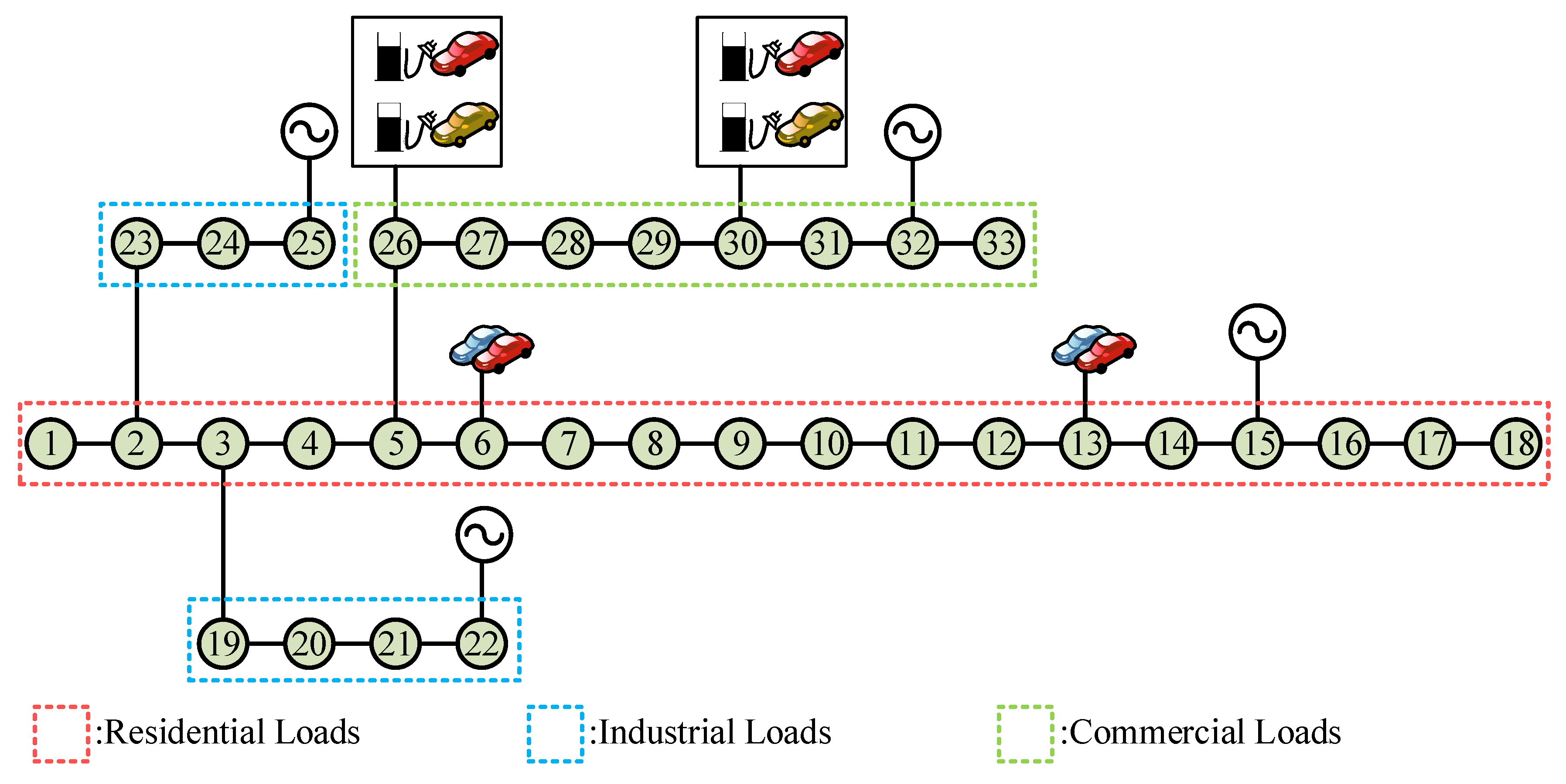
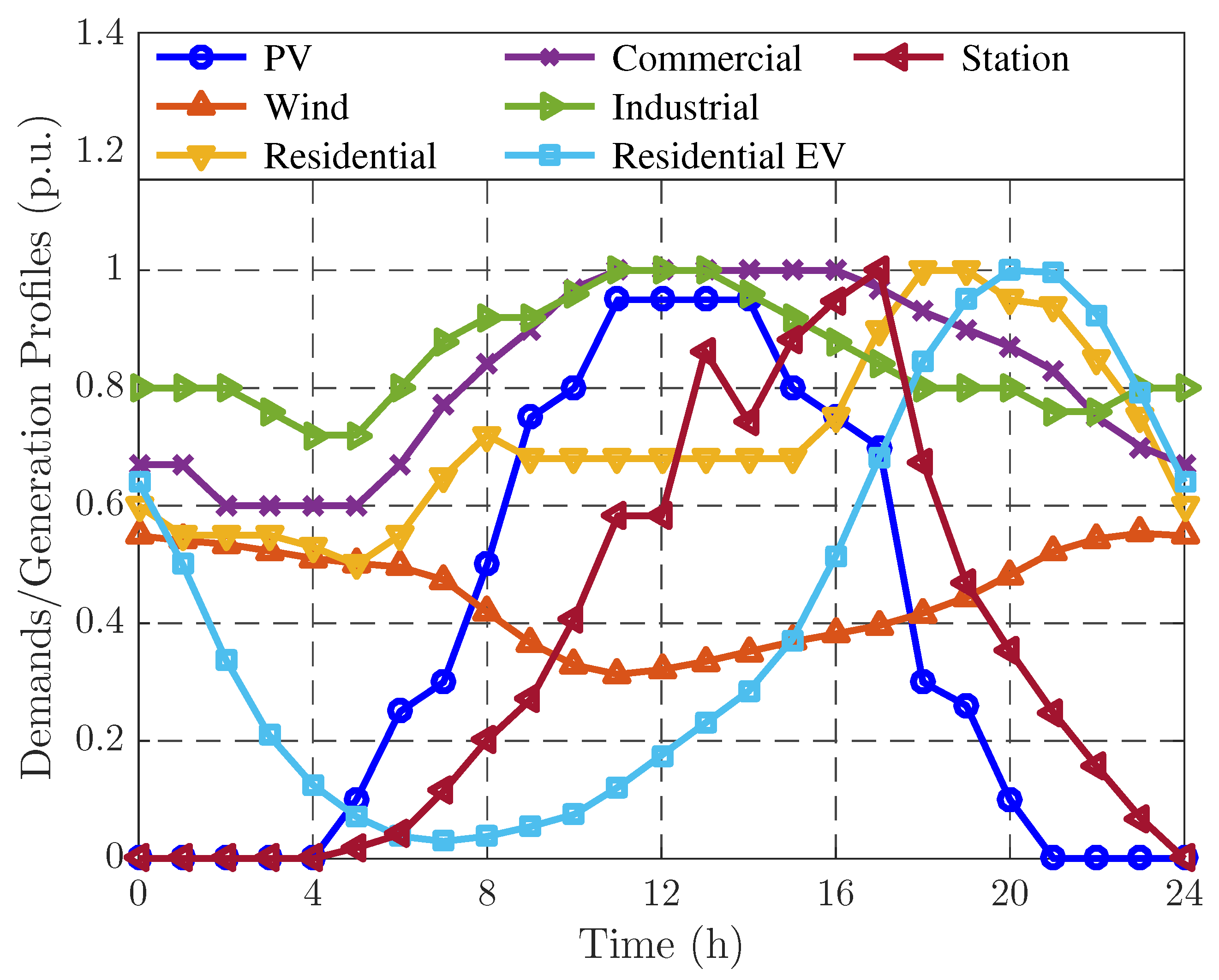
In this section, simulations are carried out to assess the performance of the proposed methodology. Firstly, the modified IEEE 33-bus network is presented in Section 5.1. Then, the efficacy of the proposed method is evaluated in Section 5.2.

5.1. Test System

The performance of the proposed method is evaluated on the modified IEEE 33-bus system, shown in Figure 2. The bus 1 is connected to the 33 kV grid using a Dy transformer with 8.5% reactance. The SCL and the rated SCL at the 33kV side are 200 MVA and 250 MVA, respectively. The system nominal voltage is 12.66 kV.

There are four candidate sites for DGs, i.e., $\mathcal{DG}=\left\{15,22,25,32\right\}$. There are two charging stations at buses 26 and 30. Additionally, the charging demand of EVs in the residential area is aggregated at buses 6 and 13. The detail description of the test system is presented in [33]. To have a real situation, three load models (i.e., industrial, commercial, and residential) are considered, as shown in Figure 2. The PV and wind generation profiles, the aggregated EVs charging demand in residential area, the EV charging station demand curve and the load profiles are provided in Figure 3. The PV output profile and the residential, commercial, and industrial load profiles are general profiles that are derived from [13]. The aggregated EVs demand profile is derived from [34,35], which are based on the National Household Travel Survey (NHTS). As for the demand of charging stations, the obtained profile using the NHTS data provided in [29] is used. Since the NHTS data presents the driving behavior of American public, the wind generation profile is derived from the data provided for the continental United States in [36]. The presented curves in Figure 3 are normalized multipliers. Please note that basic values of DGs and loads are the capacity of DGs and the nominal loads, respectively. The basic value for charging stations’ demand is 224 kW and for aggregated demand of residential EV is 285 kW.

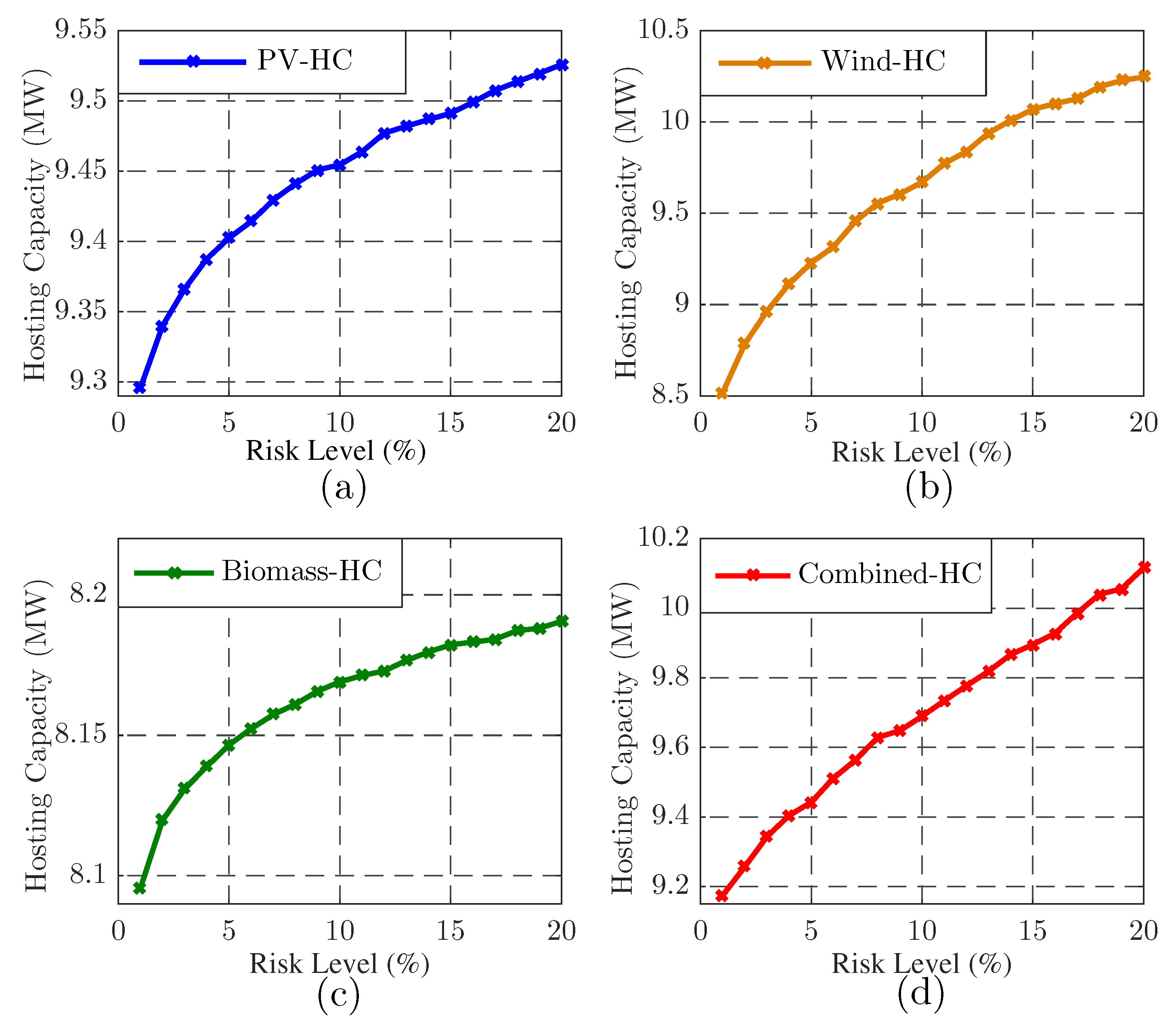
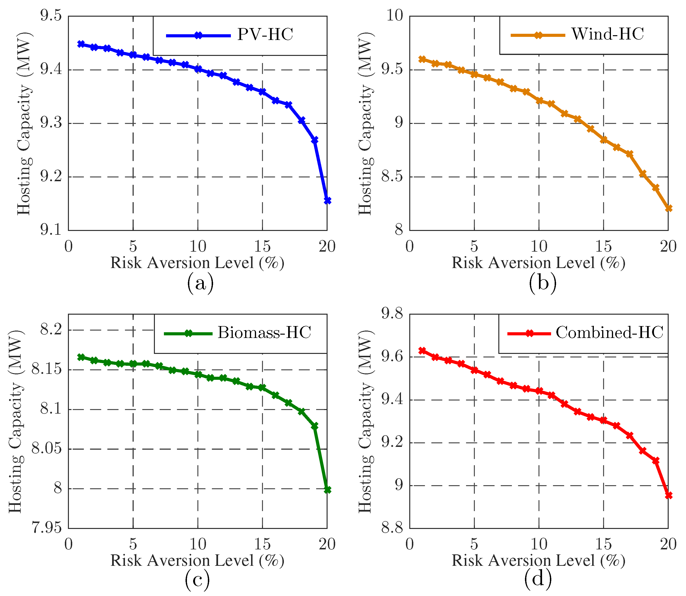
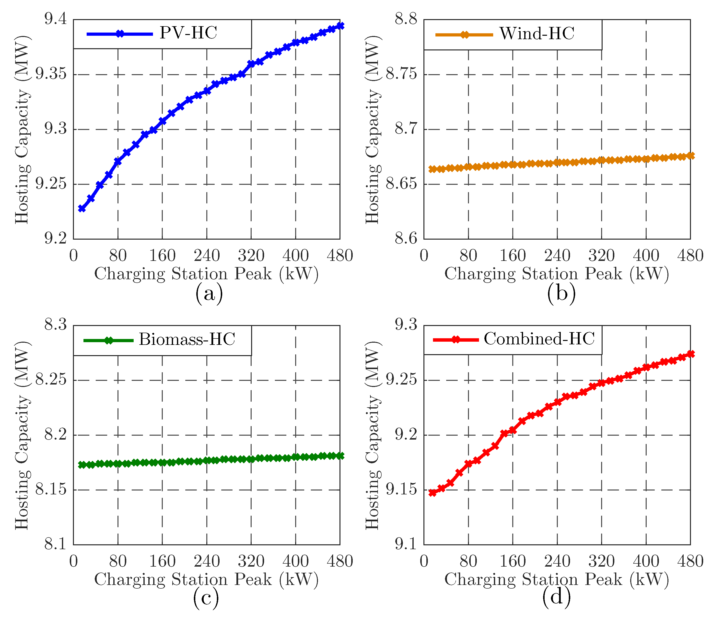
5.2. Simulation Results on the Modified IEEE 33-Bus System

The proposed DRO-based method is examined on the IEEE 33-bus system for the four cases as follows:

• PV-HC: All DGs are PV systems.
• Wind-HC: All DGs are wind generators.
• Biomass-HC: All DGs are biomass generators.
• Combined-HC: The DGs at buses 15 and 32 are PV units, and the DGs at buses 22 and 25 are wind and biomass generators, respectively.

Figure 4 shows the estimated HC of different generation technologies for different risk levels. Observe that the HC grows by increasing the risk level, which indicates that looser security requirement leads to a higher HC. Furthermore, as can be seen in Figure 4, the HC curve slope depends on the DG technology. For instance, accepting 20% security risk, increases the HC by 2.48%, 20.3% and 1.17% for PV, wind, and biomass technologies, respectively. This implies that accepting a higher risk to increase the HC of the system is not a good idea if the DGs technologies are PV and biomass.

An important factor that affects the estimated HC of the system is the existence of the historical data. Intuitively, as the sample size of historical data increases, the empirical distribution becomes closer to the actual distribution. Thus, the conservativeness of the HC estimation decreases. In DRO-based method, $\psi$ is the parameter to present the value of data. The higher the number of samples, the more accurate the empirical distribution, the smaller the risk-aversion level, $\psi$, and the smaller the confidence set, ${\mathcal{D}}_{\varphi }$. Figure 5 demonstrates the effect of risk-aversion level (hence historical data) on the HC for different technologies. As it can be seen in Figure 5, the shortage of historical data increases the conservativeness of the HC estimation. For instance, the shortage of data decreases the estimated HC for PV, wind, and biomass technologies by 3.09%, 14.52% and 2.06%, respectively. Observe that the value of data in the test system for wind technology is much higher than that of PV or biomass technologies. Furthermore, as the slope of HC curves for small values of risk-aversion level (i.e., $\psi \in [0\%,5\%]$) is small, increasing the size of historical data to get a more accurate empirical distribution does not have a tangible effect on the estimated HC. As shown in Figure 5, 5% error in empirical distributions only decreases the HC by 0.21%, 1.41%, and 0.11% for PV, wind, and biomass technologies, respectively.

A prospective technology that may affect the HC of a system is EVs. Figure 6 indicates the effect of EVs’ aggregated demand on the HC. Observe that increasing the peak value of EVs’ aggregated demand to 640 kW can only increase the HC of the system by 0.29%, 0.25%, and 0.13% for PV, wind and biomass technologies, respectively. Thus, the aggregated impact of EV loads on the HC of the system is not tangible. This is because the HC reaches its maximum value during time period $t=11$ for PV, $t=5$ for wind, $t=5$ for biomass and $t=9$ for combined generation. We will call these periods as the critical time periods. During critical time periods, the normalized aggregated demand of residential EVs is below 10%, which means that increasing the EVs cannot effectively increase the load. To demonstrate that the concluded result does not depend on the aggregation points of EVs, the sensitivity of the HC to the location of aggregated EVs demand is also presented using error bars in Figure 6.

Observe that changing the location of aggregated demand of residential EVs deviates the obtained HC by 0.068%, 0.072%, and 0.032% for PV, wind, and biomass technologies, respectively. In other words, irrespective of locations that demands of residential EVs are aggregated, increasing the peak value of aggregated EVs demand does not increase the HC, effectively.

Finally, the effect of charging stations’ demands on the HC is assessed. To do so, the peak value of charging stations’ demands is varied from 0 kW to 480 kW, as shown in Figure 7. Observe that increasing the demand of charging stations can linearly increase the HC of the system. However, the rate of increase in the HC depends on the generation technology. Increasing the peak value of charging stations’ demands from 0 to 480 kW grows the HC by 1.81%, 0.15%, and 0.1% for PV, wind, and biomass technologies, respectively. This is because the critical time period depends on the DGs technologies. The charging station demand profile at critical time period for PV, wind, biomass, and combined generations are 58.26%, 1.83%, 1.83%, and 27.06%, respectively. Since the demand profile of charging stations during the critical time period of PV generation is higher than that of other technologies, the charging stations’ demands have a higher effect on the HC of the system for PV generation.

6. Conclusions

In this paper, a DRO-based method is proposed to assess the HC of distribution networks. In the proposed method, the empirical distributions of uncertain variables are used to define a confidence set. The more accurate the empirical distribution is, the smaller the confidence set and the less conservative the obtained result would be. The effectiveness of the proposed method was examined on the modified IEEE 33-bus system and the effects of risk level and size of historical data on the HC of the system were assessed. It was demonstrated that the proposed method yields in a less conservative solution by increasing the risk level. However, the increase in the HC by accepting a higher risk level depends on the DG technology. For instance, accepting 20% risk level can increase the HC of the system by 2.48%, 20.3% and 1.17% for PV, wind and biomass technologies, respectively. Thus, accepting a higher risk level to increase the HC of the test system may not be a good idea if the DGs technologies are PV and biomass. As for the historical data, it was observed that shortage of data can exponentially increase the conservativeness of the estimated HC. For instance, the shortage of historical data decreases the estimated HC for wind technology up to 14.52%.

The proposed method is also used to assess the effects of the aggregated residential EVs and charging stations’ demand on the HC for different DG technologies. Following are the conclusions derived from the simulation results:

• Although aggregated demand of residential EVs increases the peak load of the distribution system, it does not affect the HC significantly. This is because the HC of the system reaches its maximum value during the time periods that the aggregated demand of EVs is below 10% of its peak value.

• The effect of charging stations’ demand on the HC depends on the DG technology. If DGs are PV units, increasing the charging stations’ demand to its maximum increases the HC up to 1.81%. Nevertheless, it cannot effectively increase the HC of the system if DGs are wind and biomass generators.

A future extension would be considering the uncertainty associated with the location of DGs. To do so, the developed mathematical model should be integrated in a Monte Carlo-based framework.

References

1. Akbari, M.A.; Aghaei, J.; Barani, M.; Savaghebi, M.; Shafie-Khah, M.; Guerrero, J.M.; Catalão, J.P. New metrics for evaluating technical benefits and risks of DGs increasing penetration. IEEE Trans. Smart Grid 2017, 8, 2890–2902. [Google Scholar] [CrossRef]
2. Wang, S.; Chen, S.; Ge, L.; Wu, L. Distributed generation hosting capacity evaluation for distribution systems considering the robust optimal operation of OLTC and SVC. IEEE Trans. Sustain. Energy 2016, 7, 1111–1123. [Google Scholar] [CrossRef]
3. Vovos, P.N.; Harrison, G.P.; Wallace, A.R.; Bialek, J.W. Optimal power flow as a tool for fault level-constrained network capacity analysis. IEEE Trans. Power Syst. 2005, 20, 734–741. [Google Scholar] [CrossRef] [Green Version]
4. Dent, C.J.; Ochoa, L.F.; Harrison, G.P. Network distributed generation capacity analysis using OPF with voltage step constraints. IEEE Trans. Power Syst. 2010, 25, 296–304. [Google Scholar] [CrossRef]
5. Abad, M.S.S.; Verbič, G.; Chapman, A.; Ma, J. A linear method for determining the hosting capacity of radial distribution systems. In Proceedings of the Universities Power Engineering Conference (AUPEC), Melbourne, Australasian, 19–22 November 2017; pp. 1–6. [Google Scholar]
6. Mahmud, M.A.; Hossain, M.J.; Pota, H.R. Voltage variation on distribution networks with distributed generation: Worst case scenario. IEEE Syst. J. 2014, 8, 1096–1103. [Google Scholar] [CrossRef]
7. Koutroumpezis, G.N.; Safigianni, A.S. Optimum allocation of the maximum possible distributed generation penetration in a distribution network. Electr. Power Syst. Res. 2010, 80, 1421–1427. [Google Scholar] [CrossRef]
8. Ochoa, L.F.; Padilha-Feltrin, A.; Harrison, G.P. Time-series-based maximization of distributed wind power generation integration. IEEE Trans. Energy Convers. 2008, 23, 968–974. [Google Scholar] [CrossRef]
9. Ding, F.; Mather, B. On Distributed PV Hosting Capacity Estimation, Sensitivity Study, and Improvement. IEEE Trans. Sustain. Energy 2017, 8, 1010–1020. [Google Scholar] [CrossRef]
10. Arshad, A.; Lindner, M.; Lehtonen, M. An Analysis of Photo-Voltaic Hosting Capacity in Finnish Low Voltage Distribution Networks. Energies 2017, 10, 1702. [Google Scholar] [CrossRef]
11. Abad, M.S.S.; Ma, J.; Zhang, D.; Ahmadyar, A.S.; Marzooghi, H. Probabilistic Assessment of Hosting Capacity in Radial Distribution Systems. IEEE Trans. Sustain. Energy 2018. [Google Scholar] [CrossRef]
12. Navarro-Espinosa, A.; Ochoa, L.F. Probabilistic impact assessment of low carbon technologies in LV distribution systems. IEEE Trans. Power Syst. 2016, 31, 2192–2203. [Google Scholar] [CrossRef]
13. Chen, X.; Wu, W.; Zhang, B. Robust Capacity Assessment of Distributed Generation in Unbalanced Distribution Networks Incorporating ANM Techniques. IEEE Trans. Sustain. Energy 2018, 9, 651–663. [Google Scholar] [CrossRef] [Green Version]
14. Santos, S.F.; Fitiwi, D.Z.; Shafie-Khah, M.; Bizuayehu, A.W.; Cabrita, C.M.; Catalão, J.P. New multistage and stochastic mathematical model for maximizing res hosting capacity—part I: problem formulation. IEEE Trans. Sustain. Energy 2017, 8, 304–319. [Google Scholar] [CrossRef]
15. Chen, X.; Wu, W.; Zhang, B.; Lin, C. Data-driven dg capacity assessment method for active distribution networks. IEEE Trans. Power Syst. 2017, 32, 3946–3957. [Google Scholar] [CrossRef]
16. Abad, M.S.S.; Ma, J.; Zhang, D.; Ahmadyar, A.S.; Marzooghi, H. Sensitivity of Hosting Capacity to Data Resolution and Uncertainty Modeling. In Proceedings of the 2018 Australasian Universities Power Engineering Conference (AUPEC), Auckland, New Zealand, 19–22 November 2017; pp. 1–6. [Google Scholar]
17. Xiong, P.; Jirutitijaroen, P.; Singh, C. A distributionally robust optimization model for unit commitment considering uncertain wind power generation. IEEE Trans. Power Syst. 2017, 32, 39–49. [Google Scholar] [CrossRef]
18. Wang, Z.; Bian, Q.; Xin, H.; Gan, D. A distributionally robust co-ordinated reserve scheduling model considering CVaR-based wind power reserve requirements. IEEE Trans. Sustain. Energy 2016, 7, 625–636. [Google Scholar] [CrossRef]
19. Abad, M.S.S.; Ma, J.; Han, X. Distribution systems hosting capacity assessment: Relaxation and linearization. In Smart Power Distribution Systems, Control, Communication, and Optimization; Academic Press: Cambridge, MA, USA, 2018. [Google Scholar]
20. Boutsika, T.N.; Papathanassiou, S.A. Short-circuit calculations in networks with distributed generation. Electr. Power Syst. Res. 2008, 78, 1181–1191. [Google Scholar] [CrossRef]
21. Keane, A.; O’Malley, M. Optimal allocation of embedded generation on distribution networks. IEEE Trans. Power Syst. 2005, 20, 1640–1646. [Google Scholar] [CrossRef]
22. Baran, M.E.; Hooshyar, H.; Shen, Z.; Huang, A. Accommodating high PV penetration on distribution feeders. IEEE Trans. Smart Grid 2012, 3, 1039–1046. [Google Scholar] [CrossRef]
23. Xu, Y.; Dong, Z.Y.; Zhang, R.; Hill, D.J. Multi-timescale coordinated voltage/var control of high renewable-penetrated distribution systems. IEEE Trans. Power Syst. 2017, 32, 4398–4408. [Google Scholar] [CrossRef]
24. Fabbri, A.; Roman, T.G.S.; Abbad, J.R.; Quezada, V.M. Assessment of the cost associated with wind generation prediction errors in a liberalized electricity market. IEEE Trans. Power Syst. 2005, 20, 1440–1446. [Google Scholar] [CrossRef]
25. Atwa, Y.M.; El-Saadany, E.F.; Salama, M.M.A.; Seethapathy, R. Optimal renewable resources mix for distribution system energy loss minimization. IEEE Trans. Power Syst. 2010, 25, 360–370. [Google Scholar] [CrossRef]
26. Wang, Z.; Wang, J.; Chen, B.; Begovic, M.M.; He, Y. MPC-based voltage/var optimization for distribution circuits with distributed generators and exponential load models. IEEE Trans. Smart Grid 2014, 5, 2412–2420. [Google Scholar] [CrossRef]
27. Li, G.; Zhang, X.P. Modeling of plug-in hybrid electric vehicle charging demand in probabilistic power flow calculations. IEEE Trans. Smart Grid 2012, 3, 492–499. [Google Scholar] [CrossRef]
28. Tehrani, N.H.; Wang, P. Probabilistic estimation of plug-in electric vehicles charging load profile. Electr. Power Syst. Res. 2015, 124, 133–143. [Google Scholar] [CrossRef]
29. Alharbi, W.; Bhattacharya, K. Electric vehicle charging facility as a smart energy microhub. IEEE Trans. Sustain. Energy 2017, 8, 616–628. [Google Scholar] [CrossRef]
30. Jiang, R.; Guan, Y. Data-driven chance constrained stochastic program. Math. Program. 2016, 158, 291–327. [Google Scholar] [CrossRef]
31. Luedtke, J.; Ahmed, S. A sample approximation approach for optimization with probabilistic constraints. SIAM J. Optim. 2008, 19, 674–699. [Google Scholar] [CrossRef]
32. Pagnoncelli, B.K.; Ahmed, S.; Shapiro, A. Sample average approximation method for chance constrained programming: theory and applications. J. Optim. Theory Appl. 2009, 142, 399–416. [Google Scholar] [CrossRef]
33. Gharigh, M.K.; Abad, M.S.S.; Nokhbehzaeem, J.; Safdarian, A. Optimal sizing of distributed energy storage in distribution systems. In Proceedings of the Smart Grid Conference (SGC), Tehran, Iran, 22–23 December 2015; pp. 60–65. [Google Scholar]
34. Tan, J.; Wang, L. Integration of plug-in hybrid electric vehicles into residential distribution grid based on two-layer intelligent optimization. IEEE Trans. Smart Grid 2014, 5, 1774–1784. [Google Scholar] [CrossRef]
35. Darabi, Z.; Ferdowsi, M. Aggregated impact of plug-in hybrid electric vehicles on electricity demand profile. IEEE Trans. Sustain. Energy 2011, 2, 501–508. [Google Scholar] [CrossRef]
36. Draxl, C.; Clifton, A.; Hodge, B.M.; McCaa, J. The wind integration national dataset (WIND) Toolkit. Appl. Energy 2015, 151, 355–366. [Google Scholar] [CrossRef]
Figure 1. The HC calculation framework.
Energies 11 02981 g001
Figure 2. The modified IEEE 33-bus distribution system.
Energies 11 02981 g002
Figure 3. The daily PV, wind, aggregated EVs, charging stations and load normalized profiles.
Energies 11 02981 g003
Figure 4. The HC obtained via the proposed DRO-HC method with different risk levels for different technologies including: (a) PV; (b) wind; (c) biomass; and (d) combination of PV, wind and biomass.
Energies 11 02981 g004
Figure 5. The value of data for the HC obtained via the proposed DRO-HC method with τ = 10 % for different technologies including: (a) PV; (b) wind; (c) biomass; and (d) combination of PV, wind and biomass.
Energies 11 02981 g005
Figure 6. The effect of aggregate demand of residential EVs on the HC obtained via the proposed DRO-HC method with τ = 1 % for different technologies including: (a) PV; (b) wind; (c) biomass; and (d) combination of PV, wind and biomass.
Energies 11 02981 g006
Figure 7. The effect of charging stations’ demands on the HC obtained via the proposed DRO-HC method with τ = 1 % for different technologies including: (a) PV; (b) wind; (c) biomass; and (d) combination of PV, wind and biomass.
Energies 11 02981 g007