An Effective Ground Fault Location Scheme Using Unsynchronized Data for Multi-Terminal Lines

Abstract

Traveling-wave-based methods perform poorly for the fault location of multi-terminal lines as a result of the limitation introduced by being a highly branched structure. The requirement for multi-terminal time synchronization is also a drawback and needs to be improved. In this paper, an effective fault location method for use on multi-terminal lines is proposed, and it does not require the data from each terminal to be synchronized. The method is based on the arrival time differences in the ground and aerial mode waves detected at each terminal. First, fault section identification rules for a three-terminal line are proposed. Then, a multi-terminal topological structure in this paper will be deemed as one consisting of multiple three-terminal lines. Thus, a whole scheme to identify any fault section in a multi-terminal line is presented. Consequently, the fault distance is calculated using the fault distance ratios in the corresponding fault section. The advantage of the proposed scheme is that complete coverage of multi-terminal lines fault location can still be achieved once some synchronized devices are out of operation. To evaluate the performance of the proposed method, many fault cases under different conditions are implemented. The simulation results show that the proposed method can identify the fault section correctly and locate the fault more accurately and reliably than existing methods.

1. Introduction

Ground faults are the most frequent occurrence in the power system and may cause customer service interruptions [1]. The accurate location of faults is important for faster system restoration and reducing economic loss. Therefore, a number of fault location techniques have been actively developed. Fault location methods have been widely used for achieving satisfactory results in two-terminal transmission lines [2,3]. However, the fault location technique of multi-terminal lines is not as simple as that of two-terminal lines. Additional problems may be caused by a complex network topology and multi-terminal synchronous measurement, which restrict the research of fault location. The accurate location of faults in multi-terminal lines is necessary to solve the issue in a better manner.

Various methods used for fault location have been reported in the literature, and are usually divided into three categories: impedance-based methods [4], traveling-wave-based methods [5,6], and artificial intelligence-based methods [7,8]. Among these methods, the fault location methods based on steady-state components (the impedance-based methods) have become promising with the applications of phasor measurement units (PMUs) [9,10,11]. A synchronized PMU-based fault location technique is presented for hybrid multi-terminal nonhomogeneous transmission lines in the literature [11], which has the advantage of being insusceptible to source impedance. However, global positioning system (GPS)-aided PMUs may be not widely adopted in practice because of economic considerations. In the works of [12,13], unsynchronized measurements in impedance-based methods have also been studied and used for the fault location of three-terminal and multi-terminal lines. However, a series of errors caused by the line parameters, shunt capacitance, fault resistances, or current transformer saturation influences most impedance-based methods [14]. The traveling-wave fault location methods based on transient-state analysis are more stable with respect to the above factors. It is well known that the traveling-wave-based methods present better performance because fault-induced transient detection depends mainly on the sampling rates of the data acquisition system [15]. In the literature [16,17,18,19,20,21,22,23], several transient fault detection methods and their performances are introduced; in the work of [17], the linear regression coefficients indices (LRCIs) of current signals are computed to accomplish the fault detection and classification process. A sweep frequency response analysis (SFRA) technique was used to detect the transformer winding faults [18]. In the work of [19], features extraction using qualitative trend analysis (QTA) is proposed for multiple faults because they possess similar patterns compared with single faults, and the features extraction method of single fault is limited. The authors of [20] recognize armature current and diagnose the fault of a DC generator with the use of fast Fourier transform (FFT), the method of selection of amplitudes of frequencies (MSAF-1), and linear discriminant analysis (LDA). FFT can provide good frequency information, but time information is lost. Wavelet transform (WT) is a powerful tool and has been widely used because of its good time-frequency characteristics. The stationary wavelet transform (SWT) is applied for fault detection [21] and discrete wavelet transform (DWT) is frequently used for the detection of arrival times in the traveling-wave-based method [22,23].

The artificial intelligence (AI)-based methods have shown advantages regarding fault classification and fault section identification [24,25,26]. In the work of [26], a self-learning fault classifier based on modified fuzzy Q learning is proposed for a transmission line. Compared with conventional AI techniques for fault classification—artificial neural network (ANN) and support vector machine (SVM)—this classifier can also achieve a high accuracy. However, in aiming to estimate accurate fault points, these AI-based methods are usually combined with other fault location methods. Furthermore, most methods require the performance of fault classification and location independently and sequentially. However, in another paper [27], an integrated framework is proposed by using the summation-Gaussian extreme learning machine, which is fully self-learning and does not require standalone feature extraction. The disadvantages of these methods are that they need accurate and time-consuming training on all possible fault conditions and network topologies.

The traveling-wave-based methods can be further divided into two types: one-terminal and two-terminal fault location methods. The two-terminal methods are widely used in many kinds of line structures. Locating a fault for multi-terminal lines generally first requires the identification of a faulty line section. In the work of [28], the two-terminal method with SVM classifiers is presented for a three-terminal line. However, selecting proper SVM parameters and obtaining the learning datasets requires a large amount of time. In a further paper [29], the matrix of the time difference of arrival is utilized for faulty line identification of Y type multi-terminal lines (all branches have a common joint point). In the work of [30], the faulty section identification rules and the fault location method are proposed based on current traveling waves for multi-terminal lines with many tap nodes. In another paper [31], three arrival times of traveling waves are first applied to identify a three-terminal fault section from multi-terminal lines. In a further paper [32], a multi-terminal technique to locate faults directly on branched networks has also been described. However, in the above methods, the arrival times detected from all terminals must be synchronized using GPS, and the loss of a common time reference will cause errors. Moreover, errors in calculated traveling-wave velocity also influence accuracy of the fault location methods. However, very little research to solve these issues on traveling-wave-based fault location for multi-terminal lines has been conducted. A traveling-wave-based fault location using unsynchronized data for a two-terminal line has been proposed [33], but an additional communication system is required to exchange data between the two terminals.

In fact, one-terminal methods do not require time synchronization, but the reflected wave from the fault point is very difficult to distinguish in multi-terminal lines. For the ground fault, the one-terminal methods based on ground and aerial mode traveling waves have been reported [34,35,36]. The mode propagation time difference of the initial wave is used to eliminate the need for the reflected wave; although, ground and aerial mode velocities are also required in the fault location formula. The asynchronous fault location technique is implemented considering the attenuation characteristic of ground mode velocity [35]. A two-terminal method based on mode time difference is presented in the literature [36], which does not require synchronized time. However, all of these methods are used to estimate the fault point for two-terminal lines. The method based on the time difference of mode traveling waves is not yet used for multi-terminal complex topologies.

Aiming to locate a fault in multi-terminal lines, the most important step is to identify a certain fault section. The main contribution of this paper is to propose a new fault section identification and fault location method for multi-terminal lines based on the time difference of mode traveling waves. The proposed method cannot be restricted by the multi-terminal time synchronization. The proposed fault section identification and fault location method are presented in the rest of this paper. The fault cases under different conditions are simulated. Finally, the evaluation and comparison are provided to demonstrate the effectiveness of the proposed method.

2. Proposed Fault Location Method

In this paper, a multi-terminal traveling wave fault location network is built and is shown in Figure 1. When a fault occurs, the waveforms of the fault-induced traveling waves are recorded at substations. The fault information can be sent to control center via wireless transmission or optical fiber transmission. The wireless transmission generally includes GPRS (General Packet Radio Service), 4G and WIFI. The optical fiber transmission requires to use the OPGW (Optical Fiber Composite Overhead Ground Wire) and the SPI (Serial Peripheral Interface). The arrival time detection of the initial wave and fault location algorithm are implemented in cloud platform and the network status is monitored by computers. The core idea of this paper is the research of fault section identification and fault location algorithm. The proposed method is based on the one-terminal fault location method using the time difference of modes. Figure 2 shows a time–space diagram for a two-terminal line monitored at terminals L and R. The algorithm uses two functional modules: fault detection module and fault location module. v₀ and v₁ are the ground and aerial mode propagation velocities, respectively. t_L(0), t_L(1), t_R(0), and t_R(1) are the arrival times of the first ground and aerial mode waves at terminals L and R. When a fault occurs, the fault distance is obtained as follows:

$$d_{\mathrm{F}X}=\Delta t_X{v}_0{v}_1/(v_1-v_0)$$

(1)

where Δt_X = t_X(0) − t_X(1), and X is called terminal index, including L and R in Figure 2. The accurate detection of arrival times of transient traveling waves is important for fault location. Current transformers (CTs) are typical devices that detect current traveling waves in many studies. A CT must measure currents in each line of substation, which complicates the fault location system. In addition, the current traveling waves are susceptible to disturbances, which causes detection errors. The detection of voltage traveling waves with good sensitivity has been used in transmission lines [37,38]. The voltage magnitude of traveling waves increases at the instant of fault incidence, which is good for the detection of voltage traveling waves. Although the coupling capacitor voltage transformers (CCVT) have limited bandwidths, the proposed method in the literature [39] is available for the correction of the CCVT transient response. The CCVT is also indicated have a good performance for transient voltage measurement [40]. In this paper, the voltage traveling waves are measured, and the ground and aerial mode quantities are computed through the Karrenbauer transformation. The Karrenbauer transformation, shown in Equation (2), is applied for transforming the coupled voltage phase components to independent modal components. u_a, u_b, and u_c denote the phase voltages; u₁ and u₂ are the aerial-mode voltages; and u₀ is the ground-mode voltage.

$$\left[\begin{array}{c}{u}_0\\ u_1\\ u_2\end{array}\right] =\frac{1}{3}\left[\begin{array}{ccc}1& 1& 1\\ 1& -1& 0\\ 1& 0& -1\end{array}\right]\left[\begin{array}{c}{u}_a\\ u_b\\ u_c\end{array}\right]$$

(2)

A discrete wavelet transformation (DWT) is applied to decompose the mode voltage at the terminals. The wavelet decomposition process for signal is shown in Figure 3, and f_s is the sampling frequency. The first arrival times of traveling waves are obtained by observing wavelet transformation coefficient squared (WTC²_S).

The proposed fault location procedure for multi-terminal lines starts with the above fault-induced voltage transient detection at each terminal. The core ideas of the proposed method are to identify a fault section and locate a fault point accurately, which are described in the following sections.

2.1. Rules for Fault Section Identification in Three-Terminal Lines

Consider the three-terminal topology shown in Figure 4, where L, R, and B1 are terminal indices, and T is a tap node. Line L–R is defined as a main line, and line sections T–L, T–R, and T–B1 are defined as branch lines. l is the line length; for example, l_TB1 is the line length between tap node T and terminal B1. d represents the fault distance. When a fault occurs, the arrival times of the initial traveling waves are detected at terminals L, R, and B1. According to Equation (1), the fault distance from fault point F to all these terminals are calculated as follows:

$$d_{\mathrm{FL}}=\Delta t_{\mathrm{L}}{v}_0{v}_1/(v_1-v_0)$$

(3)

$$d_{\mathrm{FR}}=\Delta t_{\mathrm{R}}{v}_0{v}_1/(v_1-v_0)$$

(4)

$$d_{\mathrm{FB}1}=\Delta t_{\mathrm{B}1}{v}_0{v}_1/(v_1-v_0)$$

(5)

among them, Δt_L = t_L(0) − t_L(1), Δt_R = t_R(0) − t_R(1), and Δt_B1 = t_B1(0) − t_B1(1). Suppose v₀ and v₁ are constant in lines, a series of fault distance ratios are further calculated as follows:

$$r_{\mathrm{LR}}=d_{\mathrm{FL}}/d_{\mathrm{FR}}=\Delta t_{\mathrm{L}}/\Delta t_{\mathrm{R}}$$

(6)

$$r_{\mathrm{LB}1}=d_{\mathrm{FL}}/d_{\mathrm{FB}1}=\Delta t_{\mathrm{L}}/\Delta t_{\mathrm{B}1}$$

(7)

$$r_{\mathrm{RB}1}=d_{\mathrm{FR}}/d_{\mathrm{FB}1}=\Delta t_{\mathrm{R}}/\Delta t_{\mathrm{B}1}$$

(8)

where r_LR, r_LB1, and r_RB1 are fault distance ratios. It is shown that Equations (6)–(8) only contain the arrival times of ground and aerial mode traveling waves, and the velocity terms are eliminated in this way. Furthermore, the synchronized time is dispensable because the time differences are measured separately at terminals. Then, a fault distance ratio matrix (FDRM) M with three rows and three columns can be built for the three-terminal line in the following form:

$$M=\begin{array}{c}\begin{array}{ccc}\mathrm{L}& \mathrm{R}& \mathrm{B}1\end{array}\\ \begin{array}{c}\mathrm{L}\\ \mathrm{R}\\ \mathrm{B}1\end{array}\left[\begin{array}{ccc}1& r_{\mathrm{LR}}& r_{\mathrm{LB}1}\\ 1/r_{\mathrm{LR}}& 1& r_{\mathrm{RB}1}\\ 1/r_{\mathrm{LB}1}& 1/r_{\mathrm{RB}1}& 1\end{array}\right]\end{array}$$

(9)

In addition, a branch distance ratio matrix (BDRM) for the three-terminal line is shown with P as follows:

$$P=\begin{array}{c}\begin{array}{ccc}\mathrm{L}& \mathrm{R}& \mathrm{B}1\end{array}\\ \begin{array}{c}\mathrm{L}\\ \mathrm{R}\\ \mathrm{B}1\end{array}\left[\begin{array}{ccc}1& l_{\mathrm{TL}}/l_{\mathrm{TR}}& l_{\mathrm{TL}}/l_{\mathrm{TB}1}\\ l_{\mathrm{TR}}/l_{\mathrm{TL}}& 1& l_{\mathrm{TR}}/l_{\mathrm{TB}1}\\ l_{\mathrm{TB}1}/l_{\mathrm{TL}}& l_{\mathrm{TB}1}/l_{\mathrm{TR}}& 1\end{array}\right]\end{array}$$

(10)

where elements in the matrix are line length ratios of branch lines, which are known as priori values in the network. To identify the fault section, comparing matrix M and P, the distance ratio difference matrix (DRDM) ∆ is defined as follows:

$$\Delta =M-P$$

(11)

In matrix ∆, the element in the ith row and jth column is recorded as ∆_ij. Each element is compared with the value 0. In different fault sections (fault in T–L, T–R, and T–B1), different results are recorded as ∆_T–L, ∆_T–R, and ∆_T–B1, separately, as follows:

$${\Delta }_{\mathrm{T}–\mathrm{L}}=\begin{array}{c}\begin{array}{ccc}\mathrm{L}& \mathrm{R}& \mathrm{B}1\end{array}\\ \begin{array}{c}\mathrm{L}\\ \mathrm{R}\\ \mathrm{B}1\end{array}\left[\begin{array}{ccc}0& <0& <0\\ >0& 0& {\Delta }_{23}\\ >0& {\Delta }_{32}& 0\end{array}\right]\end{array}$$

(12)

where ${\Delta }_{23}=\frac{l_{\mathrm{TF}}\left(l_{\mathrm{TB}1}-l_{\mathrm{TR}}\right)}{l_{\mathrm{TB}1}\left(l_{\mathrm{TB}1}+l_{\mathrm{TF}}\right)}$ and ${\Delta }_{32}=\frac{-l_{\mathrm{TF}}\left(l_{\mathrm{TB}1}-l_{\mathrm{TR}}\right)}{l_{\mathrm{TR}}\left(l_{\mathrm{TR}}+l_{\mathrm{TF}}\right)}$.

$${\Delta }_{\mathrm{T}–\mathrm{R}}=\begin{array}{c}\begin{array}{ccc}\mathrm{L}& \mathrm{R}& \mathrm{B}1\end{array}\\ \begin{array}{c}\mathrm{L}\\ \mathrm{R}\\ \mathrm{B}1\end{array}\left[\begin{array}{ccc}0& >0& {\Delta }_{13}\\ <0& 0& <0\\ {\Delta }_{31}& >0& 0\end{array}\right]\end{array}$$

(13)

where ${\Delta }_{13}=\frac{l_{\mathrm{TF}}\left(l_{\mathrm{TB}1}-l_{\mathrm{TL}}\right)}{l_{\mathrm{TB}1}\left(l_{\mathrm{TB}1}+l_{\mathrm{TF}}\right)}$ and ${\Delta }_{31}=\frac{-l_{\mathrm{TF}}\left(l_{\mathrm{TB}1}-l_{\mathrm{TL}}\right)}{l_{\mathrm{TL}}\left(l_{\mathrm{TL}}+l_{\mathrm{TF}}\right)}$.

$${\Delta }_{\mathrm{T}–\mathrm{B}1}=\begin{array}{c}\begin{array}{ccc}\mathrm{L}& \mathrm{R}& \mathrm{B}1\end{array}\\ \begin{array}{c}\mathrm{L}\\ \mathrm{R}\\ \mathrm{B}1\end{array}\left[\begin{array}{ccc}0& {\Delta }_{12}& >0\\ {\Delta }_{21}& 0& >0\\ <0& <0& 0\end{array}\right]\end{array}$$

(14)

where ${\Delta }_{12}=\frac{l_{\mathrm{TF}}\left(l_{\mathrm{TR}}-l_{\mathrm{TL}}\right)}{l_{\mathrm{TR}}\left(l_{\mathrm{TR}}+l_{\mathrm{TF}}\right)}$ and ${\Delta }_{21}=\frac{-l_{\mathrm{T}1\mathrm{F}}\left(l_{\mathrm{T}1\mathrm{R}}-l_{\mathrm{T}1\mathrm{L}}\right)}{l_{\mathrm{T}1\mathrm{L}}\left(l_{\mathrm{T}1\mathrm{L}}+l_{\mathrm{T}1\mathrm{F}}\right)}$.

From expressions (12)–(14), the following conclusions can be drawn. First, the values of ∆₂₃, ∆₃₂, ∆₁₃, ∆₃₁, ∆₁₂, and ∆₂₁ are less than 0 or more than 0, depending on the relative length of the branch lines in the network. For example, l_TB1 > l_TR > l_TL, ∆₂₃, ∆₁₃, and ∆₁₂ are more than 0, and ∆₃₂, ∆₃₁, and ∆₂₁ are less than 0. The elements in the upper triangular part and lower triangular part of the matrix are symmetrical and opposite in sign. Second, among the three elements in the upper or lower triangular part of the matrix, the element with the uncertain value is related to the non-fault section and the other two elements are related to the fault section. Thus, we conclude that the rest of the elements, except the element with the uncertain value in the upper triangular part, are sufficient to identify the fault section. The fault section identification rules for three-terminal lines are concluded in

Table 1. Rules to identify fault section.

Fault Section	L–T	R–T	B1–T
Rules	rule 1: $\Delta =\left[\begin{array}{ccc}0& <0& <0\\ -& 0& -\\ -& -& 0\end{array}\right]$	rule 2: $\Delta =\left[\begin{array}{ccc}0& >0& -\\ -& 0& <0\\ -& -& 0\end{array}\right]$	rule 3: $\Delta =\left[\begin{array}{ccc}0& -& >0\\ -& 0& >0\\ -& -& 0\end{array}\right]$

. When a fault occurs, the fault section is recognized by calculating the upper triangular part of ∆.

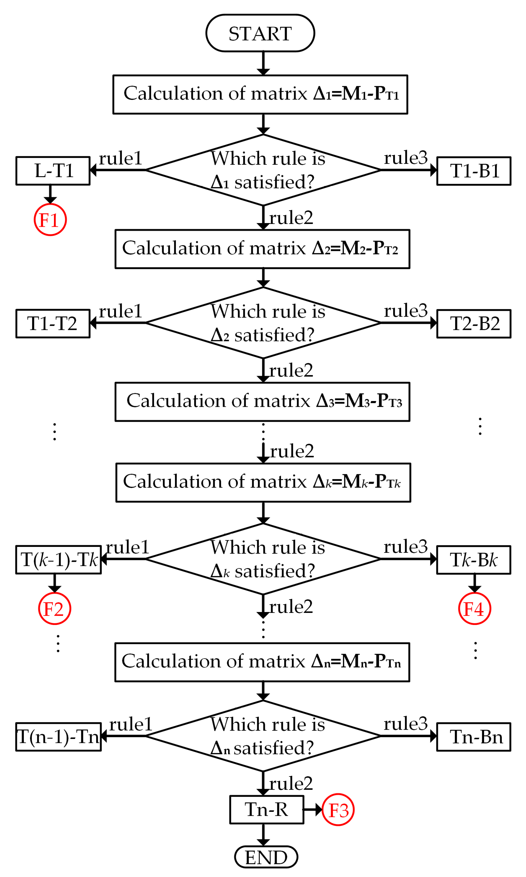
2.2. The Whole Scheme of Fault Section Identification in Multi-Terminal Lines

In this section, the rules for three-terminal lines are extended to locate fault sections in multi-terminal lines. A multi-terminal transmission line is depicted in Figure 5, and terminal L and terminal R are defined as the local terminal and remote terminal, respectively. The main line L–R has multiple tap nodes recorded as Tk (k = 1, 2, …, n). The line Tk–Bk is the corresponding branch line, where Bk denotes the kth terminal, except terminals L and R. The multi-terminal line can be seen as a superposed structure of n three-terminal lines with terminals L, R, Bk, and tap node Tk. Thus, the number of BDRM is n in the multi-terminal line, and the kth BDRM P_Tk is pre-calculated at the tap node Tk according to Equation (10), as follows:

$$P_{\mathrm{T}k}=\begin{array}{c}\begin{array}{ccc}\mathrm{L}& \mathrm{R}& \mathrm{B}k\end{array}\\ \begin{array}{c}\mathrm{L}\\ \mathrm{R}\\ \mathrm{B}k\end{array}\left[\begin{array}{ccc}1& l_{\mathrm{T}k\mathrm{L}}/l_{\mathrm{T}k\mathrm{R}}& l_{\mathrm{T}k\mathrm{L}}/l_{\mathrm{T}k\mathrm{B}k}\\ l_{\mathrm{T}k\mathrm{R}}/l_{\mathrm{T}k\mathrm{L}}& 1& l_{\mathrm{T}k\mathrm{R}}/l_{\mathrm{T}k\mathrm{B}k}\\ l_{\mathrm{T}k\mathrm{B}k}/l_{\mathrm{T}k\mathrm{L}}& l_{\mathrm{T}k\mathrm{B}k}/l_{\mathrm{T}k\mathrm{R}}& 1\end{array}\right]\end{array}$$

(15)

We assume that a fault occurs at an arbitrary position in the multi-terminal line. The arrival time differences of ground mode and aerial mode traveling waves are obtained from all terminals, and they are recorded as Δt_L, Δt_R, Δt_B1, Δt_B2, …, Δt_Bn. According to the process of building the FDRM, n FDRMs are built, and the kth FDRM M_k can be described as follows:

$$M_k=\begin{array}{c}\begin{array}{ccc}\mathrm{L}& \mathrm{R}& \mathrm{B}k\end{array}\\ \begin{array}{c}\mathrm{L}\\ \mathrm{R}\\ \mathrm{B}k\end{array}\left[\begin{array}{ccc}1& r_{\mathrm{LR}}& r_{\mathrm{LB}k}\\ 1/r_{\mathrm{LR}}& 1& r_{\mathrm{RB}k}\\ 1/r_{\mathrm{LB}k}& 1/r_{\mathrm{RB}k}& 1\end{array}\right]\end{array}$$

(16)

Then, the fault section identification method for multi-terminal lines is proposed according to different fault cases. Figure 5 shows all possible cases including F1-type fault points located in section L–T1, F2-type fault points located between two adjacent tap nodes T(k − 1) and Tk, F3-type fault points located in section Tn–R, and F4-type fault points in the branch line Tk–Bk. Figure 6 depicts the flowchart of the proposed method, the details of which are described next.

(1) F1-Type Fault Point between Terminal L and Tap Node T1

For an F1-type fault point, it is located in the three-terminal network with the terminals L, R, and B1, as well as the tap node T1. If the DRDM ∆₁ = M₁ − P_T1 is calculated and satisfies rule 1, the line L–T1 can be identified as the fault section.

(2) F2-Type Fault Point Located between Two Adjacent Tap Nodes T(k − 1) and Tk

For an F2-type fault point, the DRDM ∆₁ = M₁ − P_T1 is calculated first. In the three-terminal line with tap node T1, ∆₁ satisfies rule 2. Then, the DRDM ∆₂ = M₂ − P_T2 is calculated and judged. If ∆₂ satisfies rule 1, the line T1–T2 can be judged as a fault section. If ∆₂ still satisfies rule 2, the DRDMs ∆₃, ∆₄, …, ∆_k must be calculated and judged continuously during the process until ∆_k satisfies rule 1. Thus, the line T(k−1)–Tk can be judged as the fault section, if ∆₁, ∆₂, …, ∆_k−1 satisfy rule 2 and if ∆_k satisfies rule 1.

(3) F3-Type Fault Point Located in Section Tn–R

For an F3-type fault point, all the DRDMs ∆₁, ∆₂, …, ∆_n must be calculated and judged in a similar way. If all of them satisfy rule 2, the line Tn–R can be judged as the fault section.

(4) F4-Type Fault Point in the Branch Line Tk–Bk.

For an F4-type fault point, if the DRDM ∆_k satisfies rule 3, the branch line Tk–Bk can be judged as the fault section.

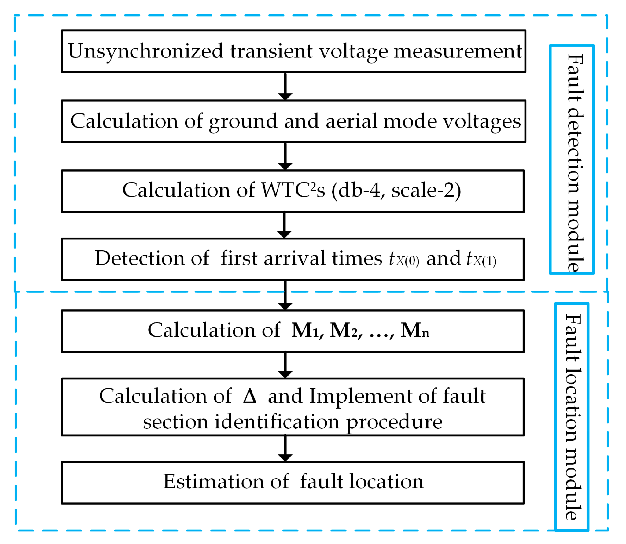
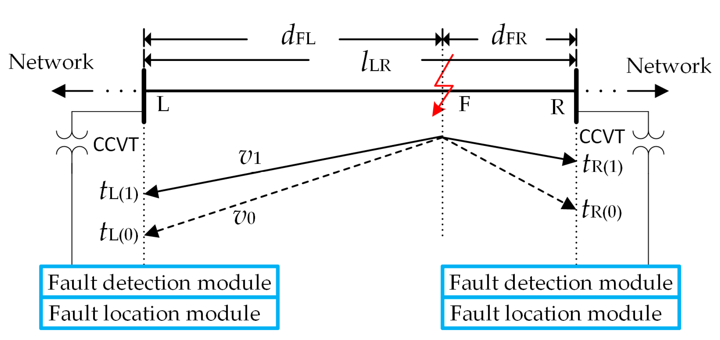
2.3. Fault Location Algorithm

After the fault section is identified according to the aforementioned method, the fault location can be determined by two terminals connecting each other through the fault section in the kth FDRM M_k. The fault distance can be obtained using the ratios related to the local terminal L in FDRM. The fault point in the main line and the fault point in the branch line can be calculated as follows:

$$d_{\mathrm{FL}-\mathrm{main}\mathrm{line}}=\frac{r_{\mathrm{LR}}}{1+r_{\mathrm{LR}}}{l}_{\mathrm{LR}}$$

(17)

$$d_{\mathrm{FL}-\mathrm{branch}\mathrm{line}}=\frac{r_{\mathrm{LB}k}}{1+r_{\mathrm{LB}k}}{l}_{\mathrm{LB}k}$$

(18)

where d_FL represents the distance of the fault to local terminal L. l_LR and l_LBk are the line lengths between two terminals connecting each other through the fault section.

Figure 7 shows the whole procedure of the proposed fault location method with the following steps:

Step 1: Fault-induced transient voltages at each terminal are collected without considering the data synchronization.

Step 2: Ground mode and aerial mode voltages are obtained using the Karrenbauer transformation.

Step 3: DWT with Daubechies-4 (db4) mother wavelet in scale-2 is used to calculate WTC²_S for the time-frequency decomposition of the mode voltages.

Step 4: The first arrival times of the ground mode (t_X(0)) and aerial mode (t_X(1)) at each terminal are obtained by marking the WTC²_S.

Step 5: A set of fault distance ratio matrixes M₁, M₂, …, M_n are calculated using (16).

Step 6: A series of distance ratio difference matrixes ∆₁, ∆₂, …, ∆_n are calculated and judged according to the identification procedure of the fault section. The procedure has been programmed. Once the fault section is found, the procedure will be terminated.

Step 7: Having identified the fault section, the fault location is estimated using (17) or (18).

In the following part, the test cases are simulated and the performance evaluations for the proposed method are presented.

3. Case Study and Performance Evaluation

To evaluate the proposed method, a five-terminal 220-kV/50-Hz transmission line in Figure 8 is simulated in PSCAD (PSCADX4.5, Manitoba HVDC Research Centre Inc., Winnipeg, MB, Canada) and MATLAB/Simulink (R2016a, MathWorks, Natick, MA, USA), and the distributed parameter model is adopted. The sampling frequency is 200 kHz. The related parameters of the simulated lines, together with the system, are taken from the Chinese northeast power system and listed in

Table 2. Parameters of simulated lines.

Parameters Type	Values
Source (p.u.)	EL = 1.04∠20°, EB1 = 1.02∠10°, EB3 = 1∠0°, ER = 0.98∠−10° EB3 = 1∠0°, ER = 0.98∠−10°
Lines	Z0 = 0.362 + j1.1426 (Ω/km), Y0 = j1.936 × 10−6 (S/km) Z1 = 0.035 + j0.4234 (Ω/km), Y1 = j2.726 × 10−6 (S/km)
Loads	Load1: 65 MW + 15 MVAR, Load2: 80 MW

. According to the line length parameters, the pre-calculated BDRMs have also been shown in

Table 3. Branch distance ratio matrixes (BDRMs) in simulated lines.

Line Length (km)	lT1L = 120, lT1T2 = 60, lT2T3 = 90, lT3R =30, lT1B1 = 80, lT2B2 = 50, lT3B3 = 100 lT1B1 = 80, lT2B2 = 50, lT3B3 = 100
BDRM	$P_{\mathrm{T}1}=\left[\begin{array}{ccc}1& 0.67& 1.50\\ -& 1& 2.25\\ -& -& 1\end{array}\right]$,$P_{\mathrm{T}2}=\left[\begin{array}{ccc}1& 1.5& 3.6\\ -& 1& 2.4\\ -& -& 1\end{array}\right]$, $P_{\mathrm{T}3}=\left[\begin{array}{ccc}1& 9& 2.7\\ -& 1& 0.3\\ -& -& 1\end{array}\right]$

. The fault location procedure is implemented according to the flowchart in Figure 7. To assess the accuracy of the proposed method, the fault location error is calculated as follows:

$$Err(\%)=\frac{\left|\mathrm{Estimated}\mathrm{distance}-\mathrm{Actual}\mathrm{distance}\right|}{\mathrm{Total}\mathrm{line}\mathrm{lengths}}\times 100\%$$

(19)

3.1. Description of a Test Case

As an example, an A-phase-to-ground (AG) in line section T2–T3 is used to illustrate the fault location procedure, which, in Figure 8, is at a distance of 265 km from terminal L, with a fault resistance of R_f = 50 Ω. According to steps 1 to 4, described in Section 2.3, the fault occurrence and feature extraction are presented in Figure 9. Figure 9a shows the three-phase voltage measured in terminal R before and during the fault. The image on the right (Figure 9b) is an enlarged view of the fault-induced distortion in the voltage waveform. The db4 mother wavelet shown in Figure 9c is selected for detected the fault-induced initial waves because of its wide use in fault-location literature and according to the investigations of different mother wavelets. Figure 9d shows the results of normalized WTC² and the arrival times of ground and aerial mode can be appreciated. To locate a fault, the time differences between the ground and aerial mode of the first traveling waves are measured at each terminal and shown in Figure 10.

According to Equations (6)–(9), the fault distance ratios and the FDRMs M₁, M₂, and M₃ in this case are obtained and listed in

Table 4. Fault distance ratios and fault distance ratio matrixes (FDRMs).

Fault Distance Ratio	rLR = 7.78, rLB1 = 1.19, rLB2 = 2.00, rLB3 = 2.50, rRB1 = 0.15, rRB2 = 0.26, rRB3 = 0.32 rRB1 = 0.16, rRB2 = 0.26, rRB3 = 0.33, lT1B1 = 80, lT2B2 = 50, lT3B3 = 100
FDRM	${\mathrm{M}}_1=\left[\begin{array}{ccc}1& 7.78& 1.19\\ -& 1& 0.15\\ -& -& 1\end{array}\right]$,${\mathrm{M}}_2=\left[\begin{array}{ccc}1& 7.78& 2\\ -& 1& 0.26\\ -& -& 1\end{array}\right]$,${\mathrm{M}}_3=\left[\begin{array}{ccc}1& 7.78& 2.5\\ -& 1& 0.32\\ -& -& 1\end{array}\right]$

. Thus, the difference matrix ∆₁ is calculated as follows:

$${\Delta }_1=M_1-P_{T1}\to \left[\begin{array}{ccc}0& >0& <0\\ -& 0& <0\\ -& -& 0\end{array}\right]$$

(20)

where ∆₁ satisfies rule 2, while the fault section identification procedure continues to execute, and ∆₂ is calculated as follows:

$${\Delta }_2=M_2-P_{T2}\to \left[\begin{array}{ccc}0& >0& <0\\ -& 0& <0\\ -& -& 0\end{array}\right]$$

(21)

where ∆₂ also satisfies rule 2, and ∆₃ is calculated as follows:

$${\Delta }_3=M_3-P_{T3}\to \left[\begin{array}{ccc}0& <0& <0\\ -& 0& >0\\ -& -& 0\end{array}\right]$$

(22)

where ∆₃ satisfies rule 1. According to the above procedure, the fault belongs to the F2-type fault point. Therefore, the line section T2–T3 is identified as the fault section. Because the line section T2–T3 is a part of the main line, the fault distance from the terminal L is calculated using (17), d_{FL-main line} = (7.78/(1 + 7.78) × 300 = 265.83 km. Finally, the fault location error related to this case is calculated using Err (%) = |265.83 − 265|/530 × 100% = 0.096%.

3.2. Perfomance Evaluation

In this section, many simulations have been done under different fault conditions. To better evaluate the accuracy of the proposed method, more fault points in different positions have also been tested. The satisfactory results of the fault section identification and fault location are included in

Table 5. Section identification and fault location in different positions.

Fault Location	lFL (km)	Fault Section	dFL (km)	Err (%)
5% of lT1L	6	L–T1	6.09	0.017
55% of lT1L	66	L–T1	65.84	0.030
95% of lT1L	114	L–T1	113.62	0.072
15% of lT1T2	129	T1–T2	128.57	0.081
45% of lT1T2	147	T1–T2	146.89	0.021
85% of lT1T2	171	T1–T2	171.45	0.085
10% of lT2T3	189	T2–T3	188.17	0.156
50% of lT2T3	225	T2–T3	225.40	0.075
90% of lT2T3	261	T2–T3	261.53	0.100
20% of lT3R	276	T3–R	276.57	0.107
40% of lT3R	282	T3–R	281.74	0.049
80% of lT3R	294	T3–R	293.90	0.019
5% of lT1B1	124	T1–B1	124.24	0.045
35% of lT1B1	148	T1–B1	147.63	0.070
75% of lT1B1	180	T1–B1	180.30	0.056
10% of lT2B2	185	T2–B2	183.97	0.194
30% of lT2B2	195	T2–B2	195.16	0.030
70% of lT2B2	215	T2–B2	214.77	0.043
5% of lT3B3	275	T3–B3	275.55	0.104

. It is concluded that the fault section can be correctly identified for an arbitrary position in the multi-terminal line. The fault location errors are relatively large near the tap nodes and the branch terminals, but the accuracy can meet the requirements of practical application.

To better assess the robustness of the proposed method, the simulations of test cases with various fault inception angles (FIAs) and fault resistance (R_f) are performed. The results of the fault location with the influence of the FIA and R_f are shown in

Table 6. Fault location error (Err%) for single-phase faults with influence of fault inception angle (FIA) and fault resistance.

FIA (°)	Rf (Ω)	F1-Type	F2-Type	F3-Type	F4-Type
		55% of lT1L	50% of lT2T3	40% of lT3R	65% of lT3B3
10	10	0.039	0.080	0.056	0.027
	50	0.041	0.083	0.059	0.030
	100	0.052	0.095	0.067	0.043
45	10	0.032	0.077	0.049	0.022
	50	0.035	0.079	0.053	0.026
	100	0.048	0.086	0.061	0.039
90	10	0.028	0.072	0.045	0.021
	50	0.030	0.075	0.049	0.023
	100	0.043	0.082	0.057	0.034

. Setting FIA as a constant, the errors increase with the increase in the fault resistance. Figure 11 shows that the proposed method can estimate the fault point more accurately when R_f ≤ 10 Ω. In addition, if the fault resistance remains constant, the fault location errors vary slightly with the FIA. The minimum fault location error exists at R_f = 10 Ω and FIA = 90°, and the fault location accuracy of the proposed method can be guaranteed. According to the above analysis, the proposed method is robust to FIAs and R_f. However, the application of the proposed method in different fault types is limited to grounded fault. The ground-mode component is approximate to zero when a phase-to-phase fault (ungrounded fault) occurs. In this situation, the arrival time of ground mode wave is difficult to detect. The method based on the arrival times of aerial and ground modes will fail to locate ungrounded fault. However, as far as one knows, ground faults are those that most likely take place in the power system (above 80%). Based on that, the proposed fault location method can also be widely used.

To show the advantages of the proposed method, it is compared with the existing method in the literature [23]. For a fair comparison, the benchmark dataset in a previous paper is used to evaluate these two methods. In addition, a line parameter error ε (ε is set as + 10% of the real line parameter) and GPS synchronized error δ (a 0.02 ms time delay is added at terminal R) are introduced into the simulations. The compared results are shown in

Table 7. Compared results of the two methods

Value	Sources of Errors		Method
	ε	δ	[23]	Proposed Method
Err (%)	-	-	0.082	0.075
	√	-	0.104	0.075
	-	√	8.936	0.075
	√	√	10.025	0.075

. The proposed method locates the fault as accurately as the existing method in the ideal case. However, after adding errors ε and δ, the proposed method presents better performances because ε can cause error in the velocities of calculation, and the unsynchronized data in the two-terminal method [23] can result in great fault location error in the previous method, but the accuracy of fault location in the proposed method is not affected by these system errors.

4. Conclusions

Traveling-wave-based fault location methods in multi-terminal topologies must be further improved. As little research has been done on the fault location of multi-terminal lines using the time difference of mode waves, a new fault location method for multi-terminal lines has been proposed in this paper. Using the time difference of mode waves, the distance ratio difference matrixes (DRDMs) are built, and the rules to identify the fault section have been presented. For the multi-terminal lines, the proposed method cannot be restricted by the multi-terminal time synchronization, and it is superior to that of other methods. Finally, the fault point can be estimated accurately in the fault section. The proposed method has been evaluated through test cases under different fault conditions. The simulation results have demonstrated the effectiveness and benefits of the proposed fault location method.

The advantage of the proposed fault location scheme is that the traveling wave recorders need not be restricted by time synchronization for multi-terminal lines. Further studies will focus on implementations of new fault location schemes with a limited number of measurement devices and diagnosis of multiple faults in complex networks.

References

1. Saha, M.M.; Izykowski, J.J.; Rosolowski, E. Fault Location on Power Networks, 1st ed.; Springer: New York, NY, USA, 2010. [Google Scholar]
2. Lopes, F.V.; Dantas, K.M.; Silva, K.M.; Costa, F.B. Accurate Two-terminal transmission line fault location using traveling waves. IEEE Trans. Power Deliv. 2017, 1, 873–880. [Google Scholar] [CrossRef]
3. Liu, C.W.; Lin, T.C.; Yu, C.S.; Yang, J.Z. Fault location technique for two-terminal multi-section compound transmission lines using synchronized phasor measurements. IEEE Trans. Smart Grid 2012, 3, 113–121. [Google Scholar] [CrossRef]
4. Das, S.; Santoso, S.; Gaikwad, A.; Patel, M. Impendence-based fault location in transmission network: Theory and application. IEEE Access 2014, 2, 537–557. [Google Scholar] [CrossRef]
5. Evrenosoglu, C.Y.; Abur, A. Travelling wave based fault location for teed circuits. IEEE Trans. Power Deliv. 2005, 20, 1115–1121. [Google Scholar] [CrossRef]
6. Lin, S.; He, Z.Y.; Li, X.P. Travelling wave time-frequency characteristic-based fault location method for transmission lines. IET Gener. Transm. Distrib. 2012, 6, 764–772. [Google Scholar] [CrossRef]
7. Gracia, J.; Mazon, A.J.; Zamora, I. Best ANN structures for fault location in single-and double-circuit transmission lines. IEEE Trans. Power Deliv. 2005, 20, 2389–2395. [Google Scholar] [CrossRef]
8. Swetapadma, A.; Yadav, A. A Novel Decision Tree Regression Based Fault Distance Estimation Scheme for Transmission Lines. IEEE Trans. Power Deliv. 2017, 32, 234–245. [Google Scholar] [CrossRef]
9. Ree, J.D.L.; Centeno, V.; Thorp, J.S.; Phadke, A.G. Synchronized Phasor Measurement Applications in Power Systems. IEEE Trans. Smart Grid 2010, 1, 20–27. [Google Scholar]
10. Dobakhshari, A.S.; Ranjbar, A.M. A Novel Method for Fault Location of Transmission Lines by Wide-Area Voltage Measurements Considering Measurement Errors. IEEE Trans. Smart Grid 2015, 6, 874–884. [Google Scholar] [CrossRef]
11. Wu, T.; Chung, C.Y.; Kamwa, I.; Li, J.; Qin, M. Synchrophasor measurement-based fault location technique for multi-terminal multi-section non-homogeneous transmission lines. IET Gener. Transm. Distrib. 2016, 10, 1815–1824. [Google Scholar] [CrossRef]
12. Mahamedi, B.; Sanaye-Pasand, M.; Azizi, S.; Zhu, J.G. Unsynchronised fault-location technique for three-terminal lines. IET Gener. Transm. Distrib. 2015, 9, 2099–2107. [Google Scholar] [CrossRef]
13. Hussain, S.; Osman, A.H. Fault location scheme for multi-terminal transmission lines using unsynchronized measurements. Int. J. Electr. Power Energy Syst. 2016, 78, 277–284. [Google Scholar] [CrossRef]
14. Personal, E.; García, A.; Parejo, A.; Larios, D.F.; Biscarri, F. A comparison of impedance-based fault location methods for power underground distribution systems. Energies 2016, 9, 1022. [Google Scholar] [CrossRef]
15. Argyropoulos, P.E.; Lev-Ari, H. Wavelet Customization for Improved Fault-Location Quality in Power Networks. IEEE Trans. Power Deliv. 2015, 30, 2215–2223. [Google Scholar] [CrossRef]
16. Lopes, F.V.; Fernandes, D.; Neves, W.L.A. A traveling-wave detection method based on Park’s transformation for fault locators. IEEE Trans. Power Deliv. 2013, 28, 1626–1634. [Google Scholar] [CrossRef]
17. Musa, M.H.H.; He, Z.Y.; Fu, L.; Deng, Y.J. Linear regression index-based method for fault detection and classification in power transmission line. IEE J. Trans. Electr. Electron. Eng. 2018, 13, 979–987. [Google Scholar] [CrossRef]
18. Gutten, M.; Korenciak, D.; Kucera, M.; Janura, R.; Glowacz, A.; Kantoch, E. Frequency and time fault diagnosis methods of power transformers. Meas. Sci. Rev. 2018, 18, 162–167. [Google Scholar] [CrossRef]
19. Da Silva, P.R.N.; Gabbar, H.A.; Vieira, P.; Da Costa, C.T. A new methodology for multiple incipient fault diagnosis in transmission lines using QTA and Naive Bayes classifier. Int. J. Electr. Power Energy Syst. 2018, 103, 326–346. [Google Scholar] [CrossRef]
20. Glowacz, A.; Glowacz, W.; Glowacz, Z. Recognition of armature current of DC generator depending on rotor speed using FFT, MSAF-1 and LDA. Eksploatacja i Niezawodność 2015, 17, 64–69. [Google Scholar] [CrossRef]
21. Silveira, E.G.; Paula, H.R.; Rocha, S.A.; Pereira, C.S. Hybrid fault diagnosis algorithms for transmission lines. Electr. Eng. 2018, 100, 1689–1699. [Google Scholar] [CrossRef]
22. Hamidi, R.J.; Livani, H.; Rezaiesarlak, R. Traveling-Wave Detection Technique using Short-Time Matrix Pencil Method. IEEE Trans. Power Deliv. 2017, 32, 2565–2574. [Google Scholar]
23. Costa, F.B. Fault-Induced Transient Detection Based on Real-Time Analysis of the Wavelet Coefficient Energy. IEEE Trans. Power Deliv. 2014, 29, 140–153. [Google Scholar] [CrossRef]
24. Shafiullah, M.; Abido, M.A. S-Transform based FFNN approach for distribution grids fault detection and classification. IEEE Access 2018, 6, 8080–8088. [Google Scholar] [CrossRef]
25. Mishra, P.K.; Yadav, A.; Pazoki, M.A. Novel Fault Classification Scheme for Series Capacitor Compensated Transmission Line Based on Bagged Tree Ensemble Classifier. IEEE Access 2018, 6, 27373–27382. [Google Scholar] [CrossRef]
26. Malik, H.; Sharma, R. Transmission line fault classification using modified fuzzy Q learning. IET Gener. Transm. Distrib. 2017, 11, 4041–4050. [Google Scholar] [CrossRef]
27. Chen, Y.Q.; Fink, O.; Sansavini, G. Combined fault location and classification for power transmission lines fault diagnosis with integrated feature extraction. IEEE Trans. Ind. Electron. 2018, 65, 561–569. [Google Scholar] [CrossRef]
28. Livani, H.; Evrenosoglu, C.Y. A fault classification and localization method for three-terminal circuits using machine learning. IEEE Trans. Power Deliv. 2013, 28, 2282–2290. [Google Scholar] [CrossRef]
29. Hamidi, R.J.; Livani, H. Traveling-Wave-Based Fault-Location Algorithm for Hybrid Multiterminal Circuits. IEEE Trans. Power Deliv. 2017, 32, 135–144. [Google Scholar] [CrossRef]
30. Zhu, Y.; Fan, X. Fault location scheme for a multi-terminal transmission line based on current traveling waves. Int. J. Electr. Power Energy Syst. 2013, 53, 367–374. [Google Scholar] [CrossRef]
31. Ning, Y.; Wang, D.Z.; Li, Y.L.; Zhang, H.X. Location of Faulty Section and Faults in Hybrid Multi-Terminal Lines Based on Traveling Wave Methods. Energies 2018, 11, 1105. [Google Scholar] [CrossRef]
32. Robson, S.; Haddad, A.; Griffiths, H. Fault location on branched networks using a multiended approach. IEEE Trans. Power Deliv. 2014, 29, 1955–1963. [Google Scholar] [CrossRef]
33. Lopes, F.V.; Silva, K.M.; Costa, F.B. Real-Time Traveling-Wave-Based Fault Location Using Two-Terminal Unsynchronized Data. IEEE Trans. Power Deliv. 2015, 30, 1067–1076. [Google Scholar] [CrossRef]
34. Liu, Y.; Sheng, G.; He, Z.; Jiang, X. A traveling wave fault location method for earth faults based on mode propagation time delays of multimeasuring points. Electrotech. Rev. 2012, 88, 254–258. [Google Scholar]
35. Liang, R.; Yang, Z.; Peng, N.; Liu, C.L.; Zare, F. Asynchronous Fault Location in Transmission Lines Considering Accurate Variation of the Ground-Mode Traveling Wave Velocity. Energies 2017, 10, 1957. [Google Scholar] [CrossRef]
36. Lopes, F.V. Setting-free traveling-wave-based earth fault location using unsynchronized two-terminal data. IEEE Trans. Power Deliv. 2016, 31, 2296–2298. [Google Scholar] [CrossRef]
37. Liang, R.; Wang, F.; Fu, G. Wide-area fault location based on optimal deployment of the traveling wave recorders. Int. Trans. Electr. Energy Syst. 2016, 26, 1661–1672. [Google Scholar] [CrossRef]
38. Liu, Y.; Sheng, G.; Hu, Y. Identification of lightning strike on 500-kV transmission line based on the time-domain parameters of a traveling Wave. IEEE Access 2016, 4, 7241–7250. [Google Scholar] [CrossRef]
39. Silva, C.A.; Fernandes, D.; Neves, W.L.A. Correction of the secondary voltage of coupling capacitor voltage transformers in real time. In Proceedings of the International Conference on Power Systems Transients (IPST 2011), Delft, The Netherlands, 14–17 June 2011. [Google Scholar]
40. Vermeulen, H.J.; Dann, L.R.; Rooijen, J.V. Equivalent circuit modelling of a capacitive voltage transformer for power system harmonic frequencies. IEEE Trans. Power Deliv. 1995, 10, 1743–1749. [Google Scholar] [CrossRef]
Figure 1. Traveling wave fault location network.
Energies 11 02957 g001
Figure 2. Time-space diagram for a line monitored at two terminals. CCVT—coupling capacitor voltage transformers.
Energies 11 02957 g002
Figure 3. Schematic diagram of wavelet decomposition.
Energies 11 02957 g003
Figure 4. Three-terminal line topology.
Energies 11 02957 g004
Figure 5. Diagram of a multi-terminal transmission line.
Energies 11 02957 g005
Figure 6. Flowchart of the proposed fault section identification method for multi-terminal transmission line.
Energies 11 02957 g006
Figure 7. Flowchart of the proposed fault location method. WTC2S—wavelet transformation coefficient squared.
Energies 11 02957 g007
Figure 8. Five-terminal lines simulation system.
Energies 11 02957 g008
Figure 9. A-phase-to-ground (AG) fault in 265 km from terminal L. (a) Three-phase voltage measured in terminal R before and during the fault; (b) The enlarged view of the fault-induced distortion waveform; (c) Daubechies-4 (db-4) mother wavelet; (d) The results of normalized WTC2.
Energies 11 02957 g009
Figure 10. WTC2 for ground and aerial mode waves and arrival time difference at each terminal. (a) Measured at terminal L; (b) Measured at terminal B1; (c) Measured at terminal B2; (d) Measured at terminal B3; (e) Measured at terminal R.
Energies 11 02957 g010
Figure 11. Influence of the fault resistance.
Energies 11 02957 g011