Effect of Energy and Failure Rate in a Multi-Item Smart Production System

Abstract

To form a smart production system, the effect of energy and machines’ failure rate plays an important role. The main issue is to make a smart production system for complex products that the system may produce several defective items during a long-run production process with an unusual amount of energy consumption. The aim of the model is to obtain the optimum amount of smart lot, the production rate, and the failure rate under the effect of energy. This study contains a multi-item economic imperfect production lot size energy model considering a failure rate as a system design variable under a budget and a space constraint. The model assumes an inspection cost to ensure product’s quality under perfect energy consumption. Failure rate and smart production rate dependent development cost under energy consumption are considered, i.e., lower values of failure rate give higher values of development cost and vice versa under the effect of proper utilization of energy. The manufacturing system moves from in-control state to out-of-control state at a random time. The theory of nonlinear optimization (Kuhn–Tucker method) is employed to solve the model. There is a lemma to obtain the global optimal solution for the model. Two numerical examples, graphical representations, and sensitivity analysis of key parameters are given to illustrate the model.

1. Introduction

During a long-run production, a common phenomenon is the production of defective items even though the production is considered under a smart manufacturing system under the consideration of proper energy consumption. The rate of production of defective items may be of two types: constant defective rate and random defective rate. In constant defective rate, the total number of defective items are fixed, whereas in random defective rate, the number of defective items varies based on several conditions of the production system. In reality, both defective rates are available constant defective rate (see for reference [1]) and random defective rate [2]. Until now, no author considered random defective rate for multi-item smart production under energy consideration with budget and space constraints. Though the major contribution is the concept of failure rate of a smart production system under energy consideration being introduced with the random time movement from in-control state to out-of-control state. The failure rate is defined as the total number of failures divided by total number of working hours. The failure rate of a smart production system is considered as a system reliability indicator because a lower failure rate indicates more reliable systems and a higher failure rate indicates less reliable systems. Therefore, the proposed model gives a new direction of random defective rate with an indication of system reliability for multi-item smart production and energy consumption with budget and space constraints. Usually, for any long-run production system, it may contain production of both perfect and imperfect products. The imperfect products can either be discarded or can be reworked to make them perfect. This imperfection occurs when the system moves to out-of-control state, which is due to the factors such as machine breakdown, program inaccuracy, machine operator’s inefficiency, and defective raw material supply. Several researchers have proposed inventory and production models with imperfect production systems. Kim and Hog [3] extended the Rossenblat and Lee [4] model within imperfect production systems by considering deteriorating production processes to obtain optimal production run length. They introduced the concept of system movement to out-of-control state from in-control state and producing defective items with three different deteriorating processes: constant, linearly increasing and exponentially increasing. Giri and Dohi [5] considered a random time of machine failure in an imperfect production system, where machine failure time and preventive time are random variables assuming stochastic machine breakdown and repair. They considered a net present value (NPV) approach for exact financial implications of the lot sizing to develop the EMQ model.

Sana et al. [6] extended the concept of an imperfect production system to introduce a new research dimension by considering a reduced selling-price for imperfect products. Reworking of the imperfect production items to make them as good as perfect quality items was introduced by Chiu et al. [7] and they proposed a model in which a portion of imperfect quality items is discarded, while the other portion is reworked by spending some costs. They optimized the finite production rate considering scrap production, reworking, and stochastic machine breakdown. The main research gap in this literature up to now is that no author utilized the concept of energy consumption and corresponding cost within any smart production system. Gonz$\acute{a}$lez et al. [8] developed a model on turbomachinery components which are using for grinding flank tools. Egea et al. [9] implemented a short-cut method to measure the available energy in a required load capacity of a forging machine. They estimated the total energy during the friction of two screws.

Sarkar [10] developed an inventory model for retailers with a stock-depended demand and delay-in-payments considering that the replenished items are not all perfect presuming that the production system is imperfect and the inventory is replenished at a finite rate. An important managerial insight was added by Sarkar [11] by introducing a time dependent rate of product deterioration in an inventory system, where an inventory replenishment rate is finite and the customer is offered quantity discounts to attract a large order size in order to maximize the profit. Production of imperfect items depends upon the system reliability. The greater the investment in system development to increase its reliability, the lesser the production of imperfect items will be. System reliability-dependent imperfect production was discussed by Sarkar [12] for an inflationary economic manufacturing quantity (EMQ) system, where demand depends upon the product price and advertisement. Chakraborty and Giri [13] modeled an imperfect production system, where system shifts to out-of-control state during preventive maintenance and, during the state, some imperfect items are produced, which are inspected and reworked at the end of the production run. They also assumed that some of the reworked items cannot be repaired.

An economic production quantity model with random defective rate of imperfect items’ production was investigated by Sarkar et al. [14] with rework process and planned backorders. They considered three different distribution density functions to calculate the rate of defective items and compared the results. Sarkar and Saren [15] studied deteriorating/imperfect production process, which randomly moves to an out-of-control state. They suggested that lot inspection policy should be adopted rather than full inspection policy to reduce the inventory costs. They also considered state of quality inspectors, who may falsely choose imperfect items as perfect and vice versa, which are designated as Type 1 and Type 2 errors. They also considered warranty policy over fixed time periods.

Pasandideh et al. [16] developed an inventory model for a multi-item single-machine lot size system with imperfect items’ production. Those imperfect items are further classified on the basis of their failure severity for reworking and scrap. They considered that product shortages are backlogged, in order to make it more realistic. Purohit et al. [17] conducted a comprehensive detailed analysis of a lot size problem, an inventory control system for non-stationary stochastic demand considering constraints of carbon emissions and cycle service level using carbon cap-and-trade regulatory mechanism. They generalized the study on effects of emission parameters and properties of product as well as the performance on supply chain. Due to involvement of labor in production and considering their influence on production of defective items, it is considered important to invest in personnel training according to the adopted system. Sana [18] investigated with production of defective items and developed an economic production lot size model with the environment of production system when it moves to out-of-control state. C$\acute{a}$rdenas-Barr$\acute{o}$n et al. [19] studies on optimal inventory with corrections and complements. Tiwari et al. [20,21] developed two models on deteriorating and partial backlogging.

Limited storage capacity for the inventory warehouse is now becoming a critical issue due to increasing costs of the storage facilities. This constraint is being considered by many researchers in situations where bulk production is being done. Huang et al. [22] developed an inventory model and investigated the optimal retailer’s lot sizing policy under partially permissible delay-in-payments and space constraints. They considered extra cost payment for rental warehouse, when the capacity of the existing warehouse is full. Pasandideh and Niaki [23] developed a nonlinear integer programming model to solve an inventory model considering multi-items with space limitations. They found the optimal solution of the model within the available warehouse space by adding a space constraint. Hafshejani et al. [24] solved a multi-stage inventory model with a nonlinear cost function and space constraint through a genetic algorithm. Mahapatra et al. [25] introduced an inventory model with demand and reliability dependent unit production cost under limited space availability. They supposed that available space is limited with fuzzy variable and solved the storage space goal using an intuitionistic fuzzy optimization technique.

The manufacturers have a limited budget and resources based on a periodic budget plan. Hence, consideration of budget constraints into the model is more realistic. Some researchers already analyzed budget constrained situations. For example, Mohan et al. [26] developed an optimal replenishment policy for multi-item ordering under conditions of permissible delay-in-payments, a budget constraint, and permissible partial-payment at a penalty. Hou and Lin [27] calculated the optimal lot size and optimal capital investment in setup costs with a limited capital budget to minimize the expected total annual cost and to reduce the yield variability for random yield. Taleizadeh et al. [28] studied a multi-item production system considering imperfect items and reworking thereof. They included a service level and a budget constraint within the model and calculated the global minimum. C$\acute{a}$rdenas-Barr$\acute{o}$n et al. [29] studied a production-inventory model in a just-in-time (JIT) system constrained with a maximum available budget and proposed a simple alternative heuristic algorithm to solve the model. Du et al. [30] and Todde et al. [31] developed models on energy analysis and energy consumption. Tomi$\acute{c}$ and Schneider [32] explained the method of how energy can be recovered from waste by a closed-loop. Haraldsson and Johansson [33] studied on measures of different types of energy efficiency during production. Xu et al. [34] discussed the production of bio-fuel oil from pyrolysis products of plants. This model is extended in the direction of energy. See

Table 1. Research contribution by several authors.

Author(s)	System Reliability	Development Cost	Energy	Defective Rate	Constraint Type	Item Type
Rosenblatt and Lee [4]	NA	NA	NA	Constant	NA	Single
Giri and Dohi [5]	NA	NA	NA	Random	NA	Single
Sana et al. [6]	NA	NA	NA	Random	NA	Single
Sarkar [12]	Variable	Variable	NA	Random	NA	Single
Sarkar and Saren [16]	NA	NA	NA	Random	NA	Single
Sana [18]	Variable	Variable	NA	Random	NA	Single
Taleizadeh et al. [28]	NA	NA	NA	Constant	Budget	Multiple
C$\acute{a}$rdenas-Barr$\acute{o}$n et al. [29]	NA	NA	NA	NA	Budget	Multiple
This paper	Variable	Variable	Considered	Random	Budget & Space	Multiple

NA indicates that is not applicable for that paper.

for the contribution of the different authors.

2. Problem Definition, Notation, and Assumptions

In this section, problem definition, notation and assumptions are given.

2.1. Problem Definition

A multi-item smart production system under an amount of energy consumption is considered with random defective items. At random time ${\tau }_i$, the system moves to out-of-control state from in-control state and produce defective items. The random time ${\tau }_i$ follows an exponential distribution (see, for instance, Sana [2]). To make the system more reliable under an appropriate consumption of energy, the development cost and unit production cost are assumed variable with respect to the failure rate of the system. The unit production cost also depends on the variable smart production rate. An inspection is considered to obtain the defective items as the system moves to out-of-control state. The defective items are reworked and transferred as perfect quality. The aim is to obtain maximum profit for a multi-item smart production system under the proper energy consumption by considering system failure rate and random defective rate (see Figure 1).

The following notation and assumptions are used to develop the model.

2.2. Assumptions

The following assumptions are considered to develop this model:

• The model consists of a multi-item smart production system with variable production rate under the perfect consumption of energy and it is greater than the demand (D) such that there is no shortage.
• The effect of energy is considered for the whole production system with an exact amount of energy consumption. The amount of energy consumption for holding inventory, inspection, rework, development, and tool/die cost is considered.
• During long-run production, at any random time ${\tau }_i$, the smart production system moves from in-control state to out-of-control state. The shifting time ${\tau }_i$ from in-control state to out-of-control state and the smart production rate follows a relation within them, where ${\tau }_i$ follows an exponential distribution by considering the failure rate $\eta$, which is a system design variable. If failure rate decreases, the system will be more reliable and, with the failure rate increasing, the system will be less reliable (see, for instance, Sarkar [12]).
• To increase the system reliability, the unit smart production cost is assumed as a sum of development cost, material cost and tool/die cost, where the development cost of products depends on the failure rate (see, for instance, Sana [2]) and amount of energy consumption.
• The model assumes multi-item smart production and there is a possibility of a space problem along with problem of total budget. The study considers space and budget constraints to solve these types of issues such that the model becomes more realistic (see for instance [28,29]) under the efficient energy consumption.
• In this model, although it is considered that the system will move to out-of-control state from in-control state after a certain time ${\tau }_i$, production disruption is not considered here (see for instance Sarkar and Saren [15]).
• The smart production system under energy consideration is considered for completely finished products. Work-in-process is not considered here.
• Lead time is assumed as negligible.

3. Mathematical Model

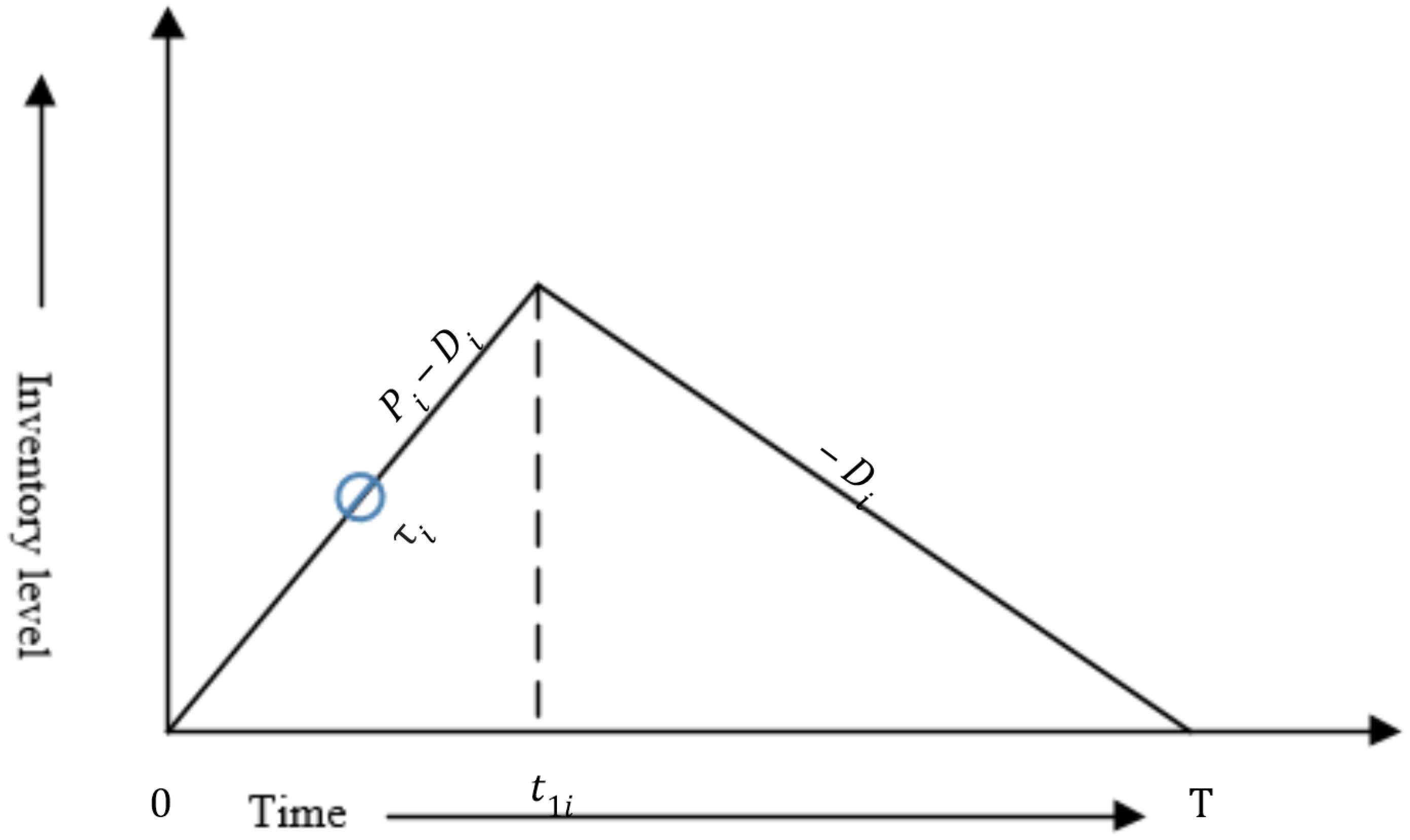
This study contains a production-inventory model with a multi-item under energy consideration. The smart production continues from $t_i=0$ to $t_i=t_{1i}$ for multi-item with a finite rate, where $t_i=Q_i/P_i$. The inventory piles up within the interval $[0,t_{1i}]$ and depletes within the interval $[t_{1i},T]$ with demand $D_i$. The model considers that, after a random time ${\tau }_i$, the system moves from in-control state to out-of-control state and produces imperfect products. See Figure 2 for the description of the production system.

The governing differential equation of the on-hand inventory is given by

$$\begin{array}{cc}\hfill \frac{d{I}_{1i}\left(t_i\right)}{d{t}_i}=& P_i-D_i,0\le t_i\le t_{1i},\hfill \\ \hfill & \mathrm{with}\mathrm{initial}\mathrm{condition}{I}_{1i}\left(0\right)=0,i=1,2,\dots ,n.\hfill \end{array}$$

(1)

$$\begin{array}{cc}\hfill \frac{d{I}_{2i}\left(t_i\right)}{d{t}_i}=& -D_i,t_{1i}\le t_i\le T,\hfill \\ \hfill & \mathrm{with}\mathrm{initial}\mathrm{condition}{I}_{2i}\left(T\right)=0,i=1,2,\dots ,n.\hfill \end{array}$$

(2)

The present state of inventories are given by

$$\begin{array}{cc}\hfill I_{1i}\left(t_i\right)=& (P_i-D_i)t_i,0\le t_i\le t_{1i},i=1,2,\dots ,n,\hfill \end{array}$$

(3)

$$\begin{array}{cc}\hfill I_{2i}\left(t_i\right)=& D_i(T-t_i),t_{1i}\le t_i\le T,i=1,2,\dots ,n.\hfill \end{array}$$

(4)

The model now considers the following costs to calculate the profit of the smart production system.

3.1. Setup Cost (SC)

Setup cost plays a very important role for multi-item smart production systems as each item contains a different setup system with different energy consumption. Thus, the model assumes that the setup cost for $ith$ item is considered as $C_{si}$ per setup with ${C_{si}}^{{}^{\prime }}$ as energy consumption cost per setup. Therefore, the average setup cost per unit cycle is

$$\begin{array}{cc}\hfill SC=& \sum _{i=1}^n(C_{si}+C_{si}^{{}^{\prime }})\frac{D_i}{Q_i}.\hfill \end{array}$$

3.2. Holding Cost (HC)

To calculate the holding cost for a smart multi-item production system, the average inventory for ith item has to calculate and, by taking summation over $i=1$ to n, one can obtain the total inventory over the cycle length of the smart production system. Therefore, the total inventory divided by the cycle length of the production cycle gives the average inventory and per unit holding cost multiplied by the average inventory gives the average holding cost per cycle.

Hence, for calculating the total inventory, one has

$$\begin{array}{cc}\hfill \mathrm{Inventory}=& \sum _{i=1}^n\left[{\int }_0^{t_{1i}}{I}_{1i}\left(t_i\right)d{t}_i+{\int }_{t_{1i}}^T{I}_{2i}\left(t_i\right)d{t}_i\right]\hfill \\ \hfill =& \sum _{i=1}^n\left[{\int }_0^{t_{1i}}(P_i-D_i)t_{i}d{t}_i+{\int }_{t_{1i}}^T{D}_i(T-t_i)d{t}_i\right].\hfill \end{array}$$

As energy consumption is calculated with the appropriate costs, the holding cost for average inventory per unit time under the presence of cost for energy consumption is

$$\begin{array}{cc}\hfill HC=& \sum _{i=1}^n\frac{(C_{hi}+C_{hi}^{{}^{\prime }})D_i}{2Q_i}\left[{\int }_0^{t_{1i}}(P_i-D_i)t_{i}d{t}_i+{\int }_{t_{1i}}^T\left\{(P_i-D_i){\frac{Q_i}{P}}_i-D_i{t}_i\right\}d{t}_i\right]\hfill \\ \hfill =& \sum _{i=1}^n\frac{(C_{hi}+C_{hi}^{{}^{\prime }})Q_i}{2}\left(1-\frac{D_i}{P_i}\right).\hfill \end{array}$$

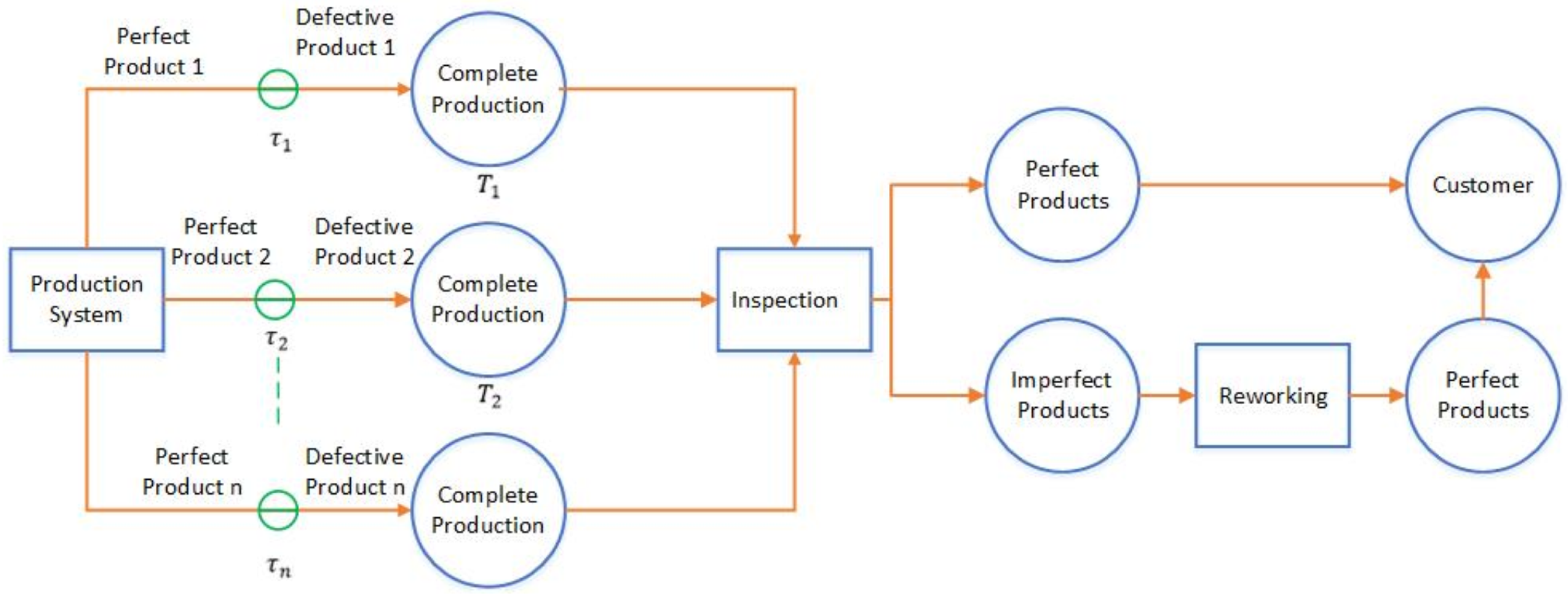
3.3. Inspection Cost (IC)

During a long-run process, the smart production system may move to out-of-control state, thus an inspection of each product is necessary. By inspection, the industry can assure the good quality of products, which generally maintain the brand image of the industry. If inspection cost per unit is $C_i$ and $C_i^{\prime }$ is the cost per unit for energy consumed due to inspection, then the inspection cost per unit cycle under energy consideration is

$$\begin{array}{cc}\hfill IC=& \sum _{i=1}^n(C_i+C_i^{{}^{\prime }})Q_i\times \frac{D_i}{Q_i}\hfill \\ \hfill =& \sum _{i=1}^n(C_i+C_i^{{}^{\prime }})D_i.\hfill \end{array}$$

3.4. Rework Cost (RC)

After inspection of each product, those items, detected as defective, are considered for reworking to make them as if they are perfect. To calculate the rework cost, the number of defective items and the rate of defective items production are needed.

The rate of defective items $g(t_i,{\tau }_i,P_i)$ is considered (see, for instance, [2]) as

$$\begin{array}{cc}\hfill g(t_i,{\tau }_i,P_i)=& \alpha P_i^{\beta }{(t_i-{\tau }_i)}^{\gamma },\mathrm{where}\beta \ge 0,\gamma \ge 0\mathrm{and}{t}_i\ge {\tau }_i.\hfill \end{array}$$

(5)

There is a quality level of smart production defined by the management system of the smart production industry, below which a product will not remain qualitative. The items that do not qualify the requirements of quality are imperfect items and cannot be forwarded to customers before reworking. The production system produces defective from random time ${\tau }_i$ till time $t_{1i}$, which is the time for maximum inventory.

There is no imperfect items within the interval $[0,{\tau }_i]$ and all imperfect items produce within $[{\tau }_i,t_{1i}]$. Thus, number of imperfect items within the interval $[{\tau }_i,t_{1i}]$ is

$$\begin{array}{cc}\hfill N=& P_i{\int }_{{\tau }_i}^{t_{1i}}\alpha P_i^{\beta }{(t_i-{\tau }_i)}^{\gamma }dt\hfill \\ \hfill =& \left(\frac{\alpha }{\gamma +1}\right)P_i^{\beta +1}{(t_{1i}-{\tau }_i)}^{\gamma +1}.\hfill \end{array}$$

(6)

Therefore, the number of imperfect items within the full cycle is

$$\begin{array}{cc}\hfill N=& \left\{\begin{array}{c}0,\mathrm{if}{\tau }_i\ge t_{1i},\hfill \\ \left(\frac{\alpha }{\gamma +1}\right)P_i^{\beta +1}{(t_{1i}-{\tau }_i)}^{\gamma +1},\mathrm{if}{\tau }_i\le t_{1i},\hfill \end{array}\right.\hfill \end{array}$$

where the random time ${\tau }_i$ follows the exponential distribution.

The distribution function of ${\tau }_i$ within the out-of-control state is considered as

$$\begin{array}{c}\hfill G\left({\tau }_i\right)=1-e^{-\eta {\tau }_i},\end{array}$$

(7)

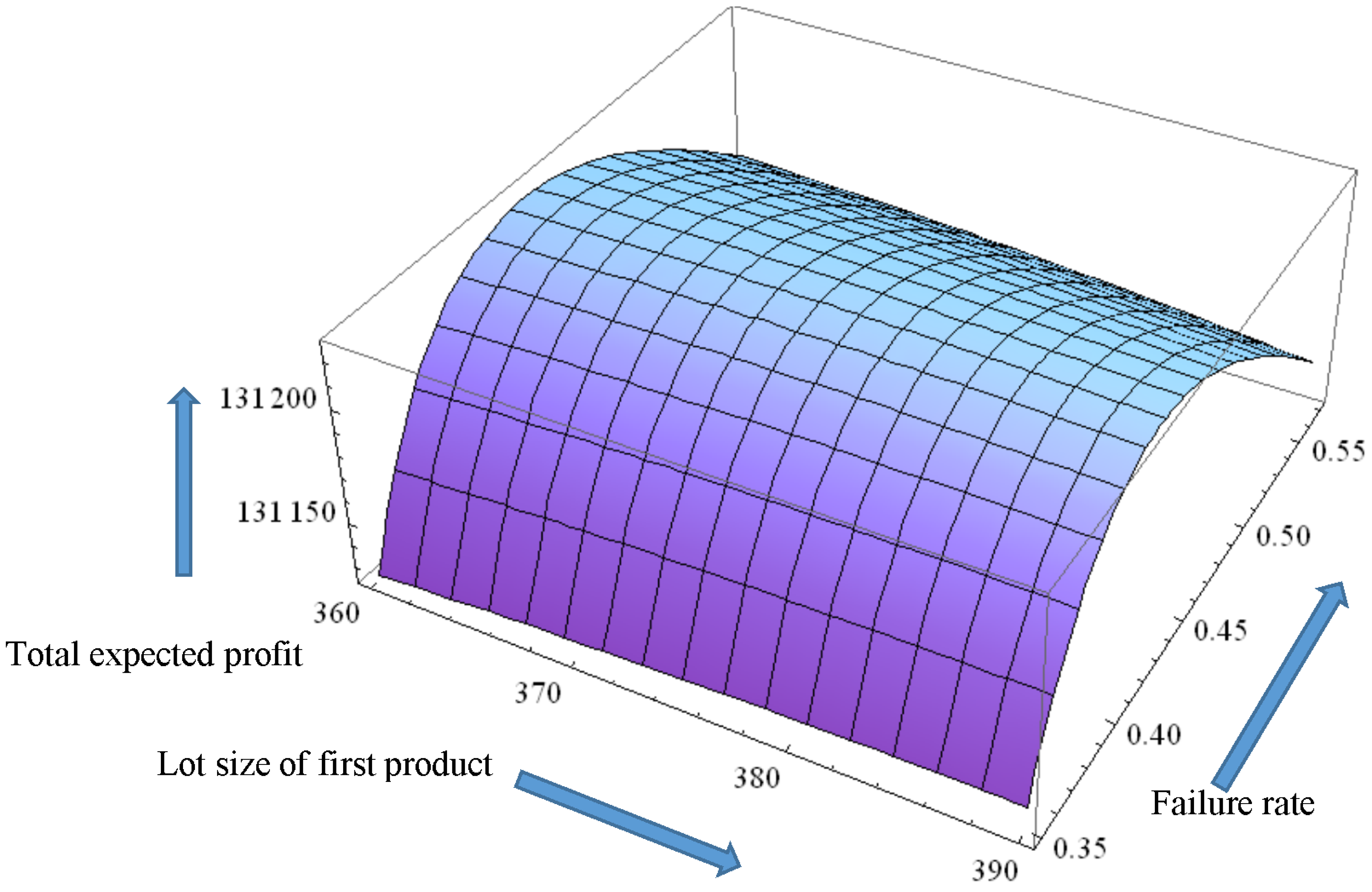
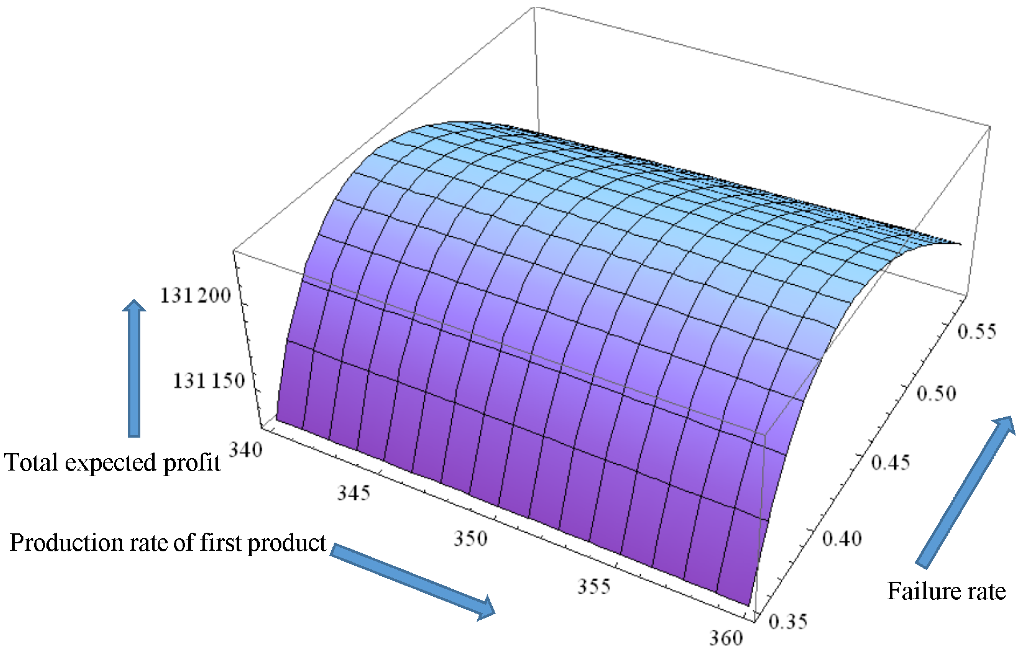
where $\eta$ is the failure rate, known as system design variable. The lower value of $\eta$ indicates a higher value of system reliability. Now, to ensure the distribution function, it can be found easily

$$\begin{array}{cc}\hfill {\int }_0^{\infty }dG\left({\tau }_i\right)=& 1.\hfill \end{array}$$

Generally, the rate of defective items’ production cannot be determined. However, on the basis of previous data, an expected number of defective items’ production can be calculated. We are adding those expected number of produced defective items to calculate the cost of imperfect products. Thus, the density function for the random time ${\tau }_i$ has to consider for calculation of the expected number of defective items within a full cycle. Hence, the expected number of imperfect items for the full cycle is

$$\begin{array}{cc}\hfill E\left(N\right)=& \sum _{i=1}^n\left(\frac{\alpha }{\gamma +1}\right)P_i^{\beta +1}{\int }_0^{t_{1i}}{(t_{1i}-{\tau }_i)}^{\gamma +1}dG\left({\tau }_i\right)\hfill \\ \hfill =& \sum _{i=1}^n\eta P_i^{\beta +1}\left(\frac{\alpha }{\gamma +1}\right)e^{\frac{-\eta Q_i}{P_i}}\psi \left(\eta ,\frac{Q_i}{P_i}\right),\mathrm{as}{t}_{1i}=\frac{Q_i}{P_i}.\hfill \end{array}$$

(8)

To change the status of defective products, the rework cost along with the cost for energy consumption during reworking is used to make them perfect as new. The rework cost per unit cycle (RC) is

$$\begin{array}{cc}\hfill RC=& \sum _{i=1}^n(R_i+R_i^{{}^{\prime }})\frac{D_i}{Q_i}E\left(N\right).\hfill \end{array}$$

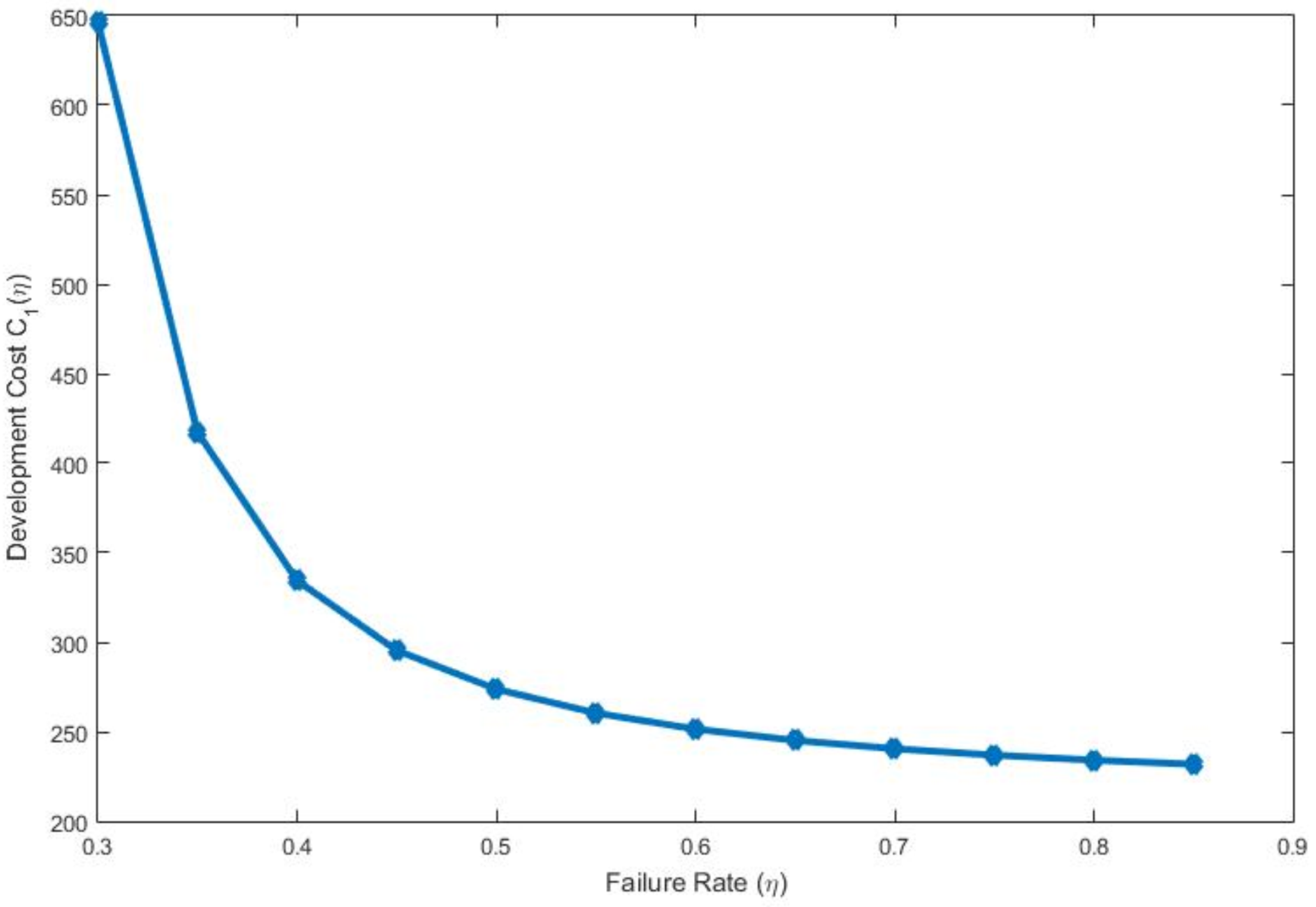
3.5. Development Cost (DC)

To make the system more reliable, the failure rate, which in turn indicates the system reliability, is considered within the development cost of products. The labor cost and energy resource cost are included within it. Thus, the development cost per unit time is considered as

$$\begin{array}{ccc}\hfill C_1\left(\eta \right)& =\hfill & \hfill M+X{e}^{r\frac{{\eta }_{max}-\eta }{\eta -{\eta }_{min}}}.\end{array}$$

(9)

3.6. Unit Production Cost (UPC)

Unit production cost is considered as the sum of raw material cost per product, development cost per product and tool/die cost. The unit production is directly proportional to the material cost as the increasing raw material cost indicates the increasing value of the unit production cost. It is also directly proportional to development cost and tool/die cost, as increasing the value of these costs results in more unit production cost. Unit production cost per unit time is assumed as

$$\begin{array}{ccc}\hfill C_p(\eta ,P_i)& =\hfill & \hfill \sum _{i=1}^n\left[C_m+\frac{C_1\left(\eta \right)}{P_i}+{\alpha }_1{P}_i^{\delta }\right],\end{array}$$

(10)

where $C_m$ is the material cost per unit item, whose quality helps to make the system more reliable. $C_1\left(\eta \right)$ is the development cost which depends on failure rate $\eta$. With the increasing percentage of failure rate, the development cost increases, which indicates more reliable system as $\eta$, the failure rate, indicates the system reliability, and, when it decreases, development cost decreases. $\alpha P_i^{\delta }(\delta >0)$ is the tool/die cost.

3.7. Expected Total Profit (ETP)

The expected total profit per unit cycle is ETP ($Q_i,P_i,\eta$) = Revenue−HC−SC−IC−RC

$$\begin{array}{cc}\hfill ETP(Q_i,P_i,\eta )=& \sum _{i=1}^n[D_i(W_i-C_p)-\frac{(C_{hi}+C_{hi}^{{}^{\prime }})Q_i}{2}\left(1-\frac{D_i}{P_i}\right)-(C_{si}+C_{si}^{{}^{\prime }})\frac{D_i}{Q_i}\hfill \\ \hfill -& (C_i+C_i^{{}^{\prime }})D_i-(R_i+R_i^{{}^{\prime }})\left(\frac{D_i\alpha }{Q_i(\gamma +1)}\right)P_i^{\beta +1}\eta e^{\frac{-\eta Q_i}{P_i}}\psi \left(\eta ,\frac{Q_i}{P_i}\right)],\hfill \end{array}$$

(11)

as $t_{2i}=\frac{(P_i-D_i)Q_i}{P_i{D}_i}$, (see Appendix A for the value of $\psi \left(\eta ,\frac{Q_i}{P_i}\right)$).

3.8. Constraints

In any business system, investment is not unlimited. With the available capital, a manufacturer can buy the plausible combinations of materials and services to satisfy the demand of its customer. Similarly, in an imperfect production system, only a specific percentage of budget can be allocated for inspection and reworking of imperfect items. There is a certain quality level, below which the threshold of the allocated budget is crossed and that imperfect item will not be reworked. This model considers a budget constraint and the managers define a specific quality level/threshold quality level to separate the imperfect products, which can be reworked or not chosen for reworking. Like budget, space is also a constraint in any type of production system. Excess inventory and space are used and trigger additional costs and thus the aims to eliminate excess space and inventory. For an imperfect production system, a limited space is allocated to store and rework the imperfect production.

Thus, considering budget and space constrains, the profit equation becomes

$$\begin{array}{cc}\hfill ETP(Q_i,P_i,\eta )=& \sum _{i=1}^n[D_i(W_i-C_p)-\frac{(C_{hi}+C_{hi}^{{}^{\prime }})Q_i}{2}\left(1-\frac{D_i}{P_i}\right)-(C_{si}+C_{si}^{{}^{\prime }})\frac{D_i}{Q_i}\hfill \\ \hfill -& (C_i+C_i^{{}^{\prime }})D_i-(R_i+R_i^{{}^{\prime }})\left(\frac{D_i\alpha }{Q_i(\gamma +1)}\right)P_i^{\beta +1}\eta e^{\frac{-\eta Q_i}{P_i}}\psi \left(\eta ,\frac{Q_i}{P_i}\right)],\hfill \\ \hfill & \mathrm{subject}\mathrm{to}\hfill \\ \hfill & \sum _{i=1}^n{\xi }_i{Q}_i\le A,\hfill \\ \hfill & \sum _{i=1}^n{\varphi }_i{Q}_i\le B,\hfill \end{array}$$

(12)

where the first term indicates revenues, the second term gives the holding cost and energy consumption cost due to holding products, the third term provides a setup cost and energy consumption of setup cost, the fourth term indicates inspection cost and energy utilization cost for inspection, the fifth cost is for reworking and the use of energy cost for reworking, and the next two terms are for space and budget constraints.

To obtain the maximum profit with respect to the optimum production quantity, production rate, and failure rate, the model has to solve with the best solution approach, which is described in the next section.

4. Solution Methodology

The profit function is highly nonlinear and it contains inequality constraints. Thus, the Kuhn–Tucker method is the best approach to solve this model.

Therefore, using the Kuhn–Tucker condition, the solution can be obtained as follows:

Lagrange equation of the above profit function is given by

$$\begin{array}{cc}\hfill L(Q_i,P_i,\eta ,{\lambda }_1,{\lambda }_2)=& \sum _{i=1}^n[D_i(W_i-C_p)-\frac{(C_{hi}+C_{hi}^{{}^{\prime }})Q_i}{2}\left(1-\frac{D_i}{P_i}\right)-(C_{si}+C_{si}^{{}^{\prime }})\frac{D_i}{Q_i}\hfill \\ \hfill -& (C_i+C_i^{{}^{\prime }})D_i-\frac{\eta {\zeta }_1{P}_i^{\beta +1}}{Q_i}{e}^{\frac{-\eta Q_i}{P_i}}\psi \left(\eta ,\frac{Q_i}{P_i}\right)+{\lambda }_1({\xi }_i{Q}_i-A)\hfill \\ \hfill +& {\lambda }_2({\varphi }_i{Q}_i-B)],\hfill \end{array}$$

where ${\lambda }_1$ and ${\lambda }_2$ are Lagrange multiplier and ${\zeta }_1=\frac{\alpha R_i{D}_i}{\gamma +1}$.

From the necessary condition of optimization of the Kuhn–Tucker method, one can obtain

$$\begin{array}{cc}\hfill \frac{\partial L}{\partial Q_i}=& -\frac{(C_{hi}+C_{hi}^{{}^{\prime }})}{2}\left(1-\frac{D_i}{P_i}\right)+\frac{(C_{si}+C_{si}^{{}^{\prime }})D_i}{Q_i^2}+\frac{\eta {\zeta }_1{P}_i^{\beta +1}}{Q_i}{e}^{\frac{-\eta Q_i}{P_i}}\psi \left(\eta ,\frac{Q_i}{P_i}\right)\hfill \\ \hfill +& \frac{{\eta }^2{\zeta }_1{P}_i^{\beta }}{Q_i}{e}^{\frac{-\eta Q_i}{P_i}}\psi \left(\eta ,\frac{Q_i}{P_i}\right)-\frac{\eta {\zeta }_1{P}_i^{\beta +1}}{Q_i}{e}^{\frac{-\eta Q_i}{P_i}}\frac{\partial \psi }{\partial Q_i}+{\lambda }_1{\xi }_i+{\lambda }_2{\varphi }_i\ge 0,\hfill \end{array}$$

(13)

$$\begin{array}{cc}\hfill \frac{\partial L}{\partial P_i}=& \frac{D_i{C}_1\left(\eta \right)}{P_i^2}-D_i({\alpha }_1+{\alpha }_1^{{}^{\prime }})\delta P_i^{\delta -1}-\frac{(C_{hi}+C_{hi}^{{}^{\prime }})D_i{Q}_i}{2P_i^2}-\frac{\eta {\zeta }_1(\beta +1)P_i^{\beta }}{Q_i}{e}^{\frac{-\eta Q_i}{P_i}}\psi \left(\eta ,\frac{Q_i}{P_i}\right)\hfill \\ \hfill -& \frac{{\eta }^2{\zeta }_1}{P_i^2}{e}^{\frac{-\eta Q_i}{P_i}}\psi \left(\eta ,\frac{Q_i}{P_i}\right)-\frac{\eta {\zeta }_1{P}_i^{\beta +1}}{Q_i}{e}^{\frac{-\eta Q_i}{P_i}}\frac{\partial \psi }{\partial P_i}\ge 0,\hfill \end{array}$$

(14)

$$\begin{array}{cc}\hfill \frac{\partial L}{\partial \eta }=& \frac{D_{i}Nr({\eta }_{max}-{\eta }_{min})}{P_i{(\eta -{\eta }_{min})}^2}{e}^{\frac{r({\eta }_{max}-\eta )}{\eta -{\eta }_{min}}}-\frac{{\zeta }_1{P}_i^{\beta +1}}{Q_i}{e}^{\frac{-\eta Q_i}{P_i}}\psi \left(\eta ,\frac{Q_i}{P_i}\right)\hfill \\ \hfill +& \frac{\eta {\zeta }_1{P}_i^{\beta }}{Q_i}{e}^{\frac{-\eta Q_i}{P_i}}\psi \left(\eta ,\frac{Q_i}{P_i}\right)-\frac{\eta {\zeta }_1{P}_i^{\beta +1}}{Q_i}{e}^{\frac{-\eta Q_i}{P_i}}\frac{\partial \psi }{\partial \eta }\ge 0.\hfill \end{array}$$

(15)

From the Kuhn–Tucker condition, one can write

$$\begin{array}{cc}\hfill & \frac{(C_{si}+C_{si}^{{}^{\prime }})D_i}{Q_i^2}+\frac{\eta {\zeta }_1{P}_i^{\beta +1}}{Q_i}{e}^{\frac{-\eta Q_i}{P_i}}\psi \left(\eta ,\frac{Q_i}{P_i}\right)-\frac{(C_{hi}+C_{hi}^{{}^{\prime }})}{2}\left(1-\frac{D_i}{P_i}\right)\hfill \\ \hfill & +\frac{{\eta }^2{\zeta }_1{P}_i^{\beta }}{Q_i}{e}^{\frac{-\eta Q_i}{P_i}}\psi \left(\eta ,\frac{Q_i}{P_i}\right)-\frac{\eta {\zeta }_1{P}_i^{\beta +1}}{Q_i}{e}^{\frac{-\eta Q_i}{P_i}}\frac{\partial \psi }{\partial Q_i}+{\lambda }_1{\xi }_i+{\lambda }_2{\varphi }_i=0,\hfill \end{array}$$

(16)

$$\begin{array}{cc}\hfill & \frac{D_i{C}_1\left(\eta \right)}{P_i^2}-D_i({\alpha }_1+{\alpha }_1^{{}^{\prime }})\delta P_i^{\delta -1}-\frac{(C_{hi}+C_{hi}^{{}^{\prime }})D_i{Q}_i}{2P_i^2}-\frac{\eta {\zeta }_1(\beta +1)P_i^{\beta }}{Q_i}{e}^{\frac{-\eta Q_i}{P_i}}\psi \left(\eta ,\frac{Q_i}{P_i}\right)\hfill \\ \hfill & -\frac{{\eta }^2{\zeta }_1}{P_i^2}{e}^{\frac{-\eta Q_i}{P_i}}\psi \left(\eta ,\frac{Q_i}{P_i}\right)-\frac{\eta {\zeta }_1{P}_i^{\beta +1}}{Q_i}{e}^{\frac{-\eta Q_i}{P_i}}\frac{\partial \psi }{\partial P_i}=0,\hfill \end{array}$$

(17)

$$\begin{array}{cc}\hfill & \frac{D_{i}Nr({\eta }_{max}-{\eta }_{min})}{P_i{(\eta -{\eta }_{min})}^2}{e}^{\frac{r({\eta }_{max}-\eta )}{\eta -{\eta }_{min}}}-\frac{{\zeta }_1{P}_i^{\beta +1}}{Q_i}{e}^{\frac{-\eta Q_i}{P_i}}\psi \left(\eta ,\frac{Q_i}{P_i}\right)\hfill \\ \hfill & +\frac{\eta {\zeta }_1{P}_i^{\beta }}{Q_i}{e}^{\frac{-\eta Q_i}{P_i}}\psi \left(\eta ,\frac{Q_i}{P_i}\right)-\frac{\eta {\zeta }_1{P}_i^{\beta +1}}{Q_i}{e}^{\frac{-\eta Q_i}{P_i}}\frac{\partial \psi }{\partial \eta }=0.\hfill \end{array}$$

(18)

To show the global optimality of the profit function, the sufficient condition from the Kuhn–Tucker condition must be satisfied. To obtain the global optimal solution, a lemma is established as follows:

Lemma 1. 

(i) If ${\zeta }_2>0$, ${\zeta }_2{\zeta }_3-{\left({\zeta }_5\right)}^2<0$, $({\zeta }_2{\zeta }_3{\zeta }_4-{\zeta }_2{\zeta }_7^2-{\zeta }_5^2{\zeta }_4+2{\zeta }_5{\zeta }_6{\zeta }_7-{\zeta }_6^2{\zeta }_3)>0$ or (ii) ${\zeta }_2<0$, ${\zeta }_2{\zeta }_3-{\left({\zeta }_5\right)}^2>0$, $({\zeta }_2{\zeta }_3{\zeta }_4-{\zeta }_2{\zeta }_7^2-{\zeta }_5^2{\zeta }_4+2{\zeta }_5{\zeta }_6{\zeta }_7-{\zeta }_6^2{\zeta }_3)<0$ then $L(Q_i,P_i,\eta ,{\lambda }_1,{\lambda }_2)$ at $(Q_i^{*},P_i^{*},{\eta }^{*})$ will be maximum, when

$$\begin{array}{c}-\frac{(C_{hi}+C_{hi}^{{}^{\prime }})}{2}\left(1-\frac{D_i}{P_i}\right)+\frac{(C_{si}+C_{si}^{{}^{\prime }})D_i}{{\left(Q_i^{*}\right)}^2}+\frac{\eta {\zeta }_1{P}_i^{\beta +1}}{Q_i^{*}}{e}^{\frac{-\eta Q_i^{*}}{P_i}}\psi \left(\eta ,\frac{Q_i^{*}}{P_i}\right)+\frac{{\eta }^2{\zeta }_1{P}_i^{\beta }}{Q_i^{*}}{e}^{\frac{-\eta Q_i^{*}}{P_i}}\psi \left(\eta ,\frac{Q_i^{*}}{P_i}\right)\hfill \\ -\frac{\eta {\zeta }_1{P}_i^{\beta +1}}{Q_i^{*}}{e}^{\frac{-\eta Q_i^{*}}{P_i}}\frac{\partial \psi }{\partial Q_i^{*}}+{\lambda }_1{\xi }_i+{\lambda }_2{\varphi }_i=0,\frac{-(C_{hi}+C_{hi}^{{}^{\prime }})D_i{Q}_i}{2{\left(P_i^{*}\right)}^2}-\frac{\eta {\zeta }_1(\beta +1){\left(P_i^{*}\right)}^{\beta }}{Q_i}{e}^{\frac{-\eta Q_i}{P_i^{*}}}\psi \left(\eta ,\frac{Q_i}{P_i^{*}}\right)\hfill \\ -\frac{{\eta }^2{\zeta }_1}{{\left(P_i^{*}\right)}^2}{e}^{\frac{-\eta Q_i}{P_i^{*}}}\psi \left(\eta ,\frac{Q_i}{P_i^{*}}\right)-\frac{\eta {\zeta }_1{\left(P_i^{*}\right)}^{\beta +1}}{Q_i}{e}^{\frac{-\eta Q_i}{P_i^{*}}}\frac{\partial \psi }{\partial P_i^{*}}=0,and-\frac{{\zeta }_1{P}_i^{\beta +1}}{Q_i}{e}^{\frac{-{\eta }^{*}{Q}_i}{P_i}}\psi \left({\eta }^{*},\frac{Q_i}{P_i}\right)\hfill \\ +\frac{{\eta }^{*}{\zeta }_1{P}_i^{\beta }}{Q_i}{e}^{\frac{-{\eta }^{*}{Q}_i}{P_i}}\psi \left({\eta }^{*},\frac{Q_i}{P_i}\right)-\frac{{\eta }^{*}{\zeta }_1{P}_i^{\beta +1}}{Q_i}{e}^{\frac{-{\eta }^{*}{Q}_i}{P_i}}\frac{\partial \psi }{\partial {\eta }^{*}}=0.\hfill \end{array}$$

Proof. 

To find the sufficient condition of the global optimality, taking 2nd order derivatives of Equations (13)–(15) with respect to $Q_i$, $P_i$, and $\eta$, it becomes

$$\begin{array}{cc}\hfill \frac{{\partial }^{2}L}{\partial {Q_i}^2}=& -\frac{2(C_{si}+C_{si}^{{}^{\prime }})D_i}{Q_i^3}-\frac{2\eta {\zeta }_1{P}_i^{\beta +1}}{Q_i^3}{e}^{\frac{-\eta Q_i}{P_i}}\psi \left(\eta ,\frac{Q_i}{P_i}\right)-\frac{2{\eta }^2{\zeta }_1{P}_i^{\beta }}{Q_i^2}{e}^{\frac{-\eta Q_i}{P_i}}\psi \left(\eta ,\frac{Q_i}{P_i}\right)\hfill \\ \hfill +& \frac{2\eta {\zeta }_1{P}_i^{\beta +1}}{Q_i^2}{e}^{\frac{-\eta Q_i}{P_i}}\frac{\partial \psi }{\partial Q_i}-\frac{{\eta }^3{\zeta }_1{P}_i^{\beta -1}}{Q_i}{e}^{\frac{-\eta Q_i}{P_i}}\psi \left(\eta ,\frac{Q_i}{P_i}\right)+\frac{2{\eta }^2{\zeta }_1{P}_i^{\beta }}{Q_i}{e}^{\frac{-\eta Q_i}{P_i}}\frac{\partial \psi }{\partial Q_i}\hfill \\ \hfill -& \frac{\eta {\zeta }_1{P}_i^{\beta +1}}{Q_i}{e}^{\frac{-\eta Q_i}{P_i}}\frac{{\partial }^2\psi }{\partial Q_i^2}\hfill \\ \hfill =& {\zeta }_2\left(\mathrm{say}\right),\hfill \end{array}$$

$$\begin{array}{cc}\hfill \frac{{\partial }^{2}L}{\partial {P_i}^2}=& \frac{2(C_{hi}+C_{hi}^{{}^{\prime }})D_i}{P_i^3}-\frac{\eta {\zeta }_1\beta (\beta +1)P_i^{\beta -1}}{Q_i}{e}^{\frac{-\eta Q_i}{P_i}}\psi \left(\eta ,\frac{Q_i}{P_i}\right)-{\eta }^2{\zeta }_1(\beta +1)P_i^{\beta +2}{e}^{\frac{-\eta Q_i}{P_i}}\psi \left(\eta ,\frac{Q_i}{P_i}\right)\hfill \\ \hfill -& \frac{2{\eta }^2{\zeta }_1}{P_i^3}{e}^{\frac{-\eta Q_i}{P_i}}\psi \left(\eta ,\frac{Q_i}{P_i}\right)-\frac{{\eta }^3{\zeta }_1{Q}_i}{P_i^4}{e}^{\frac{-\eta Q_i}{P_i}}\psi \left(\eta ,\frac{Q_i}{P_i}\right)-\frac{{\eta }^2{\zeta }_1}{P_i^2}{e}^{\frac{-\eta Q_i}{P_i}}\frac{\partial \psi }{\partial P_i}\hfill \\ \hfill -& \frac{\eta {\zeta }_1(\beta +1)P_i^{\beta }}{Q_i}{e}^{\frac{-\eta Q_i}{P_i}}\frac{\partial \psi }{\partial P_i}-{\eta }^2{\zeta }_1{P}_i^{\beta -1}{e}^{\frac{-\eta Q_i}{P_i}}\frac{\partial \psi }{\partial P_i}-\frac{\eta {\zeta }_1{P}_i^{\beta +1}}{Q_i}{e}^{\frac{-\eta Q_i}{P_i}}\frac{{\partial }^2\psi }{\partial P_i^2}\hfill \\ \hfill =& {\zeta }_3\left(\mathrm{say}\right),\hfill \end{array}$$

and

$$\begin{array}{cc}\hfill \frac{{\partial }^{2}L}{\partial {\eta }^2}=& 2\zeta P_i^{\beta }{e}^{\frac{-\eta Q_i}{P_i}}\psi \left(\eta ,\frac{Q_i}{P_i}\right)-2\frac{{\zeta }_1{P}_i^{\beta +1}}{Q_i}{e}^{\frac{-\eta Q_i}{P_i}}\frac{\partial \psi }{\partial \eta }-\eta {\zeta }_1{P}_i^{\beta -1}{Q}_i{e}^{\frac{-\eta Q_i}{P_i}}\psi \left(\eta ,\frac{Q_i}{P_i}\right)\hfill \\ \hfill +& 2\eta {\zeta }_1{P}_i^{\beta }{e}^{\frac{-\eta Q_i}{P_i}}\frac{\partial \psi }{\partial \eta }-\frac{\eta {\zeta }_1{P}_i^{\beta +1}}{Q_i}{e}^{\frac{-\eta Q_i}{P_i}}\frac{{\partial }^2\psi }{\partial {\eta }^2}\hfill \\ \hfill =& {\zeta }_4\left(\mathrm{say}\right).\hfill \end{array}$$

Now, taking derivatives of Equation (13) with respect to $P_i$ and $\eta$, one can obtain

$$\begin{array}{cc}\hfill \frac{{\partial }^{2}L}{\partial Q_i\partial P_i}& =-\frac{(C_{hi}+C_{hi}^{{}^{\prime }})D_i}{2P_i^2}+\frac{\eta {\zeta }_1(\beta +1)P_i^{\beta }}{Q_i^2}{e}^{\frac{-\eta Q_i}{P_i}}\psi \left(\eta ,\frac{Q_i}{P_i}\right)+\frac{{\eta }^2{\zeta }_1(\beta +1)P_i^{\beta -1}}{Q_i}{e}^{\frac{-\eta Q_i}{P_i}}\psi \left(\eta ,\frac{Q_i}{P_i}\right)\hfill \\ & -\eta {\zeta }_1(\beta +1)P_i^{\beta }{e}^{\frac{-\eta Q_i}{P_i}}\frac{\partial \psi }{\partial Q_i}+\frac{{\eta }^3{\zeta }_1}{P_i^3}{e}^{\frac{-\eta Q_i}{P_i}}\psi \left(\eta ,\frac{Q_i}{P_i}\right)-\frac{{\eta }^2{\zeta }_1}{P_i^2}{e}^{\frac{-\eta Q_i}{P_i}}\frac{\partial \psi }{\partial Q_i}+\frac{\eta {\zeta }_1{P}_i^{\beta +1}}{Q_i^2}{e}^{\frac{-\eta Q_i}{P_i}}\frac{\partial \psi }{\partial P_i}\hfill \\ & +\frac{{\eta }^2{\zeta }_1{P}_i^{\beta }}{Q_i}{e}^{\frac{-\eta Q_i}{P_i}}\frac{\partial \psi }{\partial P_i}-\frac{\eta {\zeta }_1{P}_i^{\beta +1}}{Q_i}{e}^{\frac{-\eta Q_i}{P_i}}\frac{{\partial }^2\psi }{\partial Q_i\partial P_i}\hfill \\ & ={\zeta }_5\left(\mathrm{say}\right)\hfill \end{array}$$

and

$$\begin{array}{cc}\hfill \frac{{\partial }^{2}L}{\partial Q_i\partial \eta }& =-\frac{{\zeta }_1{P}_i^{\beta +1}}{Q_i^2}{e}^{\frac{-\eta Q_i}{P_i}}\psi \left(\eta ,\frac{Q_i}{P_i}\right)+\frac{\eta {\zeta }_1{P}_i^{\beta }}{Q_i}{e}^{\frac{-\eta Q_i}{P_i}}\psi \left(\eta ,\frac{Q_i}{P_i}\right)-\frac{{\zeta }_1{P}_i^{\beta +1}}{Q_i}{e}^{\frac{-\eta Q_i}{P_i}}\frac{\partial \psi }{\partial Q_i}\hfill \\ & -\eta {\zeta }_1{P}_i^{\beta -1}{e}^{\frac{-\eta Q_i}{P_i}}\psi \left(\eta ,\frac{Q_i}{P_i}\right)+{\zeta }_1{P}_i^{\beta }{e}^{\frac{-\eta Q_i}{P_i}}\frac{\partial \psi }{\partial Q_i}+\frac{\eta {\zeta }_1{P}_i^{\beta +1}}{Q_i^2}{e}^{\frac{-\eta Q_i}{P_i}}\frac{\partial \psi }{\partial \eta }+\frac{{\eta }^2{\zeta }_1{P}_i^{\beta }}{Q_i}{e}^{\frac{-\eta Q_i}{P_i}}\frac{\partial \psi }{\partial \eta }\hfill \\ & -\frac{\eta {\zeta }_1{P}_i^{\beta +1}}{Q_i}{e}^{\frac{-\eta Q_i}{P_i}}\frac{{\partial }^2\psi }{\partial Q_i\partial \eta }\hfill \\ & ={\zeta }_6\left(\mathrm{say}\right).\hfill \end{array}$$

Now, taking a derivative of Equation (14) with respect to $\eta$, one has

$$\begin{array}{cc}\hfill \frac{{\partial }^{2}L}{\partial P_i\partial \eta }& =-\frac{{\zeta }_1(\beta +1)P_i^{\beta }}{Q_i}{e}^{\frac{-\eta Q_i}{P_i}}\psi \left(\eta ,\frac{Q_i}{P_i}\right)-\eta {\zeta }_1{P}_i^{\beta -1}{e}^{\frac{-\eta Q_i}{P_i}}\psi \left(\eta ,\frac{Q_i}{P_i}\right)-\frac{{\zeta }_1{P}_i^{\beta +1}}{Q_i}{e}^{\frac{-\eta Q_i}{P_i}}\frac{\partial \psi }{\partial P_i}\hfill \\ & +\eta {\zeta }_1\beta P_i^{\beta -1}{e}^{\frac{-\eta Q_i}{P_i}}\psi \left(\eta ,\frac{Q_i}{P_i}\right)+{\eta }^2{\zeta }_1{Q}_i{P}_i^{\beta -2}{e}^{\frac{-\eta Q_i}{P_i}}\psi \left(\eta ,\frac{Q_i}{P_i}\right)+\eta {\zeta }_1{P}_i^{\beta }{e}^{\frac{-\eta Q_i}{P_i}}\frac{\partial \psi }{\partial P_i}\hfill \\ & -\frac{\eta {\zeta }_1(\beta +1)P_i^{\beta }}{Q_i}{e}^{\frac{-\eta Q_i}{P_i}}\frac{\partial \psi }{\partial \eta }-{\eta }^2{\zeta }_1{P}_i^{\beta -1}{Q}_i{e}^{\frac{-\eta Q_i}{P_i}}\frac{\partial \psi }{\partial \eta }-\frac{\eta {\zeta }_1{P}_i^{\beta +1}}{Q_i}{e}^{\frac{-\eta Q_i}{P_i}}\frac{{\partial }^2\psi }{\partial P_i\partial \eta }\hfill \\ & ={\zeta }_7\left(\mathrm{say}\right).\hfill \end{array}$$

 □

To show the global maximum, the principle minors must be alternative in sign. Thus, the conditions are made like this way: either (i) satisfies or (ii) satisfies; then, the profit function contains a global maximum at the optimum value of the decision variables.

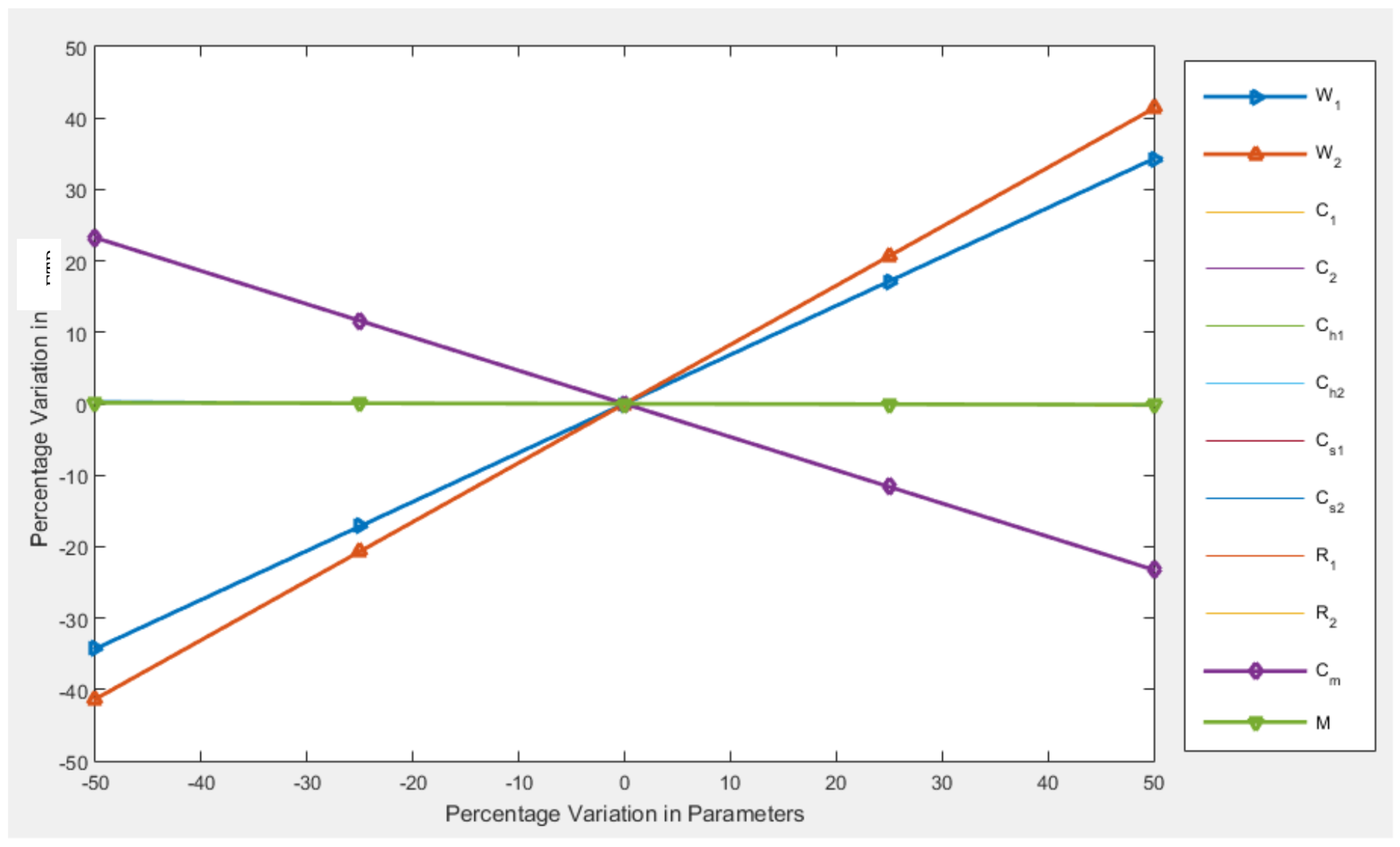
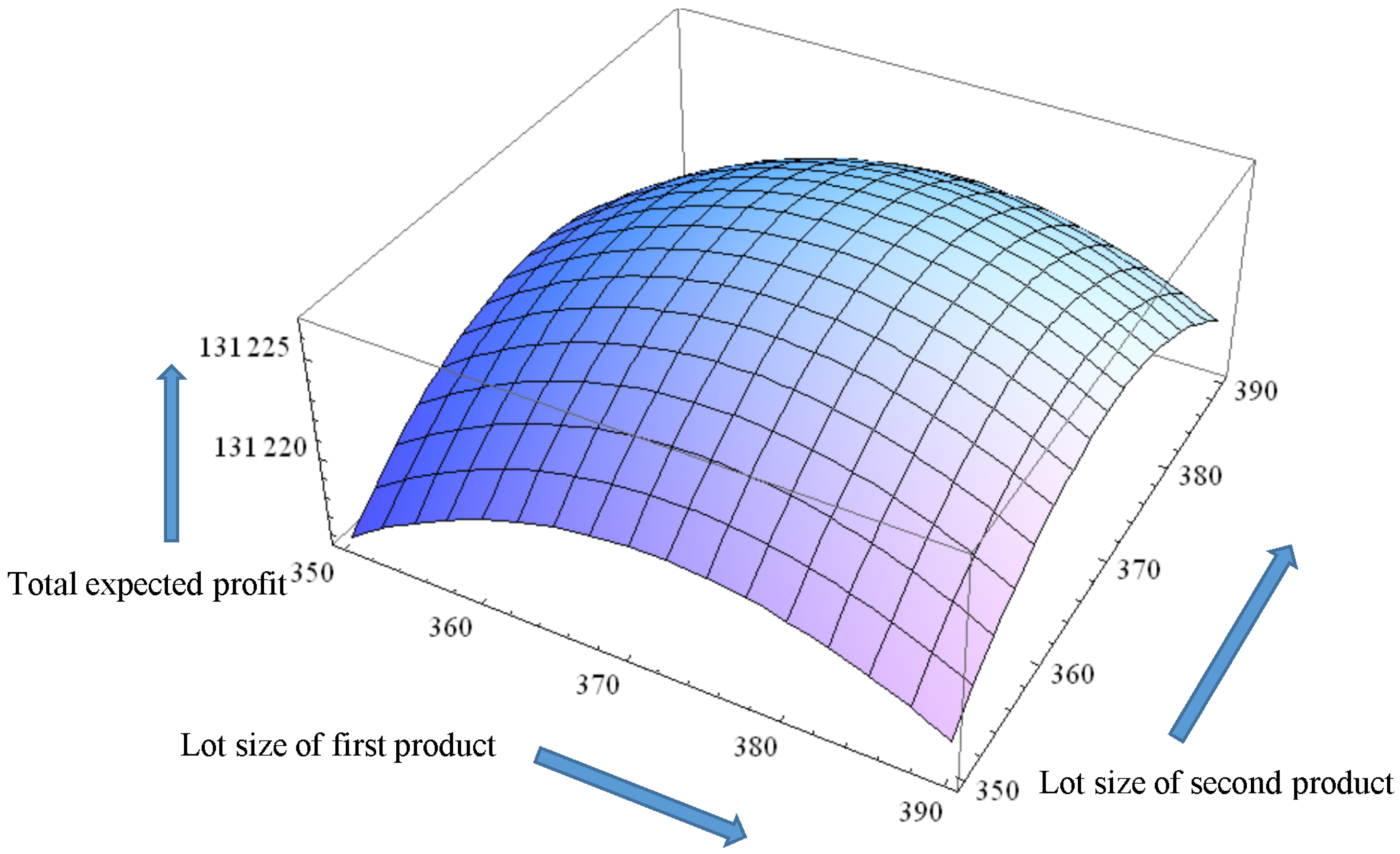
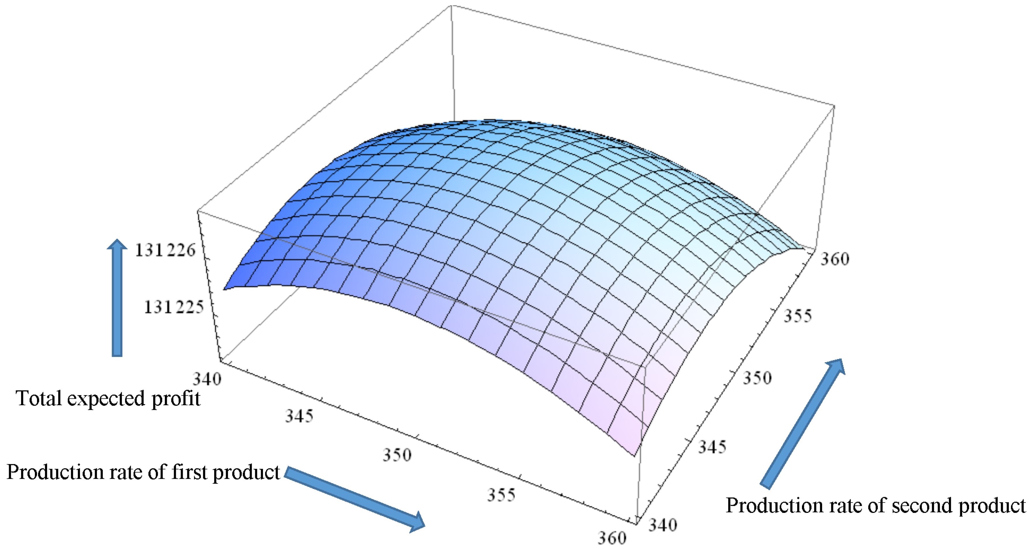
The model is tested through numerical experiments and the global optimality is tested at the optimal points.

5. Numerical Experiment

This section consists of numerical examples and sensitivity of the model.

5.1. Numerical Examples

There are two examples in this section.

5.2. Example 1

The following parametric values are taken from [2] as in

Table 2. The optimal values of Example 1.

i	${\mathit{D}}_{\mathit{i}}$ units	${\mathit{W}}_{\mathit{i}}$ $/unit	${\mathit{C}}_{\mathit{i}}$ $/unit	${\mathit{C}}_{{\mathit{h}}_{\mathit{i}}}$ $/unit/year	${\mathit{C}}_{{\mathit{s}}_{\mathit{i}}}$ $/setup	${\mathit{R}}_{\mathit{i}}$ $/unit	${\mathit{\xi }}_{\mathit{i}}$ sq. feet/unit	${\mathit{\varphi }}_{\mathit{i}}$ $/unit
1	300	300	2.7	1.8	920	95	5	10
2	310	350	1.8	2.1	1000	102	4	12
i	${\mathit{C}}_{{\mathit{s}}_{\mathit{i}}}^{{}^{\prime }}$$/setup	${\mathit{C}}_{{\mathit{h}}_{\mathit{i}}}^{{}^{\prime }}$$/unit/year	${\mathit{C}}_{\mathit{i}}^{{}^{\prime }}$$/unit	${\mathit{R}}_{\mathit{i}}^{{}^{\prime }}$$/unit
1	80	0.2	0.3	5
2	100	0.4	0.2	8
$\mathit{M}$$/unit	${\mathit{C}}_{\mathit{m}}$$/unit	$\mathit{X}$$	$\mathit{A}$sq.feet	$\mathit{B}$$	$\mathit{r}$	$\mathit{\alpha }$	$\mathit{\beta }$	$\mathit{\gamma }$	$\mathit{\delta }$
200	100	30	10,000	15,000	0.90	0.05	0.25	2	0.70

. The model considers for the Example 1 with two items. Figure 3, Figure 4, Figure 5, Figure 6, Figure 7 and Figure 8 indicate the variation in development cost with failure rate, variation in expected total profit per unit time with other cost key parameters, expected total profit versus lot size of two products, expected total profit versus production rate of two products, expected total profit versus lot size of first product and failure rate, and expected total profit versus production rate of 1st product and failure rate, respectively.

The results of Example 1 are given in

Table 3. The optimal values of Example 1.

${\mathit{ETP}}^{*}$$\$/$year	${\mathit{Q}}_1^{*}$ units	${\mathit{Q}}_2^{*}$ units	${\mathit{P}}_1^{*}$ unit/year	${\mathit{P}}_2^{*}$ unit/year	${\mathit{\eta }}^{*}$
131,219	371.64	341.91	349.05	279.99	0.43

.

5.3. Example 2

For Example 2, the model considers three items. The following parametric values are taken from Sana (2010b) as in

Table 4. Input parameters for $i=3$.

i	${\mathit{D}}_{\mathit{i}}$ units	${\mathit{W}}_{\mathit{i}}$ $/unit	${\mathit{C}}_{\mathit{i}}$ $/unit	${\mathit{C}}_{{\mathit{h}}_{\mathit{i}}}$ $/unit/year	${\mathit{C}}_{{\mathit{s}}_{\mathit{i}}}$ $/setup	${\mathit{R}}_{\mathit{i}}$ $/unit	${\mathit{\xi }}_{\mathit{i}}$ sq. feet/unit	${\mathit{\varphi }}_{\mathit{i}}$ $/unit
1	300	300	2.7	1.8	920	95	5	10
2	310	350	1.8	2.1	1000	102	4	12
3	330	400	3.6	2.5	1050	120	6	14
i	${\mathit{C}}_{{\mathit{s}}_{\mathit{i}}}^{{}^{\prime }}$$/setup	${\mathit{C}}_{{\mathit{h}}_{\mathit{i}}}^{{}^{\prime }}$$/unit/year	${\mathit{C}}_{\mathit{i}}^{{}^{\prime }}$$/unit	${\mathit{R}}_{\mathit{i}}^{{}^{\prime }}$$/unit
1	80	0.2	0.3	5
2	100	0.4	0.2	8
3	150	0.5	0.4	10
$\mathit{M}$$/unit	${\mathit{C}}_{\mathit{m}}$$/unit	$\mathit{X}$$	$\mathit{A}$sq.feet	$\mathit{B}$$	$\mathit{r}$	$\mathit{\alpha }$	$\mathit{\beta }$	$\mathit{\gamma }$	$\mathit{\delta }$
200	100	30	10,000	15,000	0.90	0.05	0.25	2	0.70

. The model considers for Example 2 with three items.

The results of Example 2 are given in

Table 5. The optimal values of Example 2.

${\mathit{ETP}}^{*}$$\$/$year	${\mathit{Q}}_1^{*}$ units	${\mathit{Q}}_2^{*}$ units	${\mathit{Q}}_3^{*}$ units	${\mathit{P}}_1^{*}$ unit/year	${\mathit{P}}_2^{*}$ unit/year	${\mathit{P}}_3^{*}$ unit/year	${\mathit{\eta }}^{*}$
226,158	372.69	372.39	372.19	349.11	347.19	355.16	0.43

.

5.4. Sensitivity Analysis

The sensitivity analysis of key parameters are considered and major findings can be concluded from the sensitivity analysis

Table 6. Sensitivity analysis of key parameters.

Parameters	Changes (in %)	ETP (%)	Parameters	Changes (in %)	ETP (%)
$W_1$	−50%	−34.29	$C_{s1}$	−50%	+0.36
	−25%	−17.15		−25%	+0.16
	+25%	+17.15		+25%	−0.15
	+50%	+34.29		+50%	−0.28
$W_2$	−50%	−41.34	$C_{s2}$	−50%	+0.40
	−25%	−20.67		−25%	+0.19
	+25%	+20.67		+25%	−0.17
	+50%	+41.34		+50%	−0.32
$C_1$	−50%	+0.34	$R_1$	−50%	+0.14
	−25%	+0.17		−25%	+0.06
	+25%	−0.17		+25%	−0.04
	+50%	−0.34		+50%	−0.08
$C_2$	−50%	+0.24	$R_2$	−50%	+0.16
	−25%	+0.12		−25%	+0.07
	+25%	−0.12		+25%	−0.05
	+50%	−0.24		+50%	−0.09
$C_{h1}$	−50%	+0.03	$M$	−50%	+0.14
	−25%	+0.01		−25%	+0.07
	+25%	−0.007		+25%	−0.07
	+50%	−0.01		+50%	−0.13
$C_{h2}$	−50%	+0.03	$C_m$	−50%	+23.24
	−25%	+0.01		−25%	+11.62
	+25%	−0.006		+25%	−11.62
	+50%	−0.006		+50%	−23.24

.

Table 6 is showing the effect of changes by certain percentage (−50%, −25%, +25%, +50%) of the key parameters and selling-price on the optimal values of total expected profit.

The following are some inferences from obtained results:

• The higher the selling-price, the higher the optimal value of the profit and vice versa. It is generally true that, keeping all costs the same, and an increase in selling-price increases the profit. However, in specific cases, where demand depends upon the selling-price, there could be an optimal point beyond which, if selling-price is increased, the demand and hence profit could decrease. As demand is not price-dependent in the considered model, profit can thus be increased by increasing product selling-price.
• On the other hand, the increase in inspection cost decreases the optimal value of the profit. Some industries do not consider inspection as a value added process to the final product, thus the investment in inspection does not give value apparently. Investing more for inspection results in losing profit. Likewise, reworking cost is another such type of cost that is considered non-value added to the final product because the investment is being done again to make the product saleable. Reworking cost also affects the profit in the same way as the inspection cost does.
• Observing the data in Table 6, it can be concluded generally that variation in holding cost has a less significant effect on the optimal profit of the system. However, if it is the reverse, but there is very little variation in the profit. The results are justified because holding cost is very small as compared to other costs for this model as products are not holding for a long-time. Similarly, variation in setup cost has a nominal effect on optimality of profit.
• Variation in material cost varies the optimal value of total profit significantly as it is obvious from Table 6. In a production system, the major costs are incurred by material and production. Working on these areas, it can reduce the total cost to a considerable amount and hence it can increase the profit.
• Effect of fixed cost changes are the reverse for the optimal value of the total expected profit, whereas the effect is very nominal.
• It can be summarized that the optimal profit value is highly sensitive to the selling-price and material cost, while there are nominal changes in optimal profit for the changes in other parameters. From a managerial point of view, concerned with the total amount of profit, the optimal selling-price and material cost are the most important factors to control its optimal value.

5.5. Managerial Insights

Some recommendations are given for the industry as follows:

• The major insight for the industry manager is that they have smart production systems without having the information about the benefit of energy consumption calculation. Basically, for a smart production system, a portion of the total amount of labor is replaced by some smart machines as results, the consumption of energy increases. However, no research has considered the multi-item smart production with energy consumption and random failure rate yet. Thus, the result of this study would support the smart industry manager for obtaining more profit.
• As the study is considered for a smart production system, the random breakdown time is still considered. Thus, the smart industry manager can easily calculate the due date for any delivery based on the available data for the random breakdown time. They might get support if they have any issues for budget and space.
• The smart managers always obtain the profit at the optimum values of the decision variables. They can obtain the information easily about the cost for the energy sector how much energy can be used for which sector. They can decide on the amount of optimized energy consumption level or not. If they found that the energy cost is getting high, they can consider the replacement of this energy consumption with any other renewable energy. This can benefit for the random defective rate information during long-run smart production systems.

6. Conclusions

This study extended a basic production model with some realistic assumptions explained here.

• The inspection cost for multi-stage smart production systems with smart machines under energy consumption is not negligible.
• The development cost is not constant for any multi-stage smart production system. This study considered that the development cost was dependent on the labor cost, energy resource cost and the failure rate of the smart production system.
• A multi-item smart production system without budget and space constraints is almost impossible. Thus, this model considered a space and a budget constraint to match with reality.
• The energy consideration in multi-item smart production systems had not yet been considered by authors. This study introduced the consideration of energy in a smart production systems under budget and space constraints for the first time.

It was considered that system reliability depends upon system failure rate and the system reliability was considered as a system design variable. The greater the investment, the more reliable the the system would be. Investment for the system reliability was done for production costs that are composed of development costs, material costs and tool/die costs. Production of defective items was dependent upon the state of systems, when it was moved from in-control state to out-of-control state and the movement time was supposed as random, which followed an exponential distribution, and an expected number of defective items was calculated during the production cycle under energy consideration. The mathematical model for expected total profit was formulated and solved using the Kuhn–Tucker method considering system constraints. To show the practical implications of the model, numerical examples have been solved to compute the optimal value of the objective function and that of decision variables. Finally, sensitivity analysis was presented to study the effect of different system parameters on the optimal value of decision variables and that of objective function. The industry manager obtained the benefit of having information of the energy consumption from all workstations of multi-item smart production systems. They obtained the expected schedule of due dates as they had the information about random defective rates even though smart machines were used. The main limitation of the model is that the demand is known as constant, which may be random or uncertain based on the real-life situation. The smart production system is considered, but autonomation policy is not adopted under the effect of energy. The labor cost is incorporated, but the quality of labor i.e., skilled, semi-skilled, or unskilled is not considered. Those are the main limitations in the direction of energy, which can be considered for further study of this research model. The model can be extended by considering the concept of [15] as imperfect inspection and non-inspected products with warranty. The preventive and corrective maintenance can be another major extension of the model considering planned backorder. This model can be extended further (see, for reference, [1]).

References

1. Cárdenas-Barrón, L.E. Economic production quantity with rework process at a single-stage manufacturing system with planned backorders. Comput. Ind. Eng. 2009, 57, 1105–1113. [Google Scholar] [CrossRef]
2. Sana, S.S. A production-inventory model in an imperfect production process. Eur. J. Oper. Res. 2010, 200, 451–464. [Google Scholar] [CrossRef]
3. Kim, C.H.; Hong, Y. An optimal production run length in deteriorating production processes. Int. J. Prod. Econ. 1999, 58, 183–189. [Google Scholar] [CrossRef]
4. Rosenblatt, M.J.; Lee, H.L. Economic production cycles with imperfect production processes. IIE Trans. 1986, 18, 48–55. [Google Scholar] [CrossRef]
5. Giri, B.; Dohi, T. Exact formulation of stochastic EMQ model for an unreliable production system. J. Oper. Res. Soc. 2005, 56, 563–575. [Google Scholar] [CrossRef]
6. Sana, S.S.; Goyal, S.K.; Chaudhuri, K. An imperfect production process in a volume flexible inventory model. Int. J. Prod. Econ. 2007, 105, 548–559. [Google Scholar] [CrossRef]
7. Chiu, Y.-S.P.; Chen, K.-K.; Cheng, F.-T.; Wu, M.-F. Optimization of the finite production rate model with scrap, rework and stochastic machine breakdown. Comput. Math. Appl. 2010, 59, 919–932. [Google Scholar] [CrossRef]
8. González, H.; Calleja, A.; Pereira, O.; Ortega, N.; López de Lacalle, L.N.; Barton, M. Super abrasive machining of integral rotary components using grinding flank tools. Metals 2018, 8, 24. [Google Scholar] [CrossRef]
9. Egea, A.J.S.; Deferrari, N.; Abate, G.; Martínez Krahmer, D.; López de Lacalle, L.N. Short-cut method to assess a gross available energy in a medium-load screw friction press. Metals 2018, 8, 173. [Google Scholar] [CrossRef]
10. Sarkar, B. An EOQ model with delay in payments and stock dependent demand in the presence of imperfect production. Appl. Math. Comput. 2012, 218, 8295–8308. [Google Scholar] [CrossRef]
11. Sarkar, B. An EOQ model with delay in payments and time varying deterioration rate. Math. Comput. Model. 2012, 55, 367–377. [Google Scholar] [CrossRef]
12. Sarkar, B. An inventory model with reliability in an imperfect production process. Appl. Math. Comput. 2012, 218, 4881–4891. [Google Scholar] [CrossRef]
13. Chakraborty, T.; Giri, B. Lot sizing in a deteriorating production system under inspections, imperfect maintenance and reworks. Oper. Res. 2014, 14, 29–50. [Google Scholar] [CrossRef]
14. Sarkar, B.; Cárdenas-Barrón, L.E.; Sarkar, M.; Singgih, M.L. An economic production quantity model with random defective rate, rework process and backorders for a single stage production system. J. Manuf. Syst. 2014, 33, 423–435. [Google Scholar] [CrossRef]
15. Sarkar, B.; Saren, S. Product inspection policy for an imperfect production system with inspection errors and warranty cost. Eur. J. Oper. Res. 2016, 248, 263–271. [Google Scholar] [CrossRef]
16. Pasandideh, S.H.R.; Niaki, S.T.A.; Nobil, A.H.; Cárdenas-Barrón, L.E. A multi-product single machine economic production quantity model for an imperfect production system under warehouse construction cost. Int. J. Prod. Econ. 2015, 169, 203–214. [Google Scholar] [CrossRef]
17. Purohit, A.K.; Shankar, R.; Dey, P.K.; Choudhary, A. Non-stationary stochastic inventory lot-sizing with emission and service level constraints in a carbon cap-and-trade system. J. Clean. Prod. 2016, 113, 654–661. [Google Scholar] [CrossRef] [Green Version]
18. Sana, S.S. An economic production lot size model in an imperfect production system. Eur. J. Oper. Res. 2010, 201, 158–170. [Google Scholar] [CrossRef]
19. Cárdenas-Barrón, L.E.; Chung, K.-J.; Kazemi, N.; Shekarian, E. Optimal inventory system with two backlog costs in response to a discount offer: Corrections and complements. Oper. Res. 2018, 18, 97–104. [Google Scholar] [CrossRef]
20. Tiwari, S.; Jaggi, C.K.; Gupta, M.; Cárdenas-Barrón, L.E. Optimal pricing and lot-sizing policy for supply chain system with deteriorating items under limited storage capacity. Int. J. Prod. Econ. 2018, 200, 278–290. [Google Scholar] [CrossRef]
21. Tiwari, S.; Cárdenas-Barrón, L.E.; Goh, M.; Shaikh, A.A. Joint pricing and inventory model for deteriorating items with expiration dates and partial backlogging under two-level partial trade credits in supply chain. Int. J. Prod. Econ. 2018, 200, 16–36. [Google Scholar] [CrossRef]
22. Huang, Y.-F.; Lai, C.-S.; Shyu, M.-L. Retailer’s EOQ model with limited storage space under partially permissible delay in payments. Math. Prob. Eng. 2007, 2007, 90873. [Google Scholar] [CrossRef]
23. Pasandideh, S.H.R.; Niaki, S.T.A. A genetic algorithm approach to optimize a multi-products EPQ model with discrete delivery orders and constrained space. Appl. Math. Comput. 2008, 195, 506–514. [Google Scholar] [CrossRef]
24. Hafshejani, K.F.; Valmohammadi, C.; Khakpoor, A. Retracted: Using genetic algorithm approach to solve a multi-product EPQ model with defective items, rework, and constrained space. J. Ind. Eng. Int. 2012, 8, 1–8. [Google Scholar] [CrossRef]
25. Mahapatra, G.; Mandal, T.; Samanta, G. An EPQ model with imprecise space constraint based on intuitionists fuzzy optimization technique. J. Mult.-Valued Log. Soft Comput. 2012, 19, 409–423. [Google Scholar] [CrossRef]
26. Mohan, S.; Mohan, G.; Chandrasekhar, A. Multi-item, economic order quantity model with permissible delay in payments and a budget constraint. Eur. J. Ind. Eng. 2008, 2, 446–460. [Google Scholar] [CrossRef]
27. Hou, K.-L.; Lin, L.-C. Investing in setup reduction in the EOQ model with random yields under a limited capital budget. J. Inf. Optim. Sci. 2011, 32, 75–83. [Google Scholar] [CrossRef]
28. Taleizadeh, A.; Jalali-Naini, S.G.; Wee, H.-M.; Kuo, T.-C. An imperfect multi-product production system with rework. Sci. Iran. 2013, 20, 811–823. [Google Scholar] [CrossRef]
29. Cárdenas-Barrón, L.E.; Treviño-Garza, G.; Widyadana, G.A.; Wee, H.-M. A constrained multi-products EPQ inventory model with discrete delivery order and lot size. Appl. Math. Comput. 2014, 230, 359–370. [Google Scholar] [CrossRef]
30. Du, Y.; Hu, G.; Xiang, S.; Zhang, K.; Liu, H.; Guo, F. Estimation of the diesel particulate filter soot load based on an equivalent circuit model. Energies 2018, 11, 472. [Google Scholar] [CrossRef]
31. Todde, G.; Murgia, L.; Caria, M.; Pazzona, A. A comprehensive energy analysis and related carbon footprint of dairy farms, Part 2: Investigation and modeling of indirect energy requirements. Energies 2018, 11, 463. [Google Scholar] [CrossRef]
32. Tomić, T.; Schneider, D.R. The role of energy from waste in circular economy and closing the loop concept-Energy analysis approach. Renew. Sustain. Energy Rev. 2018, 98, 268–287. [Google Scholar] [CrossRef]
33. Haraldsson, J.; Johansson, M.T. Review of measures for improved energy efficiency in production-related processes in the aluminium industry-from electrolysis to recycling. Renew. Sustain. Energy Rev. 2018, 93, 525–548. [Google Scholar] [CrossRef]
34. Xua, L.; Cheng, J.-H.; Liu, P.; Wang, Q.; Xu, Z.-X.; Liu, Q.; Shen, J.-Y.; Wang, L.-J. Production of bio-fuel oil from pyrolysis of plant acidified oil. Renew. Energy 2019, 130, 910–919. [Google Scholar] [CrossRef]
Figure 1. Process flow for multi-product production system
Energies 11 02958 g001
Figure 2. Economic production quantity model for multi-product systems.
Energies 11 02958 g002
Figure 3. Variation in development cost C 1 ( η ) with varying system failure rate ( η ).
Energies 11 02958 g003
Figure 4. Variation in expected total profit per unit time (ETP) with variation in system parameters (selling price of first product w 1 , selling price of second product w 2 , inspection cost of first product C 1 , inspection cost of second product C 2 , holding of first product C h 1 , holding of second product C h 2 , setup cost of first product C s 1 , setup cost of second product C s 2 , rework cost of first product R 1 , rework cost of second product R 2 , material cost C m , and fixed cost M).
Energies 11 02958 g004
Figure 5. Expected total profit (ETP) versus lot size of two products ( Q 1 , Q 2 ).
Energies 11 02958 g005
Figure 6. Expected total profit (ETP) versus production rate of two products ( P 1 , P 2 ).
Energies 11 02958 g006
Figure 7. Expected total profit (ETP) versus lot size of first product Q 1 and failure rate η .
Energies 11 02958 g007
Figure 8. Expected total profit (ETP) versus production rate P 1 of 1st product and failure rate η .
Energies 11 02958 g008