Hybrid Imperialist Competitive and Grey Wolf Algorithm to Solve Multiobjective Optimal Power Flow with Wind and Solar Units


Abstract
1. Introduction
2. OPF Problem Formulation
2.1. Objective Functions
2.1.1. Wind Cost Function
- and symbolizes speed and rated speed of WE generators,
- and symbolizes cut-in and cut-out speed of WE generators,
- , symbolizes shape and scale parameters of the Weibull distribution.
2.1.2. PV Cost Function
- Solar cells or PV cells are hypersensitive to the amount of solar radiation. The PDF of solar radiation can be modeled by a beta distribution [12]:where is the gamma function, and are parameters of the beta distribution, and R is the solar radiation.
- The relation between power output of PV and output power of solar cell generator which is related to the solar radiation can be calculated as follows:where and are solar radiation in W/m2. Usually, a typical solar radiation point is set to 150 W/m2, and it is set to 100 W/m2 under standard conditions.
2.1.3. Basic Fuel Cost Function
2.1.4. Piecewise Quadratic Fuel Cost Function
2.1.5. Piecewise Quadratic Fuel Cost with Valve Point Loading
2.1.6. Emission Cost Function
2.1.7. Power Loss Cost Function
2.1.8. Fuel Cost and Active Power Loss Cost Function
2.1.9. Fuel Cost and Voltage Deviation
2.1.10. Fuel Cost and Voltage Stability Enhancement
2.1.11. Fuel Cost and Voltage Stability Enhancement during Contingency Condition
2.1.12. Fuel Cost, Emission, Voltage Deviation, and Active Power Loss
2.2. Constraints
3. New Hybrid Optimization Algorithm
3.1. Imperialist Competitive Algorithm (ICA)
3.1.1. Creation of Initial Empires
3.1.2. Assimilation
3.1.3. Revolution
3.1.4. Exchanging Positions of a Colony and the Imperialist
3.1.5. Union of Empires
3.1.6. Total Empire Power
3.1.7. Imperialistic Competition
3.2. Grey Wolf Optimizer (GWO)
3.2.1. Social Hierarchy
3.2.2. Encircling Prey
3.2.3. Hunting
3.2.4. Attacking Prey (Exploitation)
3.2.5. Search for Prey (Exploration)
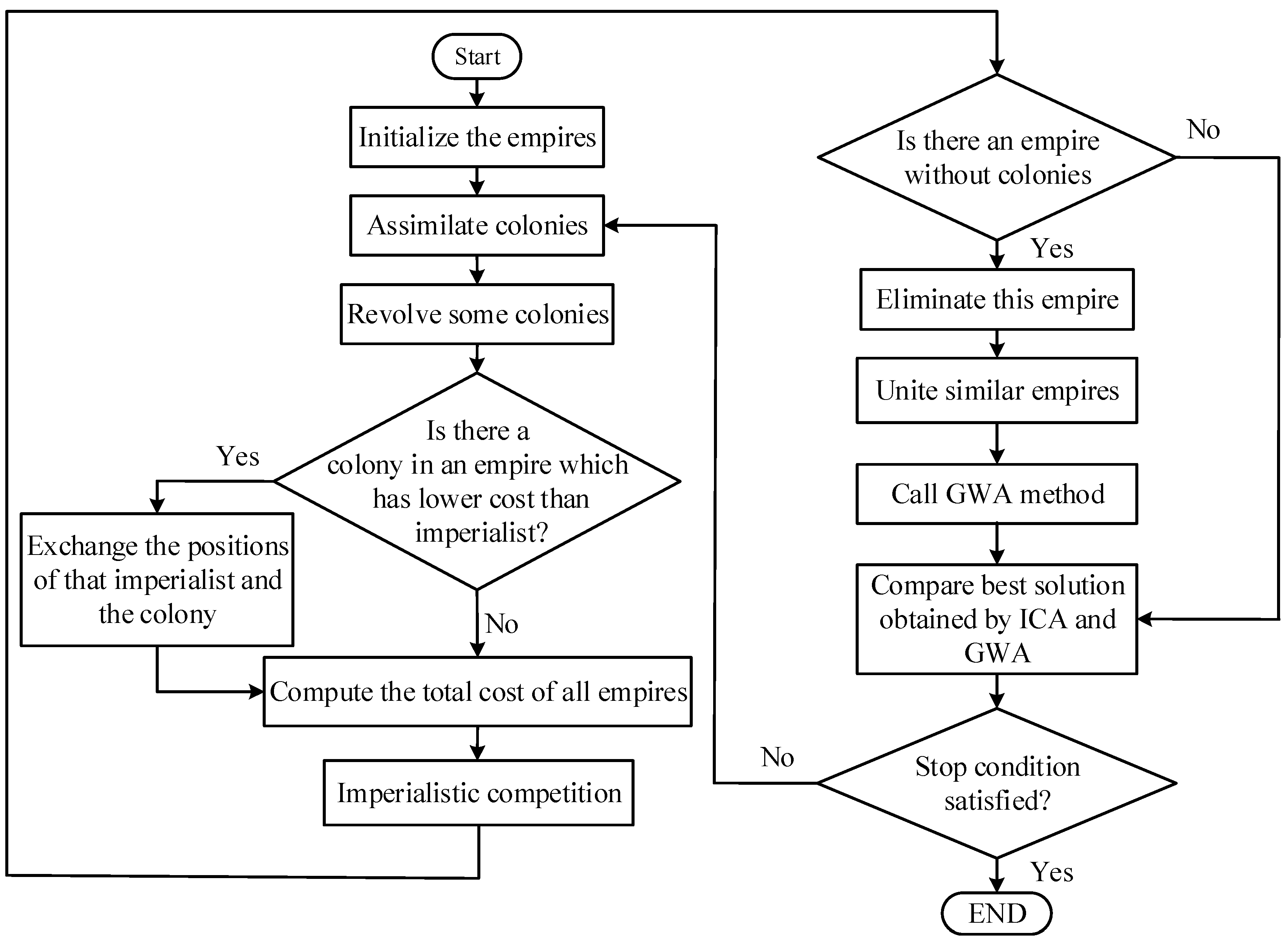
3.3. Hybrid IC-GWA Optimization Approach
- The power system data is specified. The HIC-GWA parameters are determined.
- Initialize the countries randomly, calculate their costs, and use assimilation.
- Revolution.
- Exchange positions between imperialist and colony if it has a lower cost.
- Unite similar empires.
- Calculate the total cost of all empires.
- Imperialist competition.
- Discard powerless empires.
- Use solution obtained by ICA as initial condition for GWA.
- The lower solution between ICA and GWA is saved as best solution.
- Go to step (ii) if the stop condition is not satisfied, otherwise, finish simulation.
4. Simulation Results
4.1. IEEE 30 Bus Test System
4.1.1. Simple Objective OPF
4.1.2. Multiobjective OPF
4.2. The IEEE 118 Bus Power System
4.3. HIC-GWA Robustness Analysis
5. Conclusions
Author Contributions
Funding
Conflicts of Interest
Nomenclature
| direct cost of WE and PV($/h) | |
| underestimating penalty cost of ith WE and PV ($/h) | |
| overestimating penalty cost of ith WE and PV ($/h) | |
| total cost of ith WE and PV ($/h) | |
| direct cost coefficient of WE and PV ($/MW) | |
| underestimating coefficient cost of ith WE and PV ($/MW) | |
| overestimating coefficients cost of ithWE and PV ($/MW) | |
| power of the ith WE (MW) | |
| power of the ith PV (MW) | |
| rated power of the ith WE (MW) | |
| rated power of the ith PV(MW) | |
| number of WEs | |
| number of PVs |
References
- Carpentier, J. Optimal power flows. Int. J. Elect. Power Energy Syst. 1979, 1, 3–15. [Google Scholar] [CrossRef]
- Momoh, J.A.; Koessler, R.J.; Bond, M.S.; Stott, B.; Sun, D.; Papalexopoulos, A.; Ristanovic, P. Challenges to optimal power flow. IEEE Trans. Power Syst. 1997, 12, 444–447. [Google Scholar] [CrossRef]
- Capitanescu, F.; Martinez Ramos, J.L.; Panciatici, P.; Kirschen, D.; Platbrood, L.; Wehenkel, L. State-of-the-art challenges and future trends in security constrained optimal power flow. Elect. Power Syst. Res. 2011, 81, 1731–1741. [Google Scholar] [CrossRef]
- Low, S.H. Convex Relaxation of Optimal Power Flow: Parts I & II. IEEE Trans. Control Netw. Syst. 2014, 1, 15–27. [Google Scholar]
- Panciatici, P.; Campi, M.; Garatti, S.; Low, S.; Molzahn, D.; Sun, A.; Wehenkel, L. Advanced optimization methods for power systems. In Proceedings of the 18th Power Systems Computation Conference (PSCC), Wroclaw, Poland, 18–22 August 2014; pp. 1–18. [Google Scholar]
- Cain, M.B.; O’Neill, R.P.; Castillo, A. History of Optimal Power Flow and Formulations. Available online: https://www.ferc.gov/industries/electric/indus-act/market-planning/opf-papers/acopf-1-history-formulation-testing.pdf (accessed on 18 June 2018).
- Molzahn, D.K.; Dorfler, F.; Sandberg, H.; Low, S.H.; Chakrabarti, S.; Baldick, R.; Lavaei, J. A survey of distributed optimization and control algorithms for electric power systems. IEEE Trans. Smart Grid 2017, 8, 2941–2962. [Google Scholar] [CrossRef]
- Frank, S.; Steponavice, I.; Rebennack, S. Optimal power flow: A bibliographic survey parts I and II. Energy Syst. 2012, 3, 221–289. [Google Scholar] [CrossRef]
- Baydar, B.; Gozde, H.; Taplamacioglu, M.C.; Kucuk, A.O. Resilient Optimal Power Flow with Evolutionary Computation Methods: Short Survey. In Power Systems Resilience; Mahdavi, T.N., Ed.; Springer: Cham, Switzerland, 2019. [Google Scholar]
- Thomson, M.; Infield, D. Network power-flow analysis for a high penetration of distributed generation. IEEE Trans. Power Syst. 2007, 22, 1157–1162. [Google Scholar] [CrossRef]
- Bonface, O.N.; Hideharu, S.; Tsuyoshi, F. Optimal power flow considering line-conductor temperature limits under high penetration of intermittent renewable energy sources. Int. J. Electr. Power Energy Syst. 2018, 101, 255–267. [Google Scholar]
- Morshed, M.J.; Ben Hmida, J.; Fekih, A. A probabilistic multiobjective approach for power flow optimization in hybrid wind-PV-PEV systems. Appl. Energy 2018, 211, 1136–1149. [Google Scholar] [CrossRef]
- Pourakbari-Kasmaei, M.; Sanches, J.R. Logically constrained optimal power flow: Solver-based mixed-integer nonlinear programming model. Int. J. Electr. Power Energy Syst. 2018, 97, 240–249. [Google Scholar] [CrossRef]
- Momoh, J.A.; Adapa, R.; El-Hawary, M.E. A review of selected optimal power flow literature to 1993. I. Nonlinear and quadratic programming approaches. IEEE Trans. Power Syst. 1999, 14, 96–104. [Google Scholar] [CrossRef]
- Momoh, J.A.; El-Hawary, M.E.; Adapa, R. A review of selected optimal power flow literature to 1993. II. Newton linear programming and interior point methods. IEEE Trans. Power Syst. 1999, 14, 105–111. [Google Scholar] [CrossRef]
- Ghasemi, M.; Ghavidel, S.; Akbari, E.; Vahed, A.A. Solving non-linear, non-smooth and non-convex optimal power flow problems using chaotic invasive weed optimization algorithms based on chaos. Energy 2014, 73, 340–353. [Google Scholar] [CrossRef]
- Ghasemi, M.; Ghavidel, S.; Aghaei, J.; Gitizadeh, M.; Falah, H. Application of chaos-based chaotic invasive weed optimization techniques for environmental OPF problems in the power system. Chaos Solitons Fractals 2014, 69, 271–284. [Google Scholar] [CrossRef]
- Boussaïd, I.; Lepagnot, J.; Siarry, P. A survey on optimization metaheuristics. Inf. Sci. 2013, 237, 82–117. [Google Scholar] [CrossRef]
- Mohamed, A.A.; Mohamed, Y.S.; El-Gaafary, A.A.M.; Hemeida, A.M. Optimal power flow using moth swarm algorithm. Electr. Power Syst. Res. 2017, 142, 190–206. [Google Scholar] [CrossRef]
- Karami, A. A fuzzy anomaly detection system based on hybrid pso-k means algorithm in content-centric networks. Neurocomputing 2015, 149, 1253–1269. [Google Scholar] [CrossRef]
- Dos Santos Coelho, L.; Mariani, V.C.; Leite, J.V. Solution of Jiles-Atherton vector hysteresis parameters estimation by modified Differential Evolution approaches. Expert Syst. Appl. 2012, 39, 2021–2025. [Google Scholar] [CrossRef]
- Mirjalili, S. Moth-flame optimization algorithm: A novel nature-inspired heuristic paradigm. Knowl. Based Syst. 2015, 89, 228–249. [Google Scholar] [CrossRef]
- Yang, X.S. Flower Pollination Algorithm for Global Optimization. In Unconventional Computation and Natural Computation; Springer: Berlin, Germany, 2012; pp. 240–249. [Google Scholar]
- Kumar, A.R.; Premalatha, L. Optimal power flow for a deregulated power system using adaptive real coded biogeography-based optimization. Int. J. Electr. Power Energy Syst. 2015, 73, 393–399. [Google Scholar] [CrossRef]
- El-Fergany, A.A.; Hasanien, H.M. Single and multiobjective optimal power flow using grey wolf optimizer and differential evolution algorithms. Electr. Power Compon. Syst. 2015, 43, 1548–1559. [Google Scholar] [CrossRef]
- Ghasemi, M.; Ghavidel, S.; Ghanbarian, M.M.; Gitizadeh, M. Multiobjective optimal electric power planning in the power system using Gaussian bare-bones imperialist competitive algorithm. Inf. Sci. 2015, 294, 286–304. [Google Scholar] [CrossRef]
- Adaryani, M.R.; Karami, A. Artificial bee colony algorithm for solving multiobjective optimal power flow problem. Int. J. Electr. Power Energy Syst. 2013, 53, 219–230. [Google Scholar] [CrossRef]
- Niknam, T.; Narimani, M.R.; Azizipanah, A.R. A new hybrid algorithm for optimal power flow considering prohibited zones and valve point effect. Energy Convers. Manag. 2012, 58, 197–206. [Google Scholar] [CrossRef]
- Ghasemi, M.; Ghavidel, S.; Gitizadeh, M.; Akbari, E. An improved teaching-learning-based optimization algorithm using Lévy mutation strategy for non-smooth optimal power flow. Int. J. Electr. Power Energy Syst. 2015, 65, 375–384. [Google Scholar] [CrossRef]
- Bouchekara, H.; Abido, M.A.; Boucherma, M. Optimal power flow using teaching-learning-based optimization technique. Electr. Power Syst. Res. 2014, 114, 49–59. [Google Scholar] [CrossRef]
- Narimani, M.R.; Azizipanah, A.R.; Zoghdar, M.S.B.; Gholami, K. A novel approach to multiobjective optimal power flow by a new hybrid optimization algorithm considering generator constraints and multi-fuel type. Energy 2013, 49, 119–136. [Google Scholar] [CrossRef]
- Roy, R.; Jadhav, H.T. Optimal power flow solution of power system incorporating stochastic wind power using Gbest guided artificial bee colony algorithm. Int. J. Electr. Power Energy Syst. 2015, 64, 562–578. [Google Scholar] [CrossRef]
- Abaci, K.; Yamacli, V. Differential search algorithm for solving multiobjective optimal power flow problem. Int. J. Electr. Power Energy Syst. 2016, 79, 1–10. [Google Scholar] [CrossRef]
- Reddy, S.S.; Bijwe, P.R.; Abhyankar, A.R. Faster evolutionary algorithm based optimal power flow using incremental variables. Int. J. Electr. Power Energy Syst. 2014, 54, 198–210. [Google Scholar] [CrossRef]
- Singh, R.P.; Mukherjee, V.; Ghoshal, S.P. Particle swarm optimization with an aging leader and challenger’s algorithm for the solution of optimal power flow problem. Appl. Soft Comput. 2016, 40, 161–177. [Google Scholar] [CrossRef]
- Coello Coello, C.A. A Comprehensive Survey of Evolutionary-Based Multiobjective Optimization Techniques. Knowl. Inf. Syst. 1999, 1, 269–308. [Google Scholar] [CrossRef]
- Khabbazi, A.; Atashpaz, G.E.; Lucas, C. Imperialist competitive algorithm for minimum bit error rate beamforming. Int. J. Bio-Inspired Comput. 2009, 1, 125–133. [Google Scholar] [CrossRef]
- Kaveh, A. Imperialist Competitive Algorithm. In Advances in Metaheuristic Algorithms for Optimal Design of Structures; Springer: Cham, Switzerland, 2017. [Google Scholar]
- Ardalan, A.; Karimi, S.; Poursabzi, O.; Naderi, B. A novel imperialist competitive algorithm for generalized traveling salesman problems. Appl. Soft Comput. 2015, 26, 546–555. [Google Scholar] [CrossRef]
- Mirjalili, S.; Mirjalili, S.M.; Lewis, A. Grey wolf optimizer. Adv. Eng. Softw. 2014, 69, 46–61. [Google Scholar] [CrossRef]
- Zhang, X.; Miao, Q.; Liu, Z.; He, Z. An adaptive stochastic resonance method based on grey wolf optimizer algorithm and its application to machinery fault diagnosis. ISA Trans. 2017, 71, 206–214. [Google Scholar] [CrossRef] [PubMed]
- Hooshmand, R.A.; Morshed, M.J.; Parastegari, M. Congestion management by determining optimal location of series FACTS devices using hybrid bacterial foraging and Nelder-Mead algorithm. Appl. Soft Comput. 2015, 28, 57–68. [Google Scholar] [CrossRef]
- Zimmerman, R.D.; Murillo-Sánchez, C.E. Matpower. Available online: http://www.pserc.cornell.edu/matpower (accessed on 18 June 2018).
- Shi, L.; Wang, C.; Yao, L.; Ni, Y.; Bazargan, M. Optimal power flow solution incorporating wind power. IEEE Syst. J. 2012, 6, 233–241. [Google Scholar] [CrossRef]
- Atashpaz-Gargari, E. Available online: https://www.mathworks.com/matlabcentral/fileexchange/22046-imperialist-competitive-algorithm-ica (accessed on 18 June 2018).
- Mirjalili, S. Available online: https://www.mathworks.com/matlabcentral/fileexchange/44974-grey-wolf-optimizer-gwo (accessed on 18 June 2018).
- Ghasemi, M.; Ghavidel, S.; Ghanbarian, M.M.; Gharibzadeh, M.; Azizi Vahed, A. Multiobjective optimal power flow considering the cost, emission, voltage deviation and power losses using multiobjective modified imperialist competitive algorithm. Energy 2014, 78, 276–289. [Google Scholar] [CrossRef]
- Electrical and Computer Engineering Department. Available online: http://motor.ece.iit.edu/data/ (accessed on 18 June 2018).


| Characteristics | IEEE 30 | IEEE 118 | ||
|---|---|---|---|---|
| Buses | 30 | [47] | 118 | [48] |
| Branches | 41 | 186 | ||
| Load voltage | 24 | [0.95, 1.05] | [0.94, 1.06] | |
| Control variables | 24 | 130 | ||
| ICA Parameters | GWA Parameters | ||||||
|---|---|---|---|---|---|---|---|
| 30 bus | 118 bus | 30 bus | 118 bus | 30 bus | 118 bus | ||
| 1.02 | 15 | 100 | 0.90 | 5 | 20 | 5 | 10 |
| Acronym | Reference | Simple Objective | Multiobjective | Fuel Cost | Emission | VD | L Index | |
|---|---|---|---|---|---|---|---|---|
| MSA | [19] | ✓ | ✓ | ✓ | ✓ | ✓ | ✓ | ✓ |
| MPSO | [20] | ✓ | ✓ | ✓ | ✓ | ✓ | ✓ | ✓ |
| MDE | [21] | ✓ | ✓ | ✓ | ✓ | ✓ | ✓ | ✓ |
| MFO | [22] | ✓ | ✓ | ✓ | ✓ | ✓ | ✓ | ✓ |
| FPA | [23] | ✓ | ✓ | ✓ | ✓ | ✓ | ✓ | ✓ |
| ARCBBO | [24] | ✓ | ✓ | ✓ | ✓ | ✓ | ✓ | |
| RCBBO | [24] | ✓ | ✓ | ✓ | ✓ | ✓ | ✓ | |
| GWO | [25] | ✓ | ✓ | ✓ | ✓ | |||
| DE | [25] | ✓ | ✓ | ✓ | ✓ | |||
| MGBICA | [26] | ✓ | ✓ | ✓ | ✓ | |||
| ABC | [27] | ✓ | ✓ | ✓ | ✓ | ✓ | ✓ | ✓ |
| HSFLA-SA | [28] | ✓ | ✓ | ✓ | ✓ | ✓ | ✓ | |
| LTLBO | [29] | ✓ | ✓ | ✓ | ✓ | ✓ | ||
| TLBO | [30] | ✓ | ✓ | ✓ | ✓ | ✓ | ||
| HMPSO-SFLA | [31] | ✓ | ✓ | ✓ | ✓ | |||
| PSO | [31] | ✓ | ✓ | ✓ | ✓ | ✓ | ||
| GABC | [32] | ✓ | ✓ | ✓ | ✓ | ✓ | ✓ | |
| DSA | [33] | ✓ | ✓ | ✓ | ✓ | ✓ | ✓ | ✓ |
| EEA | [34] | ✓ | ✓ | ✓ | ✓ | ✓ | ||
| EGA | [34] | ✓ | ✓ | ✓ | ✓ | ✓ | ||
| ALC-PSO | [35] | ✓ | ✓ | ✓ | ✓ |
| Solutions | Case 1 | Case 2 | Case 3 | Case4 | Case 5 |
|---|---|---|---|---|---|
| Fuel cost ($/h) | 798.20 | 645.85 | 902.25 | 959.54 | 1000.30 |
| Emission (t/h) | 0.37 | 0.28 | 0.45 | 0.20 | 0.21 |
| (MW) | 8.86 | 6.59 | 11.18 | 2.67 | 2.61 |
| VD (p.u.) | 1.15 | 1.25 | 0.96 | 1.68 | 1.41 |
| L index | 0.13 | 0.13 | 0.17 | 0.13 | 0.12 |
| Algorithm | Fuel Cost ($/h) | Emission (t/h) | VD (p.u.) | L Index | |
|---|---|---|---|---|---|
| MSA | 800.51 | 0.37 | 9.03 | 0.90 | 0.14 |
| MPSO | 800.52 | 0.37 | 9.04 | 0.90 | 0.14 |
| MDE | 800.84 | 0.36 | 808365.00 | 0.78 | 0.14 |
| MFO | 800.69 | 0.37 | 9.15 | 0.76 | 0.14 |
| FPA | 802.80 | 0.36 | 9.54 | 0.37 | 0.15 |
| ARCBO | 800.52 | 0.37 | 9.03 | 0.89 | 0.14 |
| HSFLA-SA | 801.79 | ||||
| HIC-GWA | 798.20 | 0.37 | 8.86 | 1.15 | 0.13 |
| Algorithm | Fuel Cost ($/h) | Emission (t/h) | VD (p.u.) | L Index | |
|---|---|---|---|---|---|
| MSA | 646.84 | 0.28 | 6.80 | 0.84 | 0.14 |
| MPSO | 646.73 | 0.28 | 6.80 | 0.77 | 0.14 |
| MDE | 650.28 | 0.28 | 6.98 | 0.58 | 0.14 |
| MFO | 649.27 | 0.28 | 7.29 | 0.47 | 0.14 |
| FPA | 651.38 | 0.28 | 7.24 | 0.31 | 0.15 |
| LTLBO | 647.43 | 0.28 | 6.93 | 0.89 | |
| TLBO | 647.92 | 7.11 | 1.42 | 0.12 | |
| HIC-GWA | 645.85 | 0.28 | 6.59 | 1.25 | 0.13 |
| Algorithm | Fuel Cost ($/h) | Emission (t/h) | VD (p.u.) | L Index | |
|---|---|---|---|---|---|
| MSA | 930.74 | 0.43 | 13.14 | 0.45 | 0.16 |
| MPSO | 952.30 | 0.30 | 7.30 | 0.72 | 0.14 |
| MDE | 930.94 | 0.43 | 12.73 | 0.45 | 0.16 |
| MFO | 930.72 | 0.44 | 13.18 | 0.47 | 0.16 |
| FPA | 931.75 | 0.43 | 12.11 | 0.47 | 0.15 |
| HIC-GWA | 902.25 | 0.45 | 11.18 | 0.96 | 0.17 |
| Algorithm | Fuel Cost ($/h) | Emission (t/h) | VD (p.u.) | L Index | |
|---|---|---|---|---|---|
| MSA | 944.50 | 0.2048 | 3.24 | 0.87 | 0.14 |
| MPSO | 879.95 | 0.2325 | 7.05 | 0.57 | 0.14 |
| MDE | 927.81 | 0.2093 | 4.85 | 0.40 | 0.15 |
| MFO | 945.46 | 0.2049 | 3.43 | 0.71 | 0.14 |
| FPA | 948.95 | 0.2052 | 4.49 | 0.43 | 0.14 |
| ARCBO | 945.16 | 0.2048 | 3.26 | 0.86 | 0.14 |
| MGBICA | 942.84 | 0.2048 | |||
| GBICA | 944.65 | 0.2049 | |||
| ABC | 944.44 | 0.2048 | 3.25 | 0.85 | 0.14 |
| DSA | 944.41 | 0.2583 | 3.24 | 0.13 | |
| HMPSO-SFLA | 0.2052 | ||||
| HIC-GWA | 959.54 | 0.2009 | 2.67 | 1.68 | 0.13 |
| Algorithm | Fuel Cost ($/h) | Emission (t/h) | VD (p.u.) | L Index | |
|---|---|---|---|---|---|
| MSA | 967.66 | 0.2073 | 3.10 | 0.89 | 0.14 |
| MPSO | 967.65 | 0.2073 | 3.10 | 0.96 | 0.14 |
| MDE | 967.65 | 0.2073 | 3.16 | 0.77 | 0.14 |
| MFO | 967.68 | 0.2073 | 3.11 | 0.92 | 0.14 |
| FPA | 967.11 | 0.2076 | 6.57 | 0.39 | 0.14 |
| ARCBO | 967.66 | 0.2073 | 3.10 | 0.89 | 0.14 |
| GWO | 968.38 | 3.41 | |||
| DE | 968.23 | 3.38 | |||
| ABC | 967.68 | 0.2073 | 3.11 | 0.90 | 0.14 |
| DSA | 967.65 | 0.2083 | 3.09 | 0.13 | |
| EEA | 952.38 | 3.28 | |||
| EGA | 967.93 | 3.24 | |||
| ALC-PSO | 967.77 | 3.17 | |||
| HIC-GWA | 1000.30 | 0.2080 | 2.61 | 1.41 | 0.12 |
| Solutions | Case 6 | Case 7 | Case 8 | Case 9 | Case 10 |
|---|---|---|---|---|---|
| Fuel cost ($/h) | 856.99 | 802.45 | 797.80 | 802.00 | 817.59 |
| Emission (t/h) | 0.23 | 0.36 | 0.37 | 0.36 | 0.27 |
| (MW) | 4.04 | 9.95 | 8.75 | 9.67 | 5.29 |
| VD (p.u.) | 1.78 | 0.10 | 1.98 | 1.97 | 0.23 |
| L index | 0.12 | 0.13 | 0.11 | 0.11 | 0.15 |
| Solutions | MSA | MDE | MPSO | FPA | MFO | HIC-GWA |
|---|---|---|---|---|---|---|
| Fuel cost ($/h) | 859.19 | 868.71 | 859.58 | 855.27 | 858.58 | 856.99 |
| Emission (t/h) | 0.23 | 0.23 | 0.23 | 0.23 | 0.23 | 0.23 |
| (MW) | 4.54 | 4.39 | 4.54 | 4.80 | 4.58 | 4.04 |
| VD (p.u.) | 0.93 | 0.88 | 0.95 | 1.01 | 0.90 | 1.78 |
| L index | 0.14 | 0.14 | 0.14 | 0.14 | 0.14 | 0.12 |
| Total cost | 1040.81 | 1044.05 | 1041.22 | 1055.72 | 1041.67 | 1018.45 |
| Solutions | MSA | MDE | MPSO | FPA | MFO | HIC-GWA |
|---|---|---|---|---|---|---|
| Fuel cost ($/h) | 803.31 | 803.21 | 803.98 | 803.66 | 803.79 | 802.45 |
| Emission (t/h) | 0.36 | 0.36 | 0.36 | 0.37 | 0.36 | 0.36 |
| (MW) | 9.72 | 9.60 | 9.92 | 9.93 | 9.87 | 9.95 |
| VD (p.u.) | 0.11 | 0.13 | 0.12 | 0.14 | 0.11 | 0.10 |
| L index | 0.15 | 0.15 | 0.15 | 0.15 | 0.15 | 0.13 |
| Total cost | 814.15 | 815.86 | 816.00 | 817.32 | 814.35 | 812.05 |
| Solutions | MSA | MDE | MPSO | FPA | MFO | HIC-GWA |
|---|---|---|---|---|---|---|
| Fuel cost ($/h) | 801.22 | 802.10 | 801.70 | 801.15 | 801.67 | 797.80 |
| Emission (t/h) | 0.36 | 0.35 | 0.36 | 0.37 | 0.34 | 0.37 |
| (MW) | 8.98 | 9.06 | 9.20 | 9.32 | 8.56 | 8.75 |
| VD (p.u.) | 0.93 | 0.89 | 0.83 | 0.88 | 0.84 | 1.98 |
| L index | 0.14 | 0.14 | 0.14 | 0.14 | 0.14 | 0.11 |
| Total cost | 814.94 | 815.84 | 815.44 | 814.91 | 815.43 | 808.38 |
| Solutions | MSA | MDE | MPSO | FPA | MFO | HIC-GWA |
|---|---|---|---|---|---|---|
| Fuel cost ($/h) | 804.48 | 806.67 | 807.65 | 805.54 | 804.56 | 802.00 |
| Emission (t/h) | 0.36 | 0.37 | 0.36 | 0.36 | 0.36 | 0.36 |
| (MW) | 9.95 | 10.72 | 10.76 | 10.18 | 9.95 | 9.67 |
| VD (p.u.) | 0.92 | 0.57 | 0.43 | 0.45 | 0.91 | 1.97 |
| L index | 0.14 | 0.14 | 0.14 | 0.14 | 0.14 | 0.11 |
| Total cost | 832.32 | 834.63 | 835.75 | 833.84 | 832.43 | 823.06 |
| Solutions | MSA | MDE | MPSO | FPA | MFO | HIC-GWA |
|---|---|---|---|---|---|---|
| Fuel cost ($/h) | 830.6 | 829.1 | 833.7 | 835.4 | 830.9 | 817.6 |
| Emission (t/h) | 0.3 | 0.3 | 0.3 | 0.2 | 0.3 | 0.3 |
| (MW) | 5.6 | 6.1 | 6.5 | 5.5 | 5.6 | 5.3 |
| VD (p.u.) | 0.3 | 0.3 | 0.2 | 0.5 | 0.3 | 0.2 |
| L index | 1.5 | 0.1 | 0.1 | 0.1 | 0.1 | 0.1 |
| Total cost | 965.3 | 973.6 | 986.0 | 971.9 | 965.8 | 944.0 |
| Solutions | MSA | MDE | MPSO | FPA | MFO | HIC-GWA |
|---|---|---|---|---|---|---|
| Fuel cost ($/h) | 129640.72 | 130444.57 | 132039.21 | 129688.72 | 129708.08 | 129633.70 |
| (MW) | 73.26 | 71.64 | 112.85 | 74.32 | 74.71 | 76.80 |
| VD (p.u.) | 3.07 | 1.31 | 1.15 | 2.54 | 2.38 | 3.13 |
| L index | 0.06 | 0.07 | 0.07 | 0.06 | 0.06 | 0.06 |
| Fuel cost ($/h) | 112,545.51 |
| Wind cost ($/h) | 5340.42 |
| PV cost ($/h) | 4211.38 |
| (MW) | 76.64 |
| VD (p.u.) | 3.13 |
| L index | 0.06 |
| Parameters | 30 Bus Power System | Parameters | 118 Bus Power System | ||
|---|---|---|---|---|---|
| Cost ($/h) | Deviation (%) | Cost ($/h) | Deviation (%) | ||
| Normal Solution | 798.20 | 0.0 | Normal Solution | 129,633.70 | 0.0 |
| = 15 + 5 | 797.38 | +0.1017 | = 200 + 30 | 129,631.93 | +0.00137 |
| = 15 − 5 | 799.07 | −0.1102 | = 200 − 30 | 129,636.79 | −0.00238 |
| = 5 + 2 | 797.33 | +0.1082 | = 40 + 10 | 129,632.44 | +0.00098 |
| = 5 − 2 | 797.00 | +0.1491 | = 40 − 10 | 129,630.66 | +0.00235 |
| = 5 + 2 | 797.12 | +0.1341 | = 10 + 3 | 129,631.77 | +0.00149 |
| = 5 − 2 | 798.98 | −0.0984 | = 10 − 3 | 129,634.92 | −0.00094 |
| All (up) | 797.06 | +0.1420 | All (up) | 129,630.94 | +0.00213 |
| All (Down) | 799.08 | −0.1110 | All (Down) | 129,645.84 | −0.00936 |
| Algorithm | Best Cost ($/h) | Worst Cost ($/h) | Average Cost ($/h) |
|---|---|---|---|
| MSA | 646.84 | 648.03 | 646.86 |
| MPSO | 646.73 | 656.23 | 649.86 |
| MDE | 650.28 | 653.40 | 651.26 |
| MFO | 649.27 | 650.62 | 649.89 |
| FPA | 651.38 | 654.33 | 652.96 |
| LTLBO | 647.43 | 647.86 | 647.47 |
| ABC | 649.09 | 659.77 | 654.08 |
| GABC | 647.03 | 647.12 | 647.08 |
| HIC-GWA | 645.85 | 647.03 | 645.87 |
| Algorithm | Time (s) |
|---|---|
| MICA-TLA | 30.74 |
| LTLBO | 22.78 |
| HMPSO-SFLA | 19.06 |
| MPSO | 16.05 |
| MDE | 15.63 |
| MSA | 14.91 |
| FPA | 14.79 |
| HIC-GWA | 14.34 |
| MFO | 14.33 |
© 2018 by the authors. Licensee MDPI, Basel, Switzerland. This article is an open access article distributed under the terms and conditions of the Creative Commons Attribution (CC BY) license (http://creativecommons.org/licenses/by/4.0/).
Share and Cite
Ben Hmida, J.; Javad Morshed, M.; Lee, J.; Chambers, T. Hybrid Imperialist Competitive and Grey Wolf Algorithm to Solve Multiobjective Optimal Power Flow with Wind and Solar Units. Energies 2018, 11, 2891. https://doi.org/10.3390/en11112891
Ben Hmida J, Javad Morshed M, Lee J, Chambers T. Hybrid Imperialist Competitive and Grey Wolf Algorithm to Solve Multiobjective Optimal Power Flow with Wind and Solar Units. Energies. 2018; 11(11):2891. https://doi.org/10.3390/en11112891
Chicago/Turabian StyleBen Hmida, Jalel, Mohammad Javad Morshed, Jim Lee, and Terrence Chambers. 2018. "Hybrid Imperialist Competitive and Grey Wolf Algorithm to Solve Multiobjective Optimal Power Flow with Wind and Solar Units" Energies 11, no. 11: 2891. https://doi.org/10.3390/en11112891
APA StyleBen Hmida, J., Javad Morshed, M., Lee, J., & Chambers, T. (2018). Hybrid Imperialist Competitive and Grey Wolf Algorithm to Solve Multiobjective Optimal Power Flow with Wind and Solar Units. Energies, 11(11), 2891. https://doi.org/10.3390/en11112891