Random Violation Risk Degree Based Service Channel Routing Mechanism in Smart Grid

Abstract

Smart gird, integrated power network with communication network, has brought an innovation of traditional power for future green energy. Optical fiber technology and synchronous digital hierarchy (SDH) technology is widely used in smart grid communication transmission network. It is a challenge to reduce impact of the availability of smart grid communication services caused by random failures and random time to repair. Firstly, we create a service channel violation risk degree (SCVRD) model to precisely track the violation risk change of communication service channel. It is denoted by the probability of service channel cumulative failure duration exceeding the prescribed duration. Secondly, a service channel violation risk degree routing mechanism is proposed to improve the availability of communication service. At last, the simulation is implemented with MATLAB and network data in one province are used as data instance. The simulation results show that the average service channel failure rate of availability-aware routing based on statistics (AAR-OS) algorithm and risk-aware provisioning algorithm are reduced by 15% and 6%, respectively.

1. Introduction

Smart gird, integrated power network with communication network, incorporates the latest innovative technologies to bring a revolutionary change and innovation of traditional power for future green energy [1,2,3,4,5]. Although smart grid has lots of promising features, such as intelligent de-centralized control, resilience, flexibility, sustainability, digitalization, intelligence, consumer empowerment, renewable energy, smart infrastructure and so on, a number of critical challenges and open issues like need to be further discussed [6,7,8,9]. One of these critical challenges is risk of smart grid communication which is always the critical constraint in ultra high voltage (UHV) Grid [7], Smart Home [8], Microgrids [9] and other smart grid applications.

Due to the complexity of smart grid communication environment, different communication technologies are used for the realization of smart grid, such as Optical fiber technology, power line communication (PLC), 4G/5G, wireless mesh network and so on [10,11,12]. Among these communication technologies, optical fiber technology and the corresponding synchronous digital hierarchy (SDH) technology is widely used in the smart grid communication transmission network for the high bandwidth, high anti-interference, small signal attenuation and long transmission distance. However, there still exists communication violation risk.

With SDH technology, one optical fiber can carry multiple service channels. Each single service channel may have a great transmission capacity, such as STM-16 (10 Gbit/s). In this case, even a short interruption of the fiber can still cause a large amount of data loss. Therefore, the occurrence of interrupted service channel must be limited. To achieve this purpose, the statistical path availability $A_{SPA}$ model is normally adopted to model the service channel and the basic rules to guarantee the availability of service channels are also specified [12]. According to the rules, in the process of service channel planning, different levels of electric power communication services should be allocated to the different channels. For example, to guarantee the service quality, a service with statistical availability greater than 99.9% should be allocated to a channel with the predetermined statistical availability higher than 99.9%. In addition, to ensure the requirements of high availability and high real-time, services are planned with the primary channel and backup channel. Thus, when some electric power communication failure events occur and some channels are interrupted, the services can be safeguarded.

However, in practice, the faults of transmission equipment and optical cables carrying the service channels occur randomly. Therefore, during a period of time, the actual path availability $A_{APA}(t)$ of service channels may be significantly higher than 99.9%, or may be less than 99.9% due to a sudden failure. The backup channel strategy cannot ensure that the actual channel availability will not violate the rules. Thus, in practice, there exists a risk that service channel may violate the availability requirements, namely there exists a service channel violation risk (SCVR). In this case, the challenge that electric power communication network channel planning faces is how to effectively control the availability decline because of the channel random failures, thus to reduce the probability of SCVR.

To solve this problem, the availability-aware routing mechanism should be considered. Through scientific and rational route planning, when a channel fails, the service carried by the channel can be conveyed by another channel and will not be affected, thus the violation risk caused by channel random failure can be avoided. To achieve the above goal, firstly, a probability distribution model of SCVR should be studied and designed. Then, a SCVR based routing mechanism should be proposed to reduce the failure number (FN) and failure duration of the electric power communication service. The goal is to minimize the violation risk caused by the random failures of transmission equipment and optical cable and thus to improve the availability of electric power communication service.

In this paper, the main contributions include: (1) A probability distribution model of SCVR, named service channel violation risk degree (SCVRD) model, is proposed, which is denoted by the probability of service channel cumulative failure duration exceeding the prescribed duration. (2) Based on SCVRD, a service channel violation risk degree routing (SCVRD-R) algorithm is proposed to improve the availability of electric power communication service.

The remainder of the paper is organized as follows. Section 2 reviews the related work and analyzes the limitation of the current works. In Section 3, the differences between $A_{SPA}$ and $A_{APA}(t)$ are analyzed and the SCVRD model is proposed. Section 4 gives the approximate transformation of violation risk distribution and proposes the SCVRD-R algorithm. Section 5 discusses the simulation results. Finally, Section 6 concludes the paper.

2. Related Work

Currently, the body of work related to smart grid communication robustness is rapidly increasing. For the realization of smart grid, many studies have looked at the communication challenges in smart grid.

Papers [6,7,8,9] pointed the critical communication challenge of smart grid communications and also gave the feasible solutions and future directions from the overall perspective. One way is to improve the communication reliability by eliminating the defects of the technology itself. Paper [10] proposed an orthogonal poly-phase-based multicarrier code division multiple access (OPP-MC-CDMA) system and implemented with a minimum mean square error equalizer and nonlinear preprocessing to overcome the effects of noise and multipath frequency-selective fading commonly experienced in PLC channels. This way is the most effective but it depends on the update of corresponding communication technology and it is difficult to make great progress.

The other way is to optimize the communication routing of communication service. Some studies adopt the method of optimizing the routing protocol of the corresponding communication network technology. Paper [11] presented a QoS-aware wireless mesh network (WMN) routing technique that employed multiple metrics in optimized link state routing (OLSR) for AMI applications in a smart grid neighbor area network based wireless mesh network. They indicate to guarantee the optimized communication routing. Other studies turn to solve the service channel failure risk problem to guarantee the effective communication routing. The main way is to control the SCVR by routing method. There are two kinds of routing methods: availability-aware routing based on statistics (AAR-OS) and availability-aware routing based on uncertainty (AAR-OU).

In respect of AAR-OS, the difference between $A_{SPA}$ and $A_{APA}(t)$ and how availability changes over time and geographical locations are pointed out in Reference [13]. Based on the new availability calculation method, the 3W-availability aware routing (3WAR) algorithm was proposed in that paper which effectively narrowed the gap between the actual availability and target availability. In paper [14], the definitions of min cross layer cut (MCLC) and min cross layer spanning tree (MCLST) were given and the availability routing algorithm under different failure probability conditions was proposed to maximize the MCLC and minimize the MCLST. Paper [15] adopted the log information of path state as the basis for routing and considered the path with highest statistics availability as the service channel. Papers [16,17,18] proposed $A_{SPA}$ based multipath routing mechanism by increasing the redundancy of resources to enhance the $A_{SPA}$ of the channel. Paper [19] proposed a primary-backup sharing routing mechanism in optical networks to improve the resource utilization in premise of ensuring the statistical availability. In paper [20], the cost of routing was taken into account in routing algorithm to minimize the cost in premise of ensuring the statistics availability.

The methods mentioned above are all using the $A_{SPA}$ as the decision indicator in routing mechanism. The advantages of those methods are simple, easy to reflect the availability in the overall trend and clear in physical meaning. But $A_{SPA}$ only has statistical meaning, which can reflect the availability variation trend on the whole but cannot reflect the actual availability fluctuations of channel. Thus, the threat to the grid due to network random failures cannot be effectively reduced by those methods.

In the aspect of AAR-OU, papers [21,22,23,24,25] all studied the uncertainty of the path availability during a short time period. Paper [21] proposed a dynamic availability-aware survivable routing architecture to provide the service path protection based on the partial restorability. Papers [22,23] defined the concept of availability border and proposed the path availability evaluation method and the routing algorithm on the assumption that failure arrival rate was dynamic and corresponding repair time was fixed. Paper [24] replaced the statistical availability with service continuity and proposed the probability Equation of service uninterrupted, which effectively promoted the actual availability of the service. By statistical methods, paper [25] obtained the accurate probability of service channel failure time exceeding the specified time according to a lot of simulation based a given network environment. But when the network environment changed, the simulation needed to be restarted which reduced the universality of this method.

The above methods mentioned are considering the actual availability which is more accurate than $A_{SPA}$ in routing. However, because the time to repair (TTR) of channel is changing with the environment and the geographical location, thus the assumption of a fixed TTR will limit the application scope of the above methods. On the other aspect, if the correlation among TTRs of different channels is not considered when selecting the primary and backup routing, the risk of primary and backup channels simultaneously being in failure will be increasing. Therefore, random TTR and its impact should be further considered for universal service channel failure risk routing mechanism.

Further studies showed that the occurrence of an electric power communication failure event and the fluctuations of service channel $A_{APA}(t)$ are interrelated and the fluctuations of $A_{APA}(t)$ is one of the root cause of electric power communication failure events [26]. Because the fluctuations of $A_{APA}(t)$ has the random nature according to the interaction of many factors, the occurrence of the electric power communication failure event is a complex random process. Moreover, the fluctuations of $A_{APA}(t)$ makes the occurrence of the events that violate the availability rules (i.e., service channel failure events (SFE)) inevitable and hard to be precisely tracked. Therefore, it is necessary to precisely quantify the occurrence rule of SFE and SCVR. The preliminary work in paper [27] adopted the influence factors of service channel availability (FN and TTR) instead of $A_{APA}(t)$ to equivalently quantify SCVR. It just simply mentioned the idea without mathematical proof. However, it is proved to be an effective way to start with analysis of the influence factors of service channel availability and their relationship.

Thus, the study of distribution models of FN, failure arrival rate and TTR of transmission equipment and fiber cable and their internal relationship is the fundamental way to precisely quantify SCVR and control the influence degree of electric power communication failure events. According to the analysis above, the innovativeness of this paper are as follows.

(1) To precisely track the violation risk change of service channel under the condition that all of the FN, failure arrival rate and TTR are random, we deduce SCVRD model from the service channel violation risk model which is denoted by $A_{APA}(t)$ and denote SCVRD model by the probability of service channel cumulative failure duration exceeding the prescribed duration. We prove the deduction and simplify the SCVRD model with mathematical method.

(2) Based on SCVRD model, the SCVRD-R mechanism is proposed to reduce the FN and failure duration of the electric power communication service. The goal is to minimize the violation risk caused by the random failures and TTR of transmission equipment and optical cable and thus to improve the availability of electric power communication service.

3. SCVRD Model

In this section, the differences between $A_{SPA}$ and $A_{APA}(t)$ are compared firstly and the existing problem of AAR-OS algorithm is analyzed. Subsequently, the SCVRD model is established according to the joint distribution of failure arrival rate and repair time of the transmission equipment and optical cable.

3.1. Differences Between $A_{SPA}$ and $A_{APA}(t)$

Before establishing the SCVRD model, the varying rule of $A_{APA}(t)$ should be analyzed to identify the influence factors which cause the differences between $A_{SPA}$ and $A_{APA}(t)$.

$A_{SPA}$ is defined as the ratio of service un-interrupted duration in a statistical period of time [22]. Let the graph G(V,E) represent the network topology, V denotes the node set and E denotes the edge set. $A_{SPA}$ can be calculated by Equations (1)–(3) based on the statistical data at the end of each time period.

$$A_{SPA}={\displaystyle \prod _{v_i,e_{ij}\in p}A\left(v_i\right)\cdot A\left(e_{ij}\right)}$$

(1)

$$A\left(v_i\right)=\frac{MTBF\left(v_i\right)}{MTBF\left(v_i\right)+MTTR\left(v_i\right)}$$

(2)

$$A\left(e_{ij}\right)=\frac{MTBF\left(e_{ij}\right)}{MTBF\left(e_{ij}\right)+MTTR\left(e_{ij}\right)}$$

(3)

$v_i\in V$ denotes the ith node in network topology G(V,E) and $e_{ij}\in E$ denotes the edge between node i and node j in G(V,E). $A(v_i)$ denotes the statistical availability of the ith node. $MTBF(v_i)$ and $MTTR(v_i)$ respectively denote the mean time between failures (MTBF) and mean TTR (MTTR) of the i-th node. $A(e_{ij})$ denotes the statistical availability of the edge $e_{ij}$. $MTBF(e_{ij})$ and $MTTR(e_{ij})$ respectively denote the MTBF and MTTR of the edge. MTBF and MTTR in Equations (2) and (3) are calculated by time between failures (TBF) and TTR in statistical period respectively. $A_{APA}(t)$ can be expressed as follows:

$$A_{APA}\left(t\right)={\displaystyle \prod _{v_i,e_{ij}\in p}A\left(v_i\right)\cdot A\left(e_{ij}\right)}=\frac{{\displaystyle \sum _{i=0}^{+\infty }TB{F}_i}}{{\displaystyle \sum _{i=0}^{+\infty }\left(TB{F}_i+TT{R}_i\right)}}=1-\frac{{\displaystyle \sum _{i=0}^{+\infty }TT{R}_i}}{{\displaystyle \sum _{i=0}^{+\infty }\left(TB{F}_i+TT{R}_i\right)}}$$

(4)

Next, we will discuss the situations of $A_{APA}(t)$. Because the state of $v_i$ and $e_{ij}$ are always varying between normal state and failure state, the varying rule of $A_{APA}(t)$ can be analyzed by investigating the conversion process of $TB{F}_i$ and $TT{R}_i$. This process can be divided into three phases for analysis:

(1) During the period from initial time $t_0$ to the first failure occurred time $t_1$, $A_{APA}(t)$ can be expressed as Equation (5):

$$A_{APA}\left(t\right)=\frac{TB{F}_0}{TB{F}_0+TT{R}_0}=\frac{TB{F}_0}{TB{F}_0+0}=100\%$$

(5)

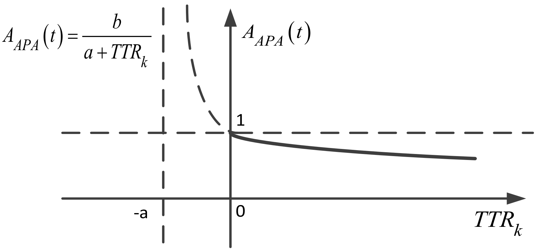
(2) When the kth $(k\ge 1)$ fault occurs, the items in Equation (4) are all constants except for $TT{R}_k$, so $A_{APA}(t)$ varies only with the change of $TT{R}_k$, expressed by Equation (6). a, b respectively, denote the cumulative availability time and the cumulative time when the kth fault occurs and both of them are constants in this phase.

$$A_{APA}\left(t\right)=\frac{{\displaystyle \sum _{i=0}^{k-1}TB{F}_i}}{{\displaystyle \sum _{i=0}^{k-1}\left(TB{F}_i+TT{R}_i\right)}+TT{R}_k}=\frac{b}{a+TT{R}_k}$$

(6)

The varying curve of $A_{APA}(t)$ in this phase is shown with the solid line in Figure 1.

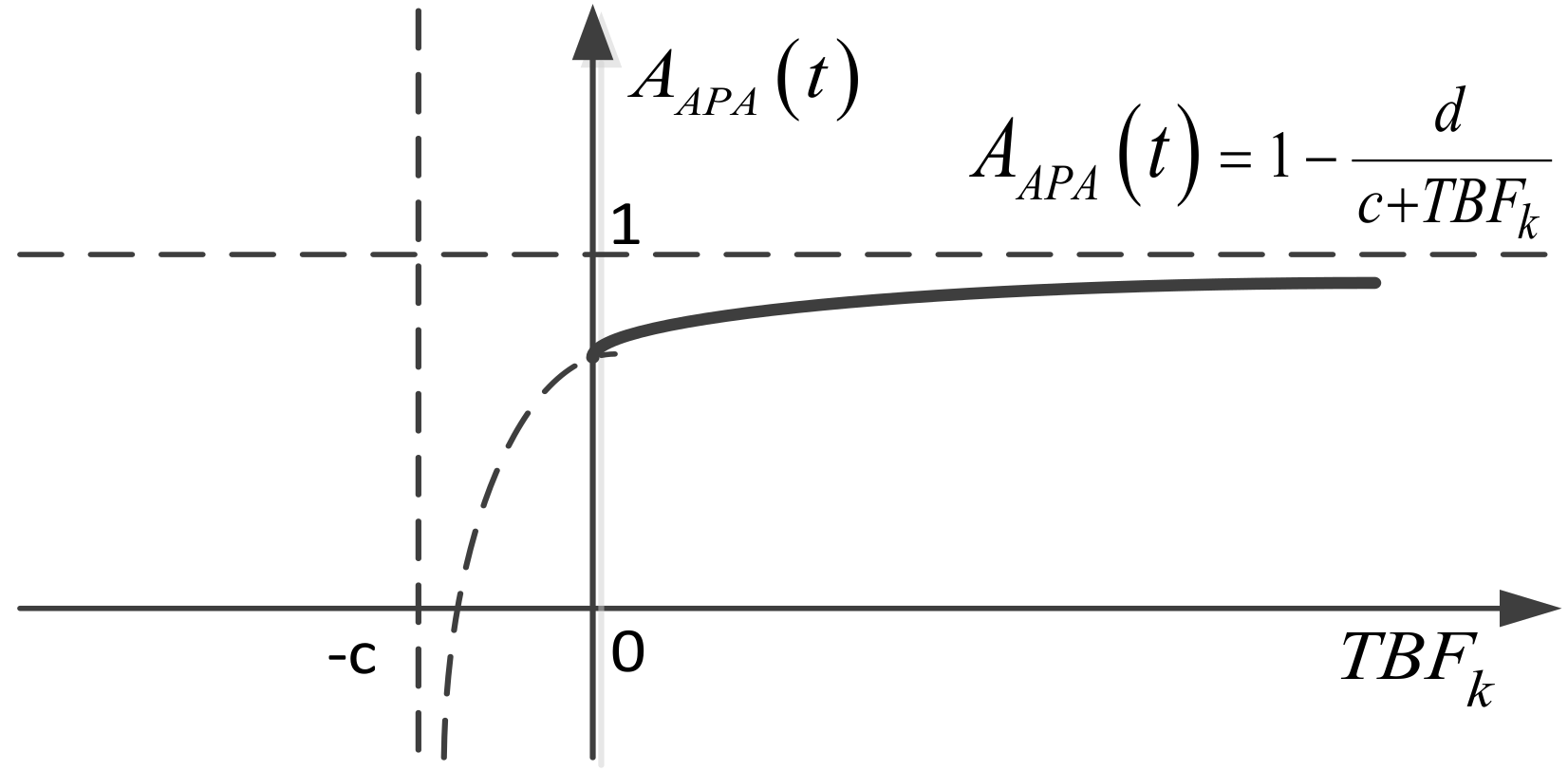
(3) When the channel returns to normal state from the kth failure, the items in Equation (4) are all constants except for $TB{F}_k$, so $A_{APA}(t)$ varies only with the change of $TB{F}_k$, expressed by Equation (7). c, d respectively denote the cumulative repair time and the cumulative time when the channel returns to normal state from the kth failure and both of them are constants in this phase.

$$A_{APA}\left(t\right)=1-\frac{{\displaystyle \sum _{i=0}^{k}TT{R}_i}}{{\displaystyle \sum _{i=0}^k\left(TB{F}_i+TT{R}_i\right)}}=1-\frac{d}{c+TB{F}_k}$$

(7)

The varying curve of $A_{APA}(t)$ in this phase is shown as the solid line in Figure 2.

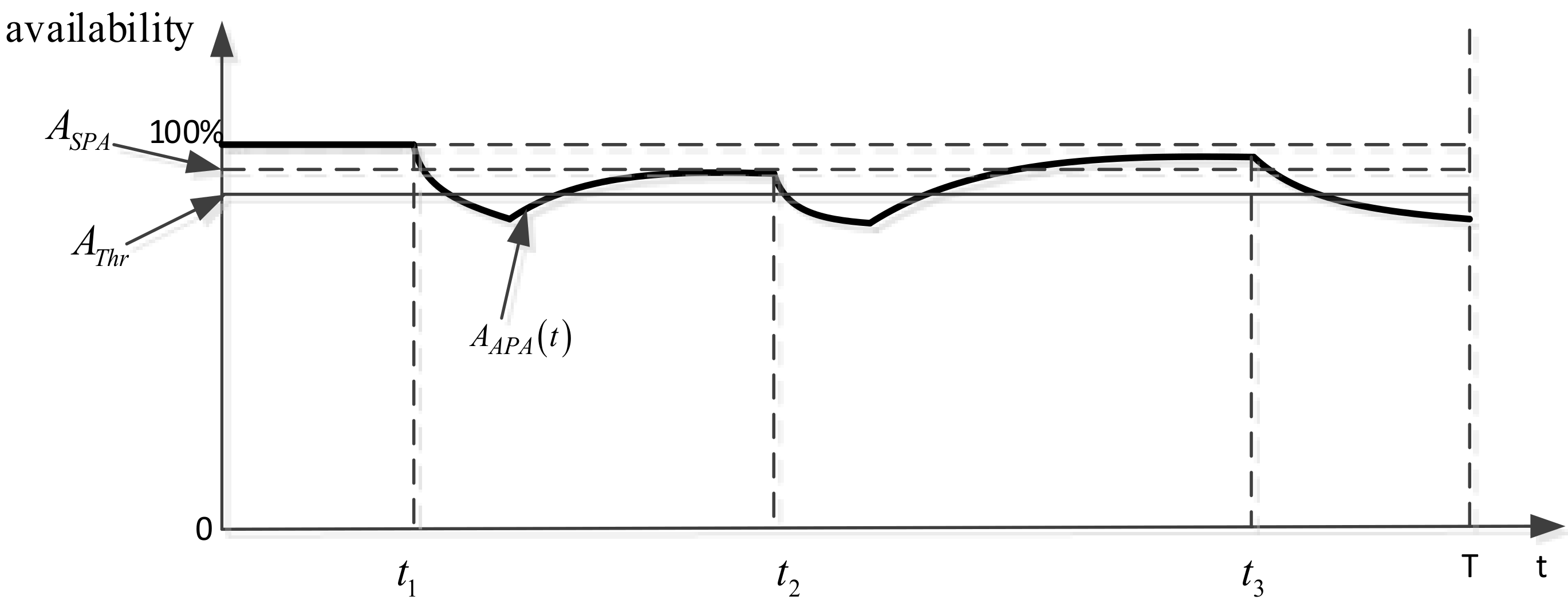
According to the analysis above, the varying curve of $A_{APA}(t)$ changes with the channel’s conversion process between normal states and failure states, as is shown in Figure 3. $A_{Thr}$ in Figure 3 denotes the availability threshold.

As shown in Figure 3, the differences between $A_{SPA}$, $A_{APA}(t)$ and $A_{Thr}$ are clearly illustrated. $A_{SPA}$ is the statistical mean value of $A_{APA}(t)$, which must be always greater than $A_{Thr}$ and is expressed as a horizontal dashed line in Figure 3. $A_{SPA}$ can be used to describe the overall availability of service channel from a global perspective but it cannot reflect the influence of each failure and repair time to the service.

$A_{APA}(t)$ is the actual availability of the service channel and its value can be calculated by (4) after each failure. However, since $TB{F}_i$, $TT{R}_i$, failure arrival rate and FN of each channel all have the nature of randomness, $A_{APA}(t)$ may be significantly higher than $A_{Thr}$ sometimes or may be lower than $A_{Thr}$ sometimes because of the sudden random failure. Therefore, the occurrence of SFE is inevitable.

If the degree of SCVR can be quantified, then the impact caused by SFE can be controlled, thereby the number and the duration of the impacted services can be reduced. To achieve the purpose, the SCVRD model is discussed and established in the following paragraphs.

3.2. SCVRD Model

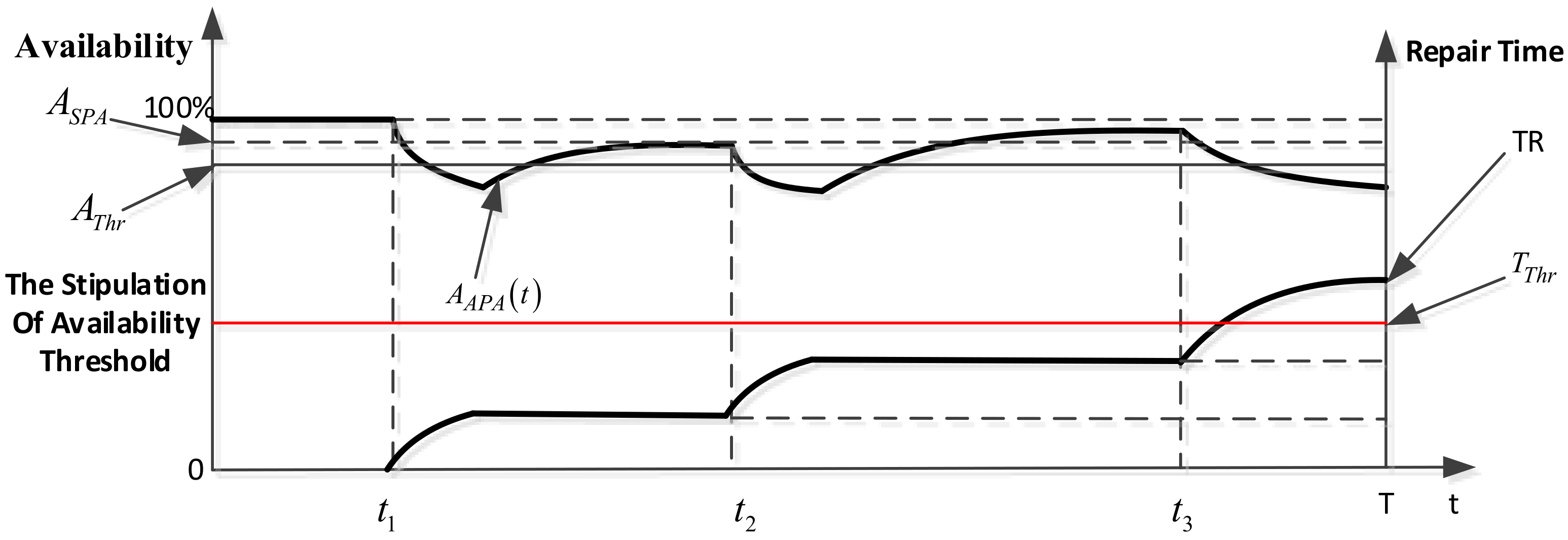
As shown in Figure 3, SCVRD which represents the probability of service channel violation risk $P_{SCVRD}$ can be expressed by Equation (8):

$$P_{SCVRD}=P\left(A_{APA}(t)<A_{Thr}\right)$$

(8)

However, SCVRD is hard to be accurately quantified and tracked due to the fluctuations of $A_{APA}(t)$. Thus, we introduce cumulative repair time TR and corresponding repair time threshold $T_{Thr}$ in the statistical period to describe the service channel violation risk.

$$TR={\displaystyle \sum _{i=0}^{+\infty }TT{R}_i}$$

(9)

$$T_{Thr}=\left(1-A_{Thr}\right)\times {\displaystyle \sum _{i=0}^{+\infty }(TB{F}_i+TT{R}_i)}$$

(10)

Then according to Equation (4), SCVRD can be quantified by Equation (11).

$$\begin{array}{l}{P}_{SCVRD}=P\left(A_{APA}\left(t\right)<A_{Thr}\right)\\ =P\left(\left(1-\frac{{\displaystyle \sum _{i=0}^{+\infty }TT{R}_i}}{{\displaystyle \sum _{i=0}^{+\infty }\left(TB{F}_i+TT{R}_i\right)}}\right)<A_{Thr}\right)=P\left(\frac{{\displaystyle \sum _{i=0}^{+\infty }TT{R}_i}}{{\displaystyle \sum _{i=0}^{+\infty }\left(TB{F}_i+TT{R}_i\right)}}>1-A_{Thr}\right)\\ =P\left({\displaystyle \sum _{i=0}^{+\infty }TT{R}_i}>\left(1-A_{Thr}\right)\times {\displaystyle \sum _{i=0}^{+\infty }\left(TB{F}_i+TT{R}_i\right)}\right)=P\left(TR>T_{Thr}\right)\end{array}$$

(11)

Thus, the probability of service channel violation risk based on availability is converted to the probability of cumulative repair time exceeding the corresponding repair time threshold in the statistical period. The equivalence relationship is shown in Figure 4.

Next, the characteristics of SCVRD will be further analyzed. By further analyzing Equation (4), we can find that $A_{APA}(t)$ is co-determined by FN of the service channel and each failure $TT{R}_i$. According to [23], TTR of $v_i$ and $e_{ij}$ is independent and they all obey the log-normal distribution as expressed by Equation (12). Therefore, TR subjects to the joint distribution of ${\displaystyle \sum {}_{i=1}^{\infty }}TT{R}_i$, which means that SFE is a random process and $P_{SCVRD}$ is a random probability model. Assume that FN of service channel obeys the Poisson distribution with average arrival rate λ, as expressed by Equation (13). Thus, the service channel violation risk caused by the kth failure $P_{SCVRD}(X=k,T{R}_k>T_{Thr})$ during the statistical period can be expressed by Equation (14):

$$f_i\left(t\right)=\frac{1}{\sqrt{2\pi }\cdot {\sigma }_i\cdot t}{e}^{-{\left(\ln \left(\mathrm{t}\right)-{\mathrm{\delta }}_i\right)}^2/2{\sigma }_i{}^2},$$

(12)

$$P_F\left(\mathrm{X}=k\right)=\frac{e^{-\lambda }{\lambda }^k}{k!},\lambda \in \left(0,1\right),k=1,2,\cdots$$

(13)

$${\mathrm{P}}_{SCVRD}\left(T{R}_X>T_{Thr},X=k\right)=P_F\left(X=k\right)\cdot P_R\left({\displaystyle \sum _{i=1}^{k}TT{R}_i}>T_{Thr}\right)$$

(14)

Because the failure occurrences of $v_i$ and $e_{ij}$ are independent, according to the conditional probability Equation and the n-fold convolution Equation, Equation (14) can be expanded to Equation (15):

$$\begin{array}{c}\begin{array}{l}{\mathrm{P}}_{SCVRD}\left(X=k,T{R}_X>T_{Thr}\right)\\ =P_F\left(X=k\right)\cdot P_T\left({\displaystyle \sum _{i=1}^{k}TT{R}_i}>T_{Thr}\right)\\ =P_F\left(X=k\right)\cdot \left(1-{\displaystyle {\int }_{T_{Thr}}^{+\infty }\cdots }{\displaystyle {\int }_{T_{Thr}}^{+\infty }\begin{array}{l}{f}_{T_k}\left(t_k\right)\cdots f_{T_2}\left(t_2\right)\cdot f_{T_1}\\ \left(D{T}_k-{\displaystyle \sum _{i=2}^k{t}_i}\right)d{t}_2\cdots d{t}_k\end{array}}\right)\end{array}\\ =\frac{e^{-\mathrm{\lambda }}{\mathrm{\lambda }}^k}{k!}\cdot \left(1-{\displaystyle {\int }_{T_{Thr}}^{+\infty }\cdots }{\displaystyle {\int }_{T_{Thr}}^{+\infty }\begin{array}{l}\frac{1}{\sqrt{2\pi }\cdot {\sigma }_k\cdot t_k}{e}^{-{\left(\ln \left({\mathrm{t}}_k\right)-{\mathrm{\delta }}_k\right)}^2/2{\sigma }_k{}^2}\cdots \frac{1}{\sqrt{2\pi }\cdot {\sigma }_k\cdot t_2}{e}^{-{\left(\ln \left({\mathrm{t}}_2\right)-{\mathrm{\delta }}_k\right)}^2/2{\sigma }_k{}^2}\cdot \\ \frac{1}{\sqrt{2\pi }\cdot {\sigma }_k\cdot \left(D{T}_k-{\displaystyle \sum _{i=2}^k{t}_i}\right)}{e}^{-{\left(\ln \left(D{T}_k-{\displaystyle \sum _{i=2}^k{t}_i}\right)-{\mathrm{\delta }}_k\right)}^2/2{\sigma }_k{}^2}\end{array}}d{t}_2\cdots d{t}_k\right)\end{array}$$

(15)

According to the total probability Equation, the Equation (15) can be expanded to (16).

$$\begin{array}{c}\begin{array}{l}{\mathrm{P}}_{SCVRD}\left(TR>T_{Thr}\right)\\ ={\displaystyle \sum _{k=1}^{+\infty }{P}_F\left(X=k\right)\cdot P_T\left({\displaystyle \sum _{i=1}^{k}TT{R}_i}>T_{Thr}\right)}\\ ={\displaystyle \sum _{k=1}^{+\infty }{P}_F\left(X=k\right)\cdot \left(1-{\displaystyle {\int }_{T_{Thr}}^{+\infty }\cdots }{\displaystyle {\int }_{T_{Thr}}^{+\infty }\begin{array}{l}{f}_{T_k}\left(t_k\right)\cdots f_{T_2}\left(t_2\right)\cdot f_{T_1}\\ \left(D{T}_k-{\displaystyle \sum _{i=2}^k{t}_i}\right){\mathrm{dt}}_2\cdots {\mathrm{dt}}_k\end{array}}\right)}\end{array}\\ ={\displaystyle \sum _{k=1}^{+\infty }\frac{e^{-\mathrm{\lambda }}{\mathrm{\lambda }}^k}{k!}\cdot \left(1-{\displaystyle {\int }_{T_{Thr}}^{+\infty }\cdots }{\displaystyle {\int }_{T_{Thr}}^{+\infty }\begin{array}{l}\frac{1}{\sqrt{2\pi }\cdot {\sigma }_k\cdot t_k}{e}^{-{\left(\ln \left({\mathrm{t}}_k\right)-{\mathrm{\delta }}_k\right)}^2/2{\sigma }_k{}^2}\cdots \frac{1}{\sqrt{2\pi }\cdot {\sigma }_k\cdot t_2}\\ e^{-{\left(\ln \left({\mathrm{t}}_2\right)-{\mathrm{\delta }}_k\right)}^2/2{\sigma }_k{}^2}\cdot \frac{1}{\sqrt{2\pi }\cdot {\sigma }_k\cdot \left(D{T}_k-{\displaystyle \sum _{i=2}^k{t}_i}\right)}\\ e^{-{\left(\ln \left(D{T}_k-{\displaystyle \sum _{i=2}^k{t}_i}\right)-{\mathrm{\delta }}_k\right)}^2/2{\sigma }_k{}^2}\end{array}}d{t}_2\cdots d{t}_k\right)}\end{array}$$

(16)

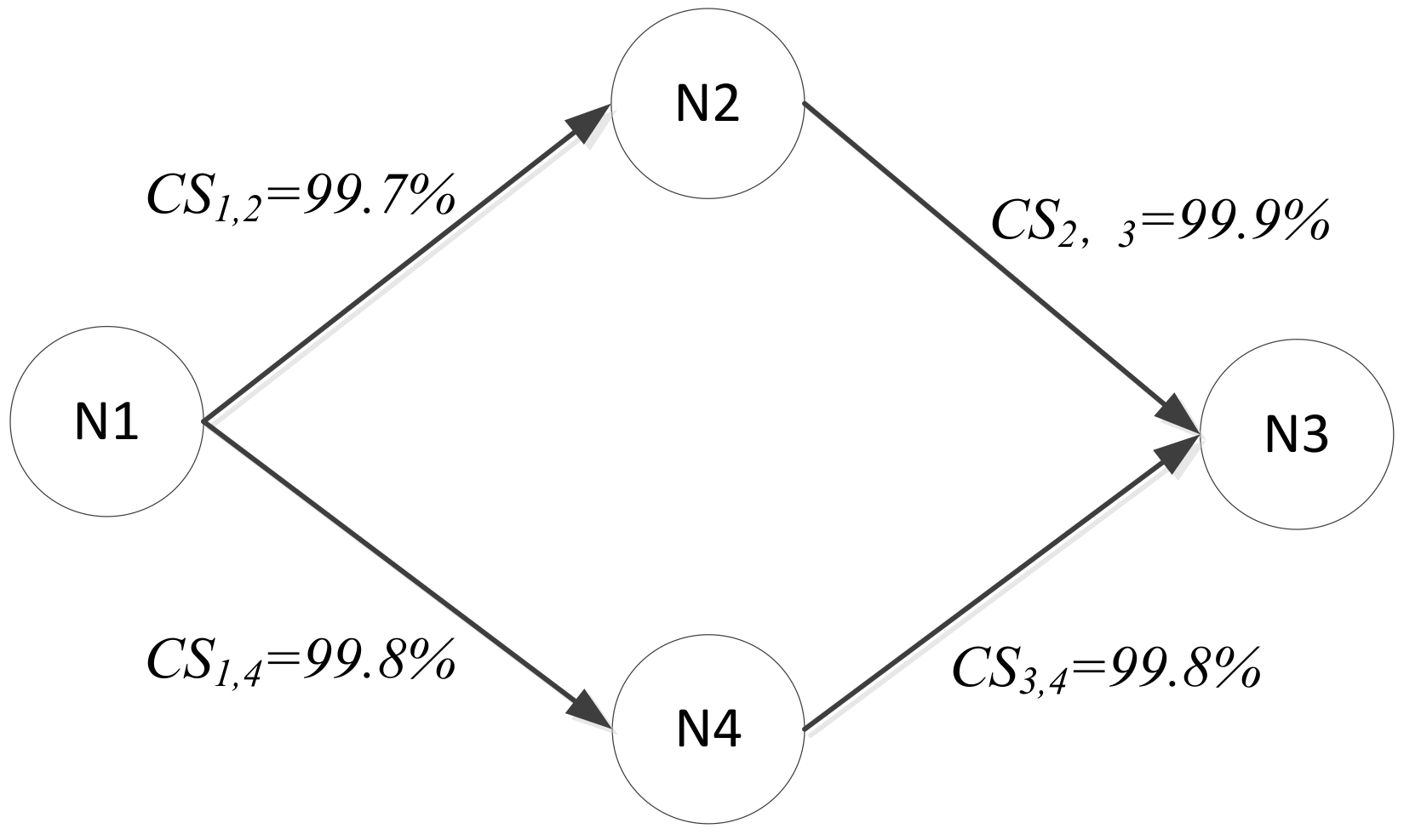
Figure 5 is an example to illustrate the difference between $P_{SCVRD}(TR>T_{Thr})$ and $A_{SPA}$ in the process of SCVRD quantization.

In Figure 5, an example for availability distribution diagram of the service channel violation risk is shown. There are two service channels named $S{C}_{N1-N2-N3}$ and $S{C}_{N1-N4-N3}$ with $A_{SPA}$ = 99.8%. Assume $T_{Thr}$ = 99.5%, the parameters of $S{C}_{N1-N2-N3}$ are $\left\{{\mathrm{\lambda }}_1=0.36,\left({\mathrm{\mu }}_1=1,{\mathrm{\delta }}_2=0.5\right)\right\}$ and the parameters of $S{C}_{N1-N4-N3}$ are $\left\{{\mathrm{\lambda }}_2=0.18,\left({\mathrm{\mu }}_2=2,{\mathrm{\delta }}_2=0.5\right)\right\}$. Then, according to (16), ${\mathrm{P}}_{SCVRD}\left(T{R}_{S{C}_{N1-N2-N3}}>0.72\right)=0.426$ and $P_{SCVRD}\left(T{R}_{S{C}_{N1-N4-N3}}>0.72\right)=0.389$ are found. During the calculation, we can find that $P_R\left(k\right)<{10}^{-6}$ when $k>10$. As a result, when $k\le 10$, the precision requirement can be satisfied and this result is consistent with the fact that the repair time cannot be infinitely small.

Through this example, it can be found that although the $A_{SPA}$ of both $S{C}_{N1-N2-N3}$ and $S{C}_{N1-N4-N3}$ are all higher than $A_{Thr}$, there is still a failure risk of about 0.389~0.426 for service channel. In addition, although the $A_{SPA}$ of $S{C}_{N1-N2-N3}$ and $S{C}_{N1-N4-N3}$ are the same, their failure risks are still different: ${\mathrm{P}}_{SCVRD}\left(T{R}_{Link1}>0.72\right)=0.426$ and ${\mathrm{P}}_{SCVRD}\left(T{R}_{Link2}>0.72\right)=0.389$. Compared to $A_{SPA}$, $P_{SCVRD}$ is more accurate to distinguish the differences of $A_{APA}(t)$ among the channels. Thus $P_{SCVRD}$ is more suitable in the quantization process of SFE.

4. Routing Mechanism Based on SCVRD

4.1. Approximate Transformation of Violation Risk Distribution

In the electric power communication network, $v_i$ and $e_{ij}$ have the relatively high $A_{SPA}$. It means that there are only several hours that the channel is in failure state during the thousands of hours’ execution. Then it can be assumed that TTR of $v_i$ and $e_{ij}$ will not overlapped. In addition, the failure of $v_i$ and $e_{ij}$ is independent. Here the node violation risk $P_{v_i}(TR>T_{Thr})$ is analyzed and the violation risk model of edge $P_{e_{ij}}(TR>T_{Thr})$ can be got this way. Here the node violation risk model is introduced. As to node $v_i$, the repair time $TT{R}_j,\begin{array}{c}\end{array}j=1,\mathrm{..}$ obey the log-normal distribution with parameters $\left({\mathrm{\mu }}_i,\begin{array}{c}\end{array}{\mathrm{\delta }}_i\right)$, because $TT{R}_j$ is a random variable, there is possibility that the $TT{R}_1$ of first failure may be bigger than $T_{Thr}$ and there also may be k failure occurs before ${\displaystyle \sum _{j=2}^k\left(TT{R}_j\right)}>T_{Thr}$. Therefore, from the total probability Equation we have:

$$\begin{array}{c}{\mathrm{P}}_{v_i}\left(TR>T_{Thr}\right)={\displaystyle \sum _{k=1}^{+\infty }{P}_F\left(X=k\right)\cdot P_T\left({\displaystyle \sum _{j=1}^{k}TT{R}_j}>T_{Thr}\right)}\\ ={\displaystyle \sum _{k=1}^{+\infty }\frac{e^{-\mathrm{\lambda }}{\mathrm{\lambda }}_i{}^k}{k!}\cdot \left(1-{\displaystyle {\int }_{T_{Thr}}^{+\infty }\cdots }{\displaystyle {\int }_{T_{Thr}}^{+\infty }\begin{array}{l}\frac{1}{\sqrt{2\pi }\cdot {\sigma }_i\cdot t_k}{e}^{-{\left(\ln \left({\mathrm{t}}_k\right)-{\mathrm{\mu }}_i\right)}^2/2{\sigma }_i{}^2}\cdots \\ \frac{1}{\sqrt{2\pi }\cdot {\sigma }_i\cdot t_2}{e}^{-{\left(\ln \left({\mathrm{t}}_2\right)-{\mathrm{\mu }}_i\right)}^2/2{\sigma }_i{}^2}\cdot \frac{1}{\sqrt{2\pi }\cdot {\sigma }_i\cdot \left(D{T}_k-{\displaystyle \sum _{i=2}^k{t}_j}\right)}\\ e^{-{\left(\ln \left(D{T}_k-{\displaystyle \sum _{i=2}^k{t}_j}\right)-{\mathrm{\mu }}_i\right)}^2/2{\sigma }_i{}^2}\end{array}}d{t}_2\cdots d{t}_k\right)}\end{array}$$

(17)

Equation (16) gives the probability distribution of violation risk $P_{SCVRD}$ but the distribution function is too complex to be a decision parameter. We will simplify the distribution function of ${\displaystyle \sum {}_{i=1}^k}TT{R}_i>T_{Thr}$ according to the FN probability generating function, $TT{R}_i$ moment generating function and their distribution functions. So that $P_{SCVRD}$ can be used as a decision parameter in the channel routing process. The detailed derivation process is described as follows. Assume that the probability generating function of FN is expressed by:

$$P_{FN}\left(z\right)=E\left(z^{FN}\right)={\displaystyle \sum _{k=0}^{+\infty }\left(z^k\cdot \frac{e^{-{\mathrm{\lambda }}_i}\cdot {\mathrm{\lambda }}_i{}^k}{k!}\right)},-1\le z\le 1$$

(18)

The moment generating function of TTR is expressed by:

$$M_{TTR}\left(t\right)=E\left(e^{t\cdot TTR}\right)={\displaystyle {\int }_{-\infty }^{+\infty }{e}^{{}^{t\cdot x}}\cdot f\left(x\right)\cdot dx}$$

(19)

$f\left(x\right)$ is the probability density function of TTR, then the moment generating function of down time (DT) is expressed by:

$$\begin{array}{l}{M}_{DT}\left(t\right)=E\left(e^{t\cdot S}\right)=E\left[e^{t\left(TT{R}_1+\cdots +TT{R}_k\right)}\right]\\ ={\displaystyle \sum _{k=1}^{+\infty }{P}_{FN}\left(N=k\right)\cdot E\left(e^{t\left(TT{R}_1+\cdots +TT{R}_k\right)}|N=k\right)}\\ ={\displaystyle \sum _{k=1}^{+\infty }{P}_{FN}\left(N=k\right)\cdot E\left({\displaystyle \prod _{i=1}^k{e}^{t\cdot TT{R}_i}}\right)}\end{array}$$

(20)

Since $TT{R}_i$ is independent and obeys the same log-normal distribution, making use of the nature that the mathematical expectation of the product of the independent random variables equals to the product of the mathematical expectation of each independent random variable, the Equation (20) can be converted into Equation (21):

$$\begin{array}{l}{M}_{DT}\left(t\right)={\displaystyle \sum _{k=1}^{+\infty }{P}_F\left(N=k\right)\cdot {\displaystyle \prod _{i=1}^{k}E\left(e^{t\cdot TT{R}_i}\right)}}\\ ={\displaystyle \sum _{k=1}^{+\infty }{P}_F\left(N=k\right)\cdot [M_{TTR}\left(t\right){]}^k}=E\left(M_{TTR}{\left(t\right)}^k\right)\end{array}$$

(21)

From Equations (18) and (21), we get:

$$M_{DT}\left(t\right)=E\left(M_{TTR}{\left(t\right)}^k\right)=P_{FN}\left(M_{TTR}\left(t\right)\right)$$

(22)

Equation (18) is simplified to:

$$P_{FN}\left(z\right)=e^{-{\mathrm{\lambda }}_i}\cdot {\displaystyle \sum _{k=0}^{+\infty }\left(\frac{{\left(z\cdot {\mathrm{\lambda }}_i\right)}^k}{k!}\right)}=e^{-{\mathrm{\lambda }}_i}\cdot e^{z\cdot {\mathrm{\lambda }}_i}=e^{{\mathrm{\lambda }}_i\cdot \left(z-1\right)}$$

(23)

From Equations (22) and (23), we get:

$$M_{DT}\left(t\right)=e^{{\mathrm{\lambda }}_i\cdot \left(M_{TTR}\left(t\right)-1\right)}$$

(24)

From (24), the relationship between the moment generating function of total channel violation time and the moment generating function $M_{TTR}\left(t\right)$ of single violation time is explicit. Then we use the k-order moments of TTR to expand the moment generating function $M_{DT}\left(t\right)$. The k-order origin moment of TTR is expressed as Equation (25) and $f\left(t\right)$ is probability distribution function of TTR.

$$E\left(TT{R}^k\right)={\displaystyle {\int }_{-\infty }^{+\infty }{t}^k\cdot }f\left(t\right)dt$$

(25)

From Equations (20) and (25), we get:

$$M_{TTR}\left(t\right)=1+\frac{m_1\cdot t}{1!}+\frac{m_2\cdot t^2}{2!}+\frac{m_3\cdot t^3}{3!}+\cdots$$

(26)

Then:

$$M_{DT}\left(t\right)=e^{{\mathrm{\lambda }}_i\cdot \left(M_{TTR}\left(t\right)-1\right)}=e^{{}^{{\mathrm{\lambda }}_i\cdot \left(\frac{m_1\cdot t}{1!}+\frac{m_2\cdot t^2}{2!}+\frac{m_3\cdot t^3}{3!}+\cdots \right)}}$$

(27)

Let $Y=\frac{DT-{\mathrm{\lambda }}_i\cdot m_1}{\sqrt{{\mathrm{\lambda }}_i\cdot m_2}}$, $m_k$ represents the k-order origin moment of TTR and substituting Y into $M_Y\left(t\right)={\rm E}\left(e^{t\cdot Y}\right)$, then the moment generating function of Y is expressed as Equation (28):

$$M_Y\left(t\right)=e^{{\mathrm{\lambda }}_i\cdot \left[M_{TTR}\left(\frac{t}{\sqrt{{\mathrm{\lambda }}_i\cdot m_2}}\right)-1\right]-\frac{{\mathrm{\lambda }}_i\cdot m_1\cdot t}{\sqrt{{\mathrm{\lambda }}_i\cdot m_2}}}$$

(28)

From Equation (26), we get:

$$M_{TTR}\left(\frac{t}{\sqrt{{\mathrm{\lambda }}_i\cdot m_2}}\right)-1=\frac{m_1\cdot t}{\sqrt{{\mathrm{\lambda }}_i\cdot m_2}}+\frac{m_2\cdot t^2}{2{\mathrm{\lambda }}_i\cdot m_2}+\frac{m_3\cdot t^3}{6{\left({\mathrm{\lambda }}_i\cdot m_2\right)}^{3/2}}+\frac{m_4\cdot t^4}{24{\left({\mathrm{\lambda }}_i\cdot m_2\right)}^2}+\cdots$$

(29)

Put Equation (29) into Equation (28), we get:

$$M_Y\left(t\right)=e^{\frac{1}{2}\cdot t^2+\frac{m_3}{6\sqrt{{\mathrm{\lambda }}_i}\cdot {\left(m_2\right)}^{3/2}}\cdot t^3+\frac{m_4}{24{\mathrm{\lambda }}_i\cdot {\left(m_2\right)}^2}\cdot t^4+\cdots }$$

(30)

When ${\mathrm{\lambda }}_i\to \infty$,

$$\underset{{\mathrm{\lambda }}_i\to \infty }{\lim }{M}_Y\left(t\right)=e^{t^2/2}$$

(31)

Since the moment generating function of the standard normal distribution is $M_{N\left(0,1\right)}\left(t\right)=e^{t^2/2}$, Equation (31) means that the moment generating function of Y converges to the moment generating function of standard normal distribution. Because the probability generating function or moment generating function of random variable is corresponding to its distribution function, the distribution function of Y converges to the standard normal distribution $N(0,1)$. Thus, the service channel violation risk $P_R$ is approximately calculated by converting $Y=\frac{DT-{\mathrm{\lambda }}_i\cdot m_1}{{\mathrm{\lambda }}_i\cdot m_2}$ and standard normal distribution function $\mathsf{\Phi }\left(Y\right)$, which is expressed by Equation (32)

$$P_R\left(DT>T_{Thr}\right)\approx \mathsf{\Phi }\left(\frac{T_{Thr}-{\mathrm{\lambda }}_i\cdot m_1}{{\mathrm{\lambda }}_i\cdot m_2}\right)$$

(32)

By Equation (32), the expected value and variance of log-normal distribution can be respectively calculated as:

$$E\left(X\right)=e^{{\mathrm{\mu }}_i+\frac{{\sigma }_i{}^2}{2}}$$

(33)

$$Var\left(X\right)=e^{2{\mathrm{\mu }}_i+{\sigma }_i{}^2}\left[e^{{\sigma }_i{}^2}-1\right]$$

(34)

${\mathrm{\mu }}_i$ and ${\sigma }_i$ are the expected value and variance of normal distribution. According to $Var(X)=E(X^2)-{[E(X)]}^2$, we get:

$$m_1=E\left(X\right)=e^{{\mathrm{\mu }}_i+\frac{{\sigma }_i{}^2}{2}}$$

(35)

$$m_2=E\left(X^2\right)=Var\left(X\right)+{\left(E\left(X\right)\right)}^2=e^{{\mathrm{\mu }}_i+\frac{{\sigma }_i{}^2}{2}}+e^{2{\mathrm{\mu }}_i+{\sigma }_i{}^2}\left[e^{{\sigma }_i{}^2}-1\right]$$

(36)

Substituting Equations (35) and (36) into Equation (32), we get:

$$P_R\left(DT>T_{Thr}\right)\approx \mathsf{\Phi }\left(\frac{T_{Thr}-{\mathrm{\lambda }}_i\cdot e^{{\mathrm{\mu }}_i+\frac{{\sigma }_i{}^2}{2}}}{{\mathrm{\lambda }}_i\cdot \left(e^{{\mathrm{\mu }}_i+\frac{{\sigma }_i{}^2}{2}}+e^{2{\mathrm{\mu }}_i+{\sigma }_i{}^2}\left[e^{{\sigma }_i{}^2}-1\right]\right)}\right)$$

(37)

Equation (37) gives the approximate method to calculate the violation risk of $v_i$, which can be used as the decision-making parameter to select the route with minimum violation risk for service channel.

4.2. SCVRD Based Routing (SCVRD-R) Algorithm

Since the service channel is composed of $v_i$ and $e_{ij}$, $v_i$ and $e_{ij}$ is independent of each other, the service channel violation risk minimization problem $Min\left(P_R\left(DT>T_{Thr}\right)\right)$ can be converted into the shortest path problem with $SCVRD(v_i)$ and $SCVRD(e_{ij})$ as the weight. To solve this problem, SCVRD-R algorithm based on Dijkstra is proposed in this paper. Here the nodes and edges that service channel passes are all called as channel section (CS), then in order to simplify the description of the algorithm, $SCVRD(v_i)$ and $SCVRD(e_{ij})$ will be denoted as $SCVRD(C{S}_i)$. The steps of SCVRD-R algorithm are described as follows. Figure 6 is the flowchart of SCVRD-R Algorithm 1.

Algorithm 1.SCVRD-R Algorithm.

(1) Initialize the graph G(N,E) and the aTTRibute vector of service (s, d, B, A, r).     s, d, B, A and r(s,d) denote the source node, destination node, bandwidth requirements, availability threshold and the violation risk degree between s and d respectively. $r_0(s,d)=0$. When there is no channel between s and d, r(s,d) $+\infty$. Set S = {s}, D = G-s.   (2) If the bandwidth of any path in the graph G(N,E) does not meet the bandwidth requirements B, then the path is deleted from G(N,E). Thus, a new sub-graph G’(N,E) is generated.   (3) For each $C{S}_i\in G(N,E),$     Calculate the probability of violation risk $P_{C{S}_i}(TR>T_{Thr})$ according to Equation (37).   End for each.   (4) Choose the $C{S}_i$ with minimum violation risk probability $P_{C{S}_i}$ from D, then $D=D-C{S}_i$, $S=S+C{S}_i$.   (5) Take $C{S}_i$ as the middle path, if the violation risk from s to $C{S}_k$ shrinks, then modify $r(s,C{S}_k)$.   (6) Repeat step 4 and step 5 until $C{S}_i=d$.   (7) If the new route is different from the original one, then a new service channel is created.   Repeat Step 2 to Step 7.

5. Simulation and Results

In this paper, two ways have been used to analyze the performance of the algorithm. Firstly, the Monte Carlo analysis method is adopted to simulate the random failures of service channel. The result of this method is compared to AAR-OS algorithm. Secondly, based on the backbone topology of one provincial electric power company, we randomly generate the distribution parameters of failure arrival rate and repair time for $v_i$ and $e_{ij}$. Then the performance of SCVRD-R algorithm, AAR-OS algorithm and risk-aware provisioning (RAP) algorithm [23] is compared under the intensity of 10 kinds of services.

5.1. Monte Carlo Experiment Based on Four Nodes

As shown in Figure 5, there exist two service channels from node N1 to node N3 named $S{C}_{N1-N2-N3}$ and $S{C}_{N1-N4-N3}$, whose availability are both 99.7%. Now from N1 to N3, there is a kind of power communication service $S_i$ with availability requirement of 99.5%. The monthly failure number and the repair time of $S{C}_{N1-N2-N3}$ and $S{C}_{N1-N4-N3}$ are respectively generated according to the parameters $\left\{{\mathrm{\lambda }}_1=0.36,\left({\mathrm{\mu }}_1=1,{\mathrm{\delta }}_2=0.5\right)\right\}$ and $\left\{{\mathrm{\lambda }}_2=0.18,\left({\mathrm{\mu }}_2=2,{\mathrm{\delta }}_2=0.5\right)\right\}$.

To reduce the impact on experiment results which is brought by our algorithm’s random nature, we get the probability of service channel violation risk through repeating experiment 10,000 times and the method that the channel monthly statistical average failure times are divided by the experiment times. The statistical average data and the routing results of two algorithms are shown in

Table 1. Comparison Table of Violation Risk and Routing Result.

. In the Table 1, the thick arrows denote the route selected by SCVRD-R algorithm, while the thin arrows denote the route selected by AAR-OS algorithm.

From Table 1, it can be seen that the violation risk of the two channels are fluctuating. If AAR-OS algorithm is adopted, even when the violation risk of $S{C}_{N1-N2-N3}$ is lower than $S{C}_{N1-N4-N3}$ (for example on month 6 and 7), AAR-OS will always choose the channel $S{C}_{N1-N4-N3}$ for the service $S_i$ because the channel $S{C}_{N1-N4-N3}$ has slightly higher statistical availability than $S{C}_{N1-N2-N3}$. If SCVRD-R algorithm proposed in this paper is adopted, then the lower risk route will be selected for $S_i$ according to the change of the violation risk value. Thus, the number of the service violation will be reduced and its $A_{APA}(t)$ will be enhanced.

5.2. Network Simulation

The network simulation scenario is set up based on the backbone network topology of one provincial electric power company, as shown in Figure 7. The raw data about topology, business and actual routing are all provided by this electric power company because of the research cooperation between this company and our research team.

The network simulation topology contains 74 nodes and 104 edges. The purpose of the simulation experiment is to compare the failure rate of the service channel routed by SCVRD-R algorithm, AAR-OS algorithm and RAP algorithm in 12 months in

Table 2. Service Intensity Distribution Table.

Intensity	1	2	3	4	5	6	7	8	9	10
Number of Service	[1,3]	[3,5]	[5,8]	[8,10]	[10,13]	[13,15]	[15,18]	[18,20]	[20,25]	[25,30]

.

Here, we divide 30 services into ten kinds of service intensities as an instance to evaluate the algorithm performance in the different ten service intensities. However, the partition of service intensities is not only this one way. Assume that the service is generated between nodes in 2 hops of 14 aggregation nodes (marked with circle in Figure 7) and the services have the same availability threshold of 99.5%. The failure arrival rates of nodes and edges are randomly generated in the interval of [0.006, 1.5] and their repair time are randomly generated in the interval of [0.4, 0.003]. The service channel failure rate is calculated using the ratio between the number of failure service channels and the number of total service channels. The bandwidth of each optical cable is 5GB. At present the bandwidth in the electric power communication transmission network is redundant. Besides, the SDH electric power communication service channel uses fixed bandwidth. So, we temporarily do not consider the variable bandwidth of cable.

The simulation results are shown in Figure 8, which shows that the average service channel failure rate of SCVRD-R algorithm is respectively about 15% and 6% lower than that of AAR-OS algorithm and RAP algorithm under the different service intensities. Other service intensities are similar. The failure rate in the various service intensities has nothing to do with the change of month, just randomly changes within months. The temporal resolution of data is not necessarily fixed for month, which means that week or other durations can also be set as the temporal resolution of data.

5.2.1. Service Channel Failure Rate Comparison

Figure 8a shows the service channel failure rates of SCVRD-R algorithm, AAR-OS algorithm and RAP algorithm in 12 months under service intensity 1. Because SCVRD-R algorithm finds route according to SCVRD, the service channel can adjust the route based on the distribution of failure arrival rate and TTR to avoid the fault paths, which can reduce the service channel failure rate. The results in Figure 8b,c are similar to the results in Figure 8a.

5.2.2. Failure Rate Comparison Under the Saturation Status

Figure 8d shows the service-channel failure rate of SCVRD-R algorithm, AAR-OS algorithm and RAP algorithm in 12 months under service intensity 4. Under this service strength, the traffic carried by parts of the optic cables may reach the bandwidth limit and the network will begin to be the saturation status. In this case, the service channel with low SCVR cannot carry the service which is transferred from the service channel with relatively high SCVR. Then, parts of the services cannot select the route according to the lowest violation risk, resulting in the ascending service channel failure rate. In addition, with the growing of number of services, the ability of these three algorithms to control $A_{APA}(t)$ and SCVRD of channels is gradually weakened. So, the results of the failure rate turn to convergence and will finally converge to the failure rate without routing risk control as the number of services grows.

6. Conclusions

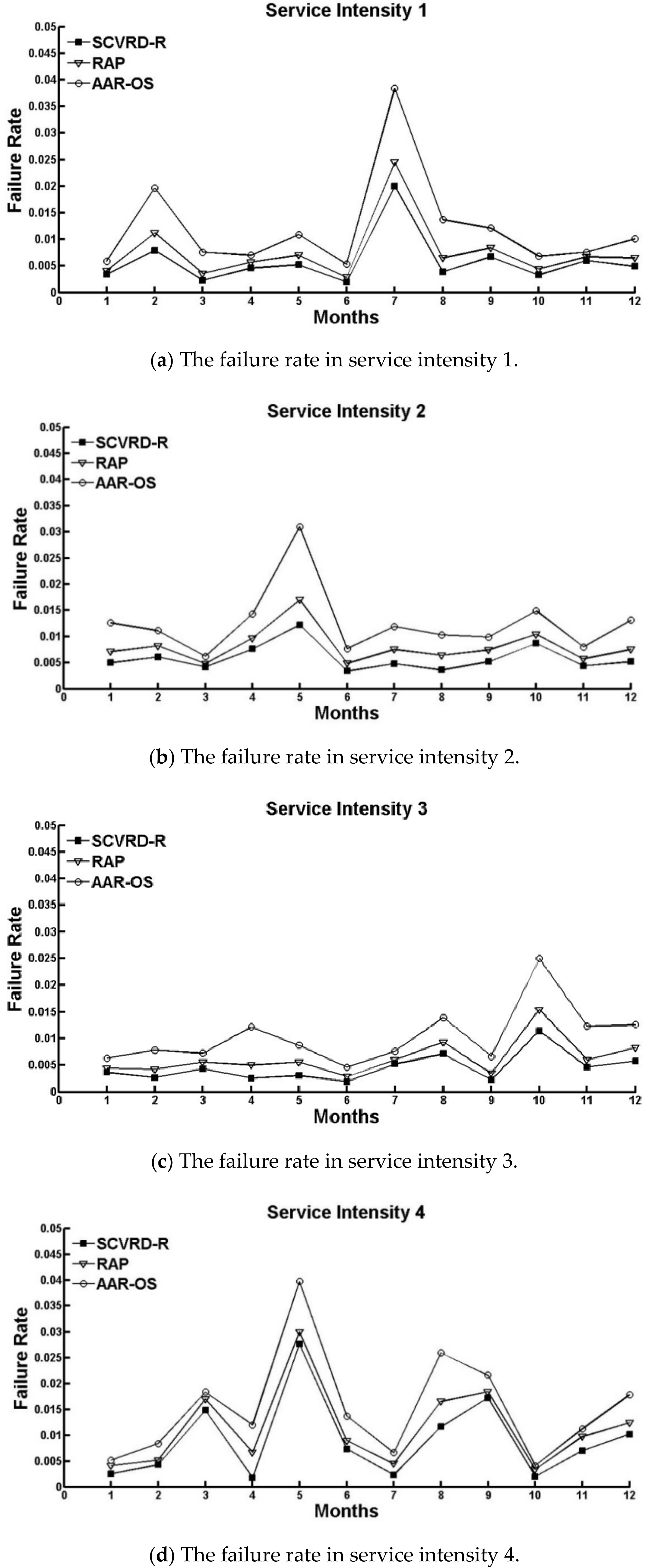
On account of the problems in electric power communication service route planning, a probability model of service channel violation risk, named SCVRD model, is proposed in this paper. Generally, the $A_{SPA}$ is calculated by mean value and $A_{APA}(t)$ is calculated based on some assumption, both of them cannot precisely track the violation risk change of service channel which is caused by the random failure under random TTR condition. To solve this problem, we deduce SCVRD model from the service channel violation risk model which is usually denoted by $A_{APA}(t)$ and denote SCVRD model by the probability of service channel cumulative failure duration exceeding the prescribed duration. The deduction is proved and then SCVRD model is simplified using mathematical method. Based on SCVRD, a service channel violation risk degree routing algorithm, named SCVRD-R algorithm, is proposed to reduce the risk caused by random failure of transmission equipment and optical cable and improve the availability of electric power communication service. Finally, the simulation results show that the average service channel failure rate of AAR-OS algorithm and RAP algorithm are respectively reduced by 15% and 6%.

In future work, we plan to further investigate how the failure rate convergence changes when optic cables reach the bandwidth limit. Furthermore, we intend to figure out the accurate numerical relationship among service intensity, service channel bandwidth and failure rate convergence to actually guide the service routing planning and optimization in electric power communication network. In many cases, the success of smart grid depends on their ability to support real-time decision-making. Therefore, we would make further efforts on the exploration of our proposed methodology in medium and short-term planning scenarios.