Performance Analysis of Hybridization of Heuristic Techniques for Residential Load Scheduling

Abstract

With the emergence of the smart grid, both consumers and electricity providing companies can benefit from real-time interaction and pricing methods. In this work, a smart power system is considered, where consumers share a common energy source. Each consumer is equipped with a home energy management controller (HEMC) as scheduler and a smart meter. The HEMC keeps updating the utility with the load profile of the home. The smart meter is connected to a power grid having an advanced metering infrastructure which is responsible for two-way communication. Genetic teaching-learning based optimization, flower pollination teaching learning based optimization, flower pollination BAT and flower pollination genetic algorithm based energy consumption scheduling algorithms are proposed. These algorithms schedule the loads in order to shave the peak formation without compromising user comfort. The proposed algorithms achieve optimal energy consumption profile for the home appliances equipped with sensors to maximize the consumer benefits in a fair and efficient manner by exchanging control messages. Control messages contain energy consumption of consumer and real-time pricing information. Simulation results show that proposed algorithms reduce the peak-to-average ratio by 34.56% and help the users to reduce their energy expenses by 42.41% without compromising the comfort. The daily discomfort is reduced by 28.18%.

1. Introduction

To make an advanced and automated energy management and distribution system, the smart grid incorporates new, smart and intelligent technologies. Smart controllers and relays along with intelligent software tools are used for data management. The best feature of the smart grid is the two-way communication between power companies and consumers. This two-way communication of information enables the utility companies and consumers to control their load, reduce bill and peak-to-average ratio (PAR). The gain of user comfort (UC), implementation of user preferences and integration of renewable energy (RE) is another advantage. The addition of these new and intelligent technologies in the next generation power grid is going to be incorporated across the entire power system. The smart grid incorporates new technologies from generation, transmission and distribution of power consumption at the consumer’s side. These technologies are used for the purpose of enhancing the safety, reliability and efficiency of the power system.

Residential and commercial buildings consume 50% of the global power [1]. The active collaboration and energy sharing by buildings and homes are not included in the present electricity system. All the energy management efforts carried out are less effective and their efficiency is affected by this. The smart grid enables the next generation energy efficiency and sustainability. In this kind of architecture as discussed above, the aggregation of houses acts as an intelligent collaboration of networked system, whereas, in the conventional system, they act as passive and isolated units [2].

With the help and cooperation of smart grid technologies, investment in a traditional grid can be changed or reduced by implementing demand side management (DSM) rules. The participants of the DSM or demand response (DR) programs try to reduce their energy utilization at certain instances showing a little flexibility. By offering flexibility, consumers achieve benefits [3].

Since 1982, the increase in peak electricity demand and electricity usage has increased from the growth in electric appliances and increasing demand of power by industry. The increase is almost 25% by each year according to the USA department of energy [4]. Moreover, considering the residential sector in the USA, the electricity sales are expected to increase 24% from 2011 to 2040 [5]. Peak energy demand is expected to be far more than the available transmission, generation and distribution capability of the existing grid. This dilemma can be solved by enhancing the existing transmission capability, decreasing peak load, increasing distributed generation and exploring new methods of energy generation such as renewable energy sources (RESs). Researchers are trying to expand traditional grid infrastructure to meet new challenges; however, it is a very expensive job [4].

There are also monitory benefits added to the physical system consideration. The peak power stations can be eliminated by reducing the load during peak hours. This ensures decrease in cost of electricity for consumers. As an example, during the California energy crisis of 2000–2001, a 5% peak demand reduction decreased the highest wholesale prices by 50% as stated in [6]. The authors attempt to decrease peak load demand by intelligent and smart coordination amongst customer’s appliances scheduling. The peak demand is avoided by scheduling the appliances in low peak hours and thus benefiting both the consumers and utility companies [7].

There is an emerging trend toward scheduling the load of residential homes, reducing electricity cost and balancing the energy consumption across 24 h of a day. The use of microgrid (MG) comprising of RESs are in spotlight. Normally, photovoltaic (PV) source, wind turbines and micro combined heat and power generators are used. The current power generation system is in a transition state to become a large scale distributed power generation system. This transition state to smart grid will be completed with the addition of distributed RESs [8,9].

A smart grid also supports changing electricity prices and this change is according to the dynamic status of electric power demand and generation system. The smart grid is now a promising method for the RE generation, resources management, use in the context of increasing energy demand and increasing prices [10].

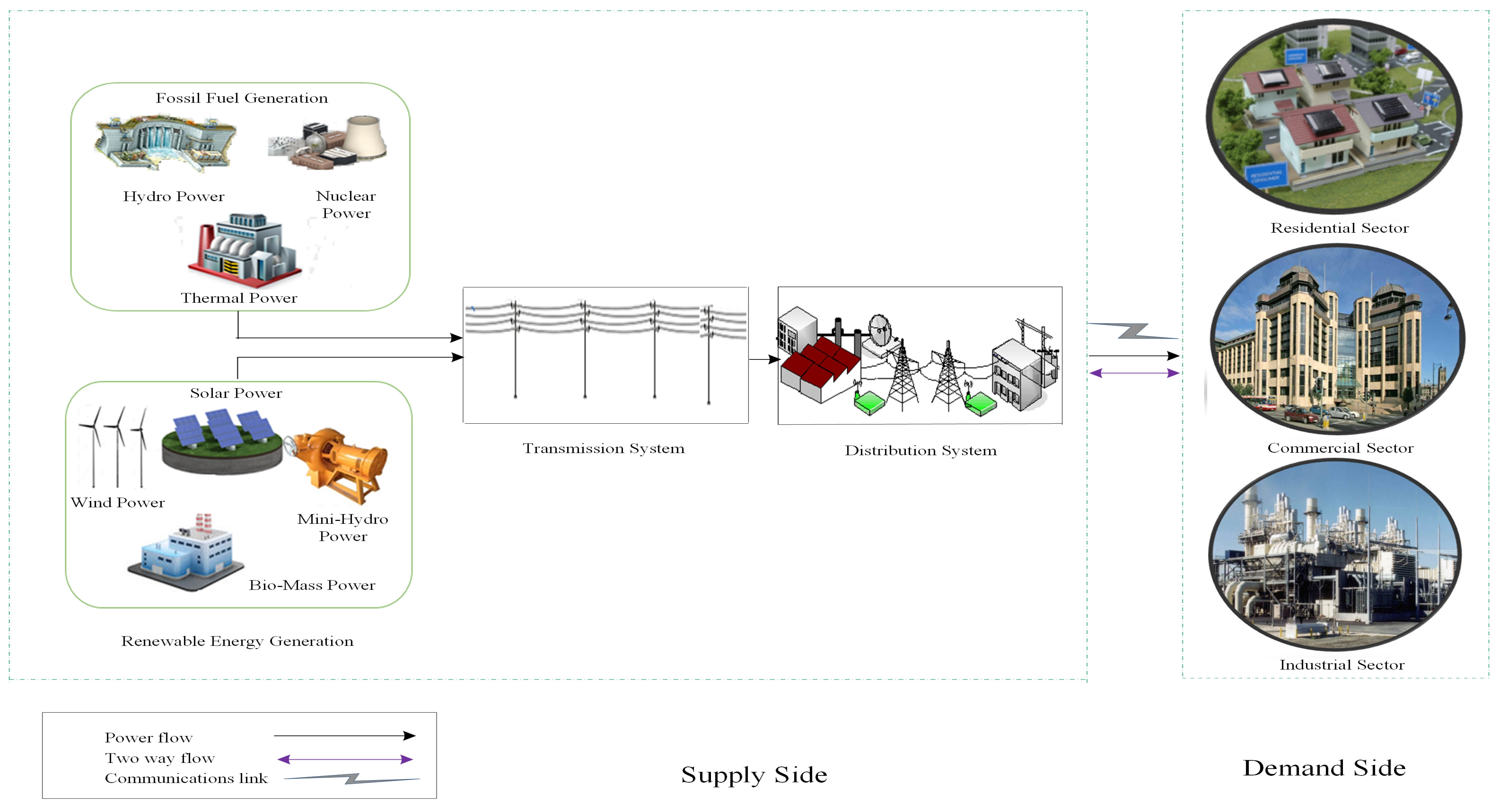
The recent smart appliances and smart grid technologies enable residential and commercial sector to use power efficiently using smart grid features. Such electrical appliances have the capability to make their operation according to the changing electricity prices. Peak load management can reduce the cost of electricity consumption. 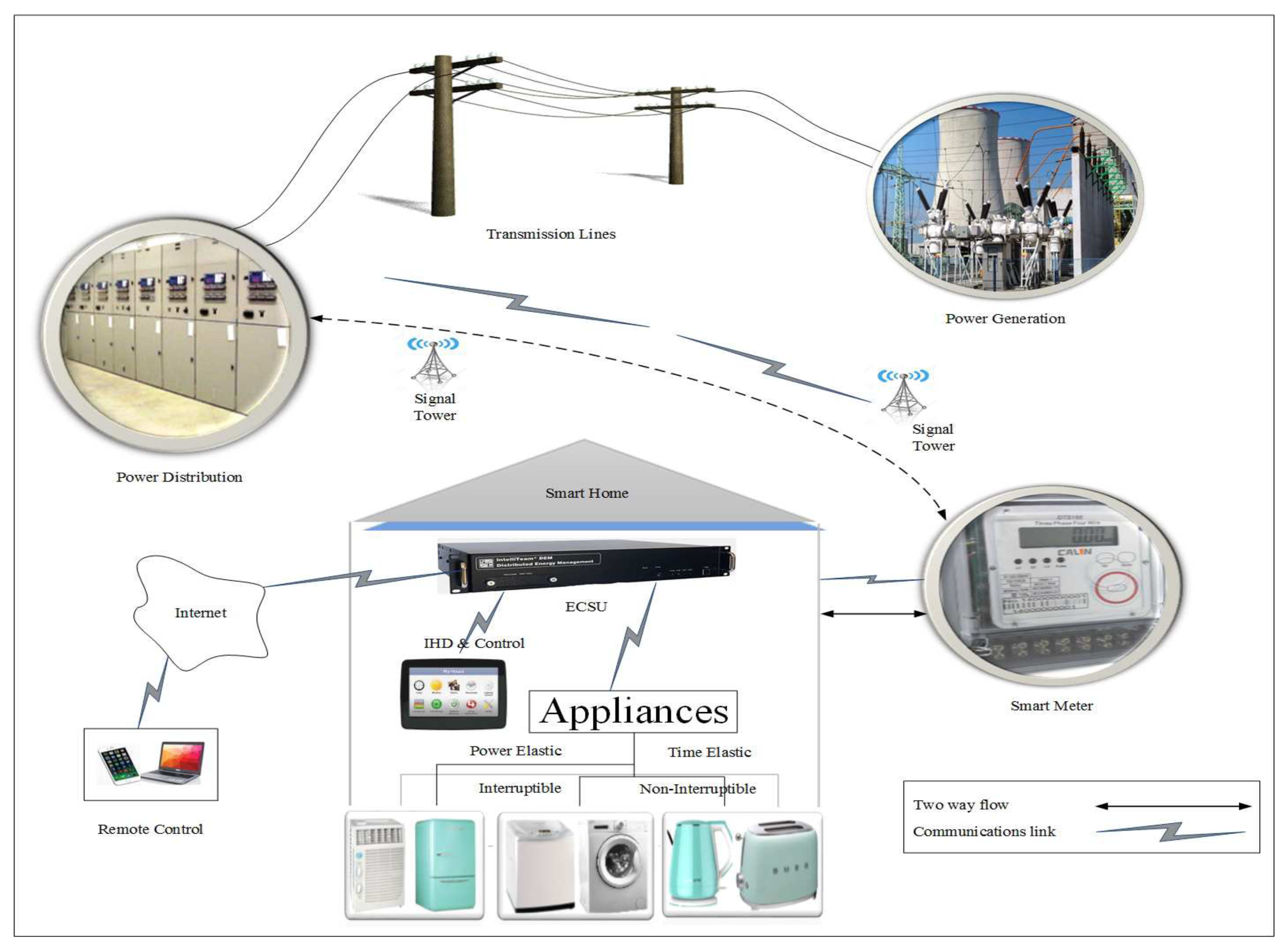The reliability of electric grid can be improved by using smart appliances and their load management characteristics knowing every minute details of each appliance [11]. An abstract view of power flow for supply and demand side is presented in Figure 1.

The researchers are trying to add intelligence for energy management in order to improve the efficiency, comfort, convenience in services and home-based health-care support [12,13]. There are many articles, in which especially smart homes energy management systems considering energy efficiency and load management are discussed [14,15,16,17]. Most of the literature considers reduction of cost via load management by following variations in electricity prices. This paper proposes a novel approach for appliances scheduling in residential buildings which gives a detailed smart home energy management system solution. This approach minimizes the overall daily electricity cost of home appliances.

In this work, residential load is scheduled using DSM for smart homes. Considering smart power system for consumers, where a common energy source is used, each consumer uses smart meter and energy consumption scheduling unit (ECSU). The electric grid and smart meter is connected via advanced metering infrastructure (AMI). The AMI communicates between the electric grid and smart meter. Four algorithms are proposed, i.e., genetic teaching learning based optimization (GTLBO), flower pollination teaching learning based optimization (FTLBO), flower pollination BAT (FBAT) and flower pollination genetic algorithm (FGA). These proposed algorithms are used to schedule the load for reducing electricity cost, user discomfort and PAR. Simulation results show that proposed techniques perform better as compared to the existing techniques. However, there is trade-off between cost and user discomfort. The discomfort decreases with the increasing cost and increases with decreasing cost. The list of the acronyms are listed in

Table 1. Acronyms.

Symbol	Description	Symbol	Description
A	Set of appliances	$E_T^{pe}$	Total energy consumption of power elastic appliances
$A_e^t$	Set of time elastic appliances	$E_c^a\left(t\right)$	Energy consumption of interruptible appliances
$A_e^p$	Set of power elastic appliances	$P_r^a$	Power rating of interruptible appliances
$S_t^i$	Current position of an appliance i	$E_T^a$	Total energy consumption of interruptible appliances
$S_{t+1}^i$	Position of appliance at the next time slot	$E_c^b\left(t\right)$	Energy consumption of non-interruptible appliances per time slot
$T_s^o$	ON time	$P_r^b$	Power rating of non-interruptible appliances
$\beta$	Operation end time	$E_T^b$	Total energy consumption by $\beta$ appliances
$\alpha$	Operation start time	$C_T^{pe}$	Total cost of power elastic appliances
$r_t^n$	Number of remaining time slots	$\rho$	Power rating
$w_t^n$	Number of waiting time slots	$C_T^{te}$	Total cost of time elastic appliances
$X_t$	ON/OFF status	$w_i$	Waiting time of appliance i
$p_{max}^i$	Maximum power of appliance i	$t_i$	Time of appliance i
$p_{min}^i$	Minimum power of appliance i	${\alpha }_i$	Start appliance i of set $\alpha$
$\rho \left(L^t\right)$	Combined electricity price at time slot t	${\beta }_i$	End time slot of Appliance i
$R_t$	Real-time price	$C_T$	Total cost of all appliances
$b_t$	Electricity price when IBR threshold exceeded	$E_T$	Total energy consumption of all appliances
$L^t$	Total load	$M{D}_i$	Mean difference
$L_{th}$	Threshold of load	$Mea{n}_{new}$	Outcome of the best learner
$E_c^j\left(t\right)$	Energy consumption of power elastic appliances per time slot	$r_i$	Random number between 0 and 1
$P_r^j$	Power rating of power elastic appliances	$T_{factor}$	Teaching factor
$E_T^{te}$	Total energy consumption of time elastic appliances

.

The rest of the paper is organized as follows: related work is discussed in Section 2. Discussion about the proposed system model is provided in Section 3. Section 4 explains the problem formulation using a mathematical technique called knapsack. In Section 5, optimization techniques are explained, In Section 6, simulation results and discussion have been provided. In Section 7, conclusions, future work and references are presented.

2. Related Work

A lot of research has been done on residential load scheduling, DSM for smart homes and home energy management (HEM). These are major trends in smart grid research domains.

In [18], authors discussed HEM controller for the residential load. Moreover, they used four algorithms for the bill and PAR reduction, i.e., the genetic algorithm (GA), binary particle swarm optimization (BPSO), wind driven optimization (WDO), bacterial foraging optimization algorithm (BFOA) and genetic BPSO (GBPSO). The authors achieved 34% PAR and 36% cost reduction. The cost for single, ten and fifty homes are calculated using the above techniques. However, the authors did not consider the UC and user preferences.

  A mixed integer programming optimization (MIPO) algorithm is proposed in [19] for scheduling appliance’s operations. The same proposed algorithm minimizes the peak load and cost using the branch and bound (BAB) algorithm for problem formulation and solution. The use of PV as MG and exporting electricity to grid back are done by this work. However, PAR is not minimized.

 In [20], an optimized energy management system (OEMS) is proposed including RES integration and energy storage system (ESS). The authors also discussed the residential sector. The multiple knapsack problem (MKP) for problem formulation is used to solve the problem of electricity cost and PAR reduction. The authors used BPSO, GA, WDO, BFOA and hybrid of GA and PSO named GA-PSO (HGPO) algorithms to implement the proposed problem. By the integration of RES and ESS, the authors achieved 19.94% and 21.55% cost and PAR reduction, respectively. Moreover, they achieved 25.12% and 24.88%, bill and PAR reduction, respectively, by implementing the HGPO algorithm. This research did not discuss the average waiting time (AWT) for maximizing UC as done by our work.

The authors proposed a generic DSM (G-DSM) model for residential users [21]. The authors reduced PAR, electricity cost and appliances waiting time. The authors used GA for appliances scheduling and consider 20 users. Moreover, they obtained 39.39% and 45.85% cost reduction for single and 20 users, respectively. The PAR reduction for a single user and 20 users are 17.17% and 45.24%, respectively. The cost reduction on daily basis is 25.62%. Moreover, the authors also discussed the relationship between cost and waiting time of appliances. The UC is compromised; however, their work reduced cost and PAR for single and multiple users.

 In [22], the authors proposed an energy optimization technique. The authors scheduled household appliances for finding the electricity price, weather conditions and dynamic behaviors of users. They considered cost and UC optimization and solved their objective function via MKP. The authors obtained energy savings by 11.77% and 5.91%, with and without people occupancy, respectively. The authors minimized cost; however, user discomfort is increased.

The authors in [23] proposed an HEMS for cost reduction and load balancing. The performance of HEMS is evaluated by this work using grey wolf optimization (GWO) and BFOA. Reduction in cost and PAR is obtained by dividing the appliances into two classes based on energy consumption pattern as well as peak and off-peak hours that are considered for energy management.

This work obtained 10% cost reduction by GWO as compared to BFOA using critical peak pricing (CPP) scheme. In this work, the cost and PAR are reduced; however, UC is compromised.

In [24], the authors proposed an HEM architecture and integrated multiple classes of appliances for scheduling the smart home load. They validated the six layers of their model by simulations. The knapsack optimization technique is used for appliances scheduling. Moreover, four cases of appliances for cost reduction are considered. Fault identification and electricity theft control are also considered for efficient use of electricity consumption. In addition, the authors also calculated carbon footprints for user awareness. Simulation results show that peak load reduction of 22.9% for the unscheduled load with person presence controller (PPC), 23.15% for the scheduled load with PPC and 25.56% for the scheduled load with UC index. Similarly, total cost reduction of 23.11%, 24% and 25.7% is obtained, respectively. The authors reduced cost and carbon emissions as already discussed above; however, they did not consider minimizing AWT.

In [25], the authors proposed a realistic scheduling mechanism (RSM) for reducing electricity cost and enhancing appliances utility. The authors divided a 24 h time horizon into four logical time slots; each of them six hours. BPSO is used for appliances utility, cost reduction, and UC. To create a balance between appliance utility and cost-effectiveness, RSM with a power bank is proposed that gives a UC gain of 0.185 with respect to unscheduled load and 0.149 with respect to BPSO on a scale of 0 to 1. The authors reduced cost and optimized UC; however, PAR is compromised. The RSM model is not good in terms of monitory benefits and expensive to install.

 The authors proposed different DSM programs for energy management in [26]. The authors considered the TLBO, GA, the enhanced differential evolution (EDE) algorithm and the proposed enhanced differential teaching-learning algorithm (EDTLA) to manage energy consumption and UC. The proposed model considered the human preferences and energy consumption pattern. The authors considered the power consumption pattern for shiftable appliances to get monitory benefits. The authors considered cost reduction, UC, reduction of carbon emission and RES integration in this work. The authors also considered PAR reduction and the trade-off between cost and UC. Without integration of RESs, the electricity cost and PAR are reduced up to 36% and 43%, respectively. With integration of RESs, electricity cost, PAR and carbon emissions are reduced up to 67%, 29% and 55%, respectively. The authors considered reduction of cost and carbon emissions; however, AWT is not sufficiently reduced.

In [27], the authors proposed a hybrid energy generation system (HEGS) and discussed the appliances’ scheduling problem. The proposed model consists of PV, wind turbine, combined heat and power (CHP) energy storage and electric vehicle (EV). The authors reduce cost, which consists of minimum total operational cost, cost of gas consumption, power purchased from the electric grid, storage system cost and charging–discharging costs of EV. The authors proposed an efficient algorithm, i.e., multi-team PSO (MTPSO) which uses different information to update velocity. MTPSO is more stable as compared to PSO. The proposed algorithm reduces cost efficiently; however, there is a trade-off between cost reduction and UC.

 The authors proposed a distributed EMS (DEMS) called an incentive-driven distributed energy sharing system (iDES). The authors considered the reduction of communication overhead of appliances and ensured effective load sharing among different homes appliances in [28]. The authors used a new pricing scheme for different incentives. The load sharing price means the cost of renewable and storage system, changes in power supply for demand and the remaining energy level of the battery storage system. The authors efficiently shared energy and reduced carbon footprints; however, the UC is not considered.

The authors proposed the idea of peer-to-peer power sharing in [29]. Moreover, the authors discussed two cases, i.e., in the first case, those who can afford renewable and non-renewable power generation resources are included. Such power sources includes: PV panel, diesel generator, a wind turbine—in the second case, those who cannot afford such sources of RE generation. The authors proposed a concept of a marketplace for the power generation and self-sufficiency in the power market. A small-scale power generation system is introduced using an energy management unit (EMU). The authors presented the concept of energy sharing due to which cost is reduced; however, the PAR is increased.

In [30], the authors proposed an HEM model. To solve the optimization problem, the Time-of-Use (ToU) pricing scheme with RESs and without RESs is considered. The authors used evolutionary algorithms: BPSO, GA and cuckoo search algorithm (CSA) for DSM model and for scheduling the appliances. The authors used a ToU pricing scheme and consider traditional homes and smart homes with RESs. The cost saving achieved by CSA is 6.93% and 43.10% with and without RESs in comparison to GA and BPSO, respectively. The authors reduced cost using HEMS; however, they did not consider UC.

The authors proposed HEMC by using heuristic algorithms such as BPSO, GA and ant colony optimization (ACO) in [31]. A generic architecture is proposed for a DSM model and formulated the problem using MKP. They used a combined model of ToU and incline block rates (IBR) as a pricing scheme. The authors introduced a GA based energy management controller (EMC), which is more efficient than BPSO and ACO in terms of cost saving, PAR reduction and UC maximization. The cost and PAR are reduced in this work; however, AWT is not considered.

The authors proposed a multi-agent power distribution hub (PDH) in [32] for energy management. The proposed hub optimize energy consumption and management of ESS. The power is shared among neighbors with no profit and loss, and considered on-peak, off-peak and mid-peak prices. Three scenarios are considered for proposed model, i.e., without BESS, with BESS and with sharing the power of BESS. Power savings of 21% and 6% are achieved for baseline load and without sharing BESS consumption from the utility, respectively. Compared with baseline cost, 36% of electricity cost is reduced and 9% is used for sharing of BESS. The authors reduced cost using ESS and multi-agent; however, in this model, appliances are not scheduled and UC is reduced. Energy is provided for the appliances when needed.

The authors in [33] discussed an opportunistic scheduling algorithm. The authors used real time pricing (RTP) scheme and optimal stopping rule (OSR). Priority is assigned to consumers based on energy consumption pattern. First come first serve (FCFS) algorithm is used to reduce cost and waiting time for appliances. Priority enabled early deadline first (PEEDF) is also used to maximize the UC. FCFS saved 65.95% cost while MFCFS saved 42.58% cost, which is 23.34% less than FCFS. Moreover, PEEDF saved costs of up to 48.28% which is 5.7% more than FCFS. The authors also used RE during peak hours and sell it back to the grid, when the energy is in a surplus. The authors used the above algorithm to reduce cost; however, UC is compromised.

In [34], the authors discussed real-time information based energy management to reduce cost and PAR while keeping the UC. Appliances are classified into different categories based on their energy consumption profiles. The authors considered customer preferences, cost saving and UC. Air conditioner and refrigerator are modeled using intelligent programming communication thermostat (IPCT). GA is used to add intelligence to conventional programming communication thermostat (CPCT). Electricity cost, PAR reduction and maximization of UC are considered. Proposed algorithms effectively managed the energy utilization by scheduling home appliances. The proposed model reduces the energy cost and PAR up to 22.63% and 22.77%, respectively. The authors reduced cost and PAR using GA; however, AWT is not reduced, which is causing user discomfort.

The authors used cooperative PSO (CPSO) to optimize scheduling and operation of appliances in [35]. The authors considered two types of appliances; time-shiftable and power shiftable. They achieved electricity cost reduction, UC and balanced the total load on the main grid. This work reduces cost efficiently; however, PAR is increased.

The authors proposed a smart energy hub (SEH) and modern energy management technique considering electricity and natural gas consumption. SEH is formulated as a non-cooperative game (NCG) [36] and proved the nash equilibrium (NE). Cost and PAR are reduced by the proposed SEH. The authors used NCG to reduce cost and PAR; however, UC is compromised.

In [37], the authors proposed a mathematical optimization model to control residential energy load and customer preferences. The customer comfort is modeled considering appliance classes, customer preferences and weather conditions. For UC and electricity cost, WDO is used, while, for the electricity bill and PAR reduction, min-max regret-based knapsack problem is considered. Simulation results show that the optimized results of electricity cost, PAR and UC are achieved. The authors controlled residential load and minimized cost and PAR using WDO; however, they ignore UC.

3. Problem Statement and Problem Formulation

In this section, the problem is formulated using MKP. Moreover, the mapping between proposed scheduling problem and an overview of the MKP are discussed.

3.1. Problem Statement

Load scheduling is a challenging task in the smart grid due to randomness in the energy consumption behavior of consumers. In literature, the HEM controller is utilized in order to reduce cost [38]. However, while reducing cost, the peaks in demand may emerge. Genetic-based controller for load scheduling is proposed in [38], in order to reduce cost and PAR. However, the comfort of the consumer is compromised while achieving these objectives. Mostly in literature [38], consumer comfort is neglected while handling the load scheduling. In this paper, load scheduling of residential sector is focused, to reduce cost and PAR, which is beneficial for both utility and consumer without compromising the comfort of consumers. The consumers depend on power consumption based on the day-ahead pricing scheme. The energy prices are set in advance (e.g., day-ahead). Consumers define the length of the operation time interval for each appliance. The ECSU based on GTLBO, FTLBO, FBAT and FGA algorithms schedule the household load within the scheduling time horizon, keeping constraints and pricing model in focus. The aim of the load scheduling is to optimally schedule operational time of all the household load in order to reduce the electricity cost and PAR without compromising the comfort of the consumer.

3.2. Proposed Model Specifications

Proposed model specifications include:

• Power elastic loads have some flexibility in operation within predefined time slots. These appliances operate between the minimum and maximum power within the scheduling time horizon. For example, air conditioner and refrigerator can regulate their power consumption from the minimum to the maximum power.
• Time elastic load have flexibility in their operating time. They can either be interruptible or non-interruptible. The interruptible appliances can be delayed and interrupted if required such as a washing machine and a clothes dryer. On the other hand, non-interruptible appliances can only be delayed before it starts the operation such as an electric kettle and a toaster.

3.3. Mapping of Load Scheduling to MKP

In this section, scheduling problem is mapped to MKP. MKP in engineering and computer science is a combinatorial problem, i.e., finding an optimal item from the set of items. It is a standard mathematical technique in which many optimization problems are mapped. MKP is a generalized form of a single knapsack with multiple instances of the items. It has m knapsacks and a set of n objects. Each object in this set has two attributes: the value of the object and weight. Every knapsack has a capacity constraint that represents the maximum weight that it can support. The objective of the multiple knapsacks is to find the subset of the objects that can be packed within the knapsacks such that the value of the objects within the knapsack is maximized. The mapping of scheduling problem to a multiple knapsacks is as follows:

• The time intervals t correspond to m knapsack.
• The number of appliances correspond to n objects that must be packed within the knapsack.
• The energy consumption of appliances correspond to the weight of each object.
• The cost of energy consumed corresponds to the value of the object in specific time-slots.
• The maximum energy that can be drawn from the grid at any time correspond to the capacity of the knapsacks.

For the consumer, it ensures that the electricity cost can be controlled, and, for the utility, this limit ensures that the grid is not overstressed. In the proposed system model, this limit is considered for a single household.

3.4. Mathematical Modeling of Objective Function and Constraints

The description of mathematical modeling regarding energy consumption, cost, PAR and UC are given in the subsections below.

3.4.1. Energy Consumption Model

The energy consumption is the energy consumed by the home appliances during a scheduling time horizon. As discussed earlier, there are two types of appliances: power elastic appliances $A_e^p$ and time elastic appliances $A_e^t$. The energy consumed at each time slot and during the day is given by the following Equations (1)–(7):

$$E_c^j\left(t\right)=P_r^j\times X_t,$$

(1)

$$E_T^{pe}=\sum _{t=1}^{24}\sum _{j=1}^N{E}_c^j\left(t\right),$$

(2)

$$E_c^a\left(t\right)=P_r^a\times X_t,$$

(3)

$$E_T^a=\sum _{t=1}^{24}\sum _{a=1}^N{E}_c^a\left(t\right),$$

(4)

$$E_c^b\left(t\right)=P_r^b\times X_t,$$

(5)

$$E_T^b=\sum _{t=1}^{24}\sum _{b=1}^N{E}_c^b\left(t\right),$$

(6)

$$E_T^{te}=E_T^a+E_T^b.$$

(7)

The aggregated daily energy consumption of all appliances is calculated using the Equation (8):

$$E_T=E_T^{pe}+E_T^{te}.$$

(8)

3.4.2. Energy Cost Model

For electricity cost calculation, utility offered various pricing schemes such as ToU, RTP, critical peak rebates (CPR) and CPP to benefit both utility and consumers [38]. However, 60% of benefits for 2009 come from altered pricing schemes, as predicted by federal regulatory energy commission (FREC) [39]. The energy consumed by the consumers is charged by the utility with respect to these pricing schemes. In this paper, combined RTP and IBR are used for electricity cost calculation because, in case of only RTP, there is a possibility that peaks will arise in demand during off-peak hours. The peaks will arise during off-peaks hours because all the load burden will be in off-peak hours having price variations every hour. The cost paid by the consumers to the utility for the energy consumption can be calculated using the Equations (9) and (10):

$$C_T^{pe}=\sum _{t=1}^{24}\left(\sum _{j=1}^N{E}_c^j\left(t\right)\times X_t\times \rho \left(t\right)\right),$$

(9)

$$C_T^{te}=\sum _{t=1}^{24}\left((\sum _{a=1}^N{E}_c^a\left(t\right)+\sum _{b=1}^N{E}_c^b\left(t\right))\times X_t\times \rho \left(t\right))\right).$$

(10)

The total cost, i.e., $C_T$ of the consumer energy consumption can be calculated using Equation (11):

$$C_T=C_T^{pe}+C_T^{te}.$$

(11)

3.4.3. PAR

The utility gives incentives to the consumers to shift some load from on-peak to off-peak hours in order to reduce the peaks in demand that results in PAR reduction. PAR is the ratio of peak demand to average demand of the consumers during the scheduling time horizon. It is beneficial for both utility and consumers because it balances the demand curve and tries to manage the gap between demand and supply. The PAR is calculated by the following formula as in Equation (12):

$$\mathrm{PAR}=24\times \left(\frac{max\left(E_c^j\left(t\right),E_c^a\left(t\right),E_c^b\left(t\right)\right)}{E_T}\right).$$

(12)

3.4.4. Waiting Time

The waiting time is the time for which the appliances must wait before starting operation. The waiting time defines the comfort or discomfort of the consumers. For example, if the appliance starts operation at a later time, it has a longer waiting time. There is a trade-off between the waiting time and cost. When the consumers wait more during peak load, they pay less and those consumers that do not tolerate wait, in fact, pay more. The formula of waiting time emerges as in Equation (13):

$$w_i=\frac{t_i-{\alpha }_i}{{\beta }_i-T_{s,i}^o-{\alpha }_i}.$$

(13)

For the consumers, the waiting time is expected to be as small as possible. In this paper, the waiting time along with the electricity cost are minimized.

3.5. Optimization Problem Formulation

From the optimization point of view, it is desirable for the consumer to utilize the available capacity provided by the utility. The consumer utilizes the available energy in such a way that the sum of the utility functions is maximized and the cost is minimized. The overall objective function of residential consumer load scheduling is to minimize the electricity cost and PAR without compromising the comfort of the consumer. Objective function is formulated as an optimization problem using the Equations (14a)–(14c):

$$min\left(C_T,w_i,PAR\right),$$

(14)

subjected to;

$$E_T\le Capacity,$$

(14a)

$$E_T^{sch}=E_T^{unsch},$$

(14b)

$$T_s^{o,sch}=T_s^{o,unsch}.$$

(14c)

The constraint in Equation (14a) defines the capacity, which ensures that the electricity grid is not overstressed as well as provides control of the total energy usage of a home. The energy consumption of unscheduled load is equal to the scheduled load as indicated in Equation (14b). Equation (14b) ensures the proper scheduling of the household load. Constraint defined in Equation (14c) is the completion constraint. The constraint (14c) ensures that the operation of the appliances is completed within the specified time-slots. Constraint in Equation (14c) also provides support for fair comparison of the scheduled load with the unscheduled load.

4. Proposed System Model

The proposed system considers one electrical power system that is comprised of both supply and demand side with several consumers as shown in Figure 1. Each consumer is equipped with ECSU, smart meter, remote control, in-home display (IHD) and control. The ECSU is the key factor in HEM to control the consumer energy consumption and to coordinate each consumer with the utility company. 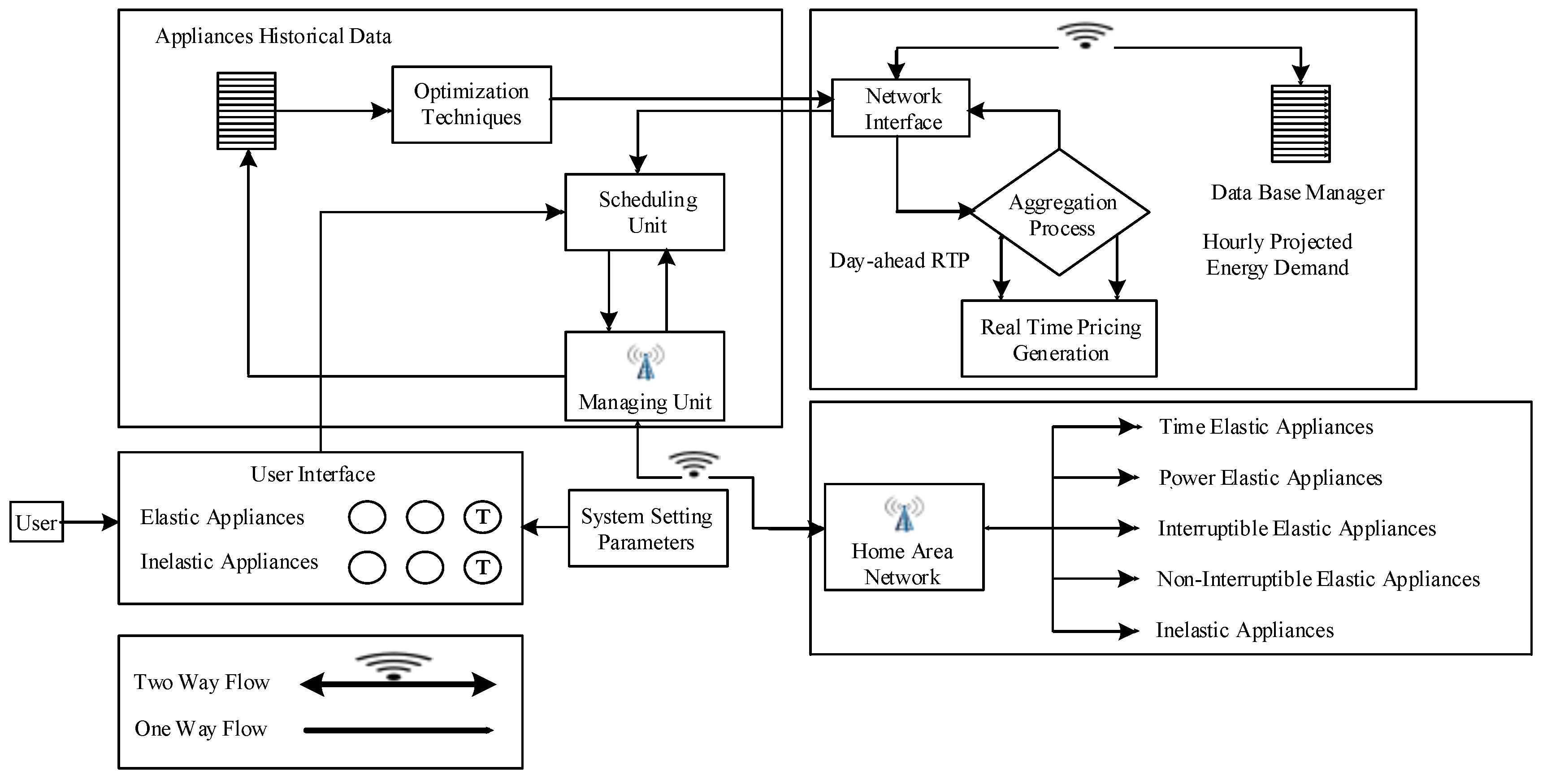The ECSU is connected to the utility company through the network interface such as local area network as shown in Figure 2. The ECSU receives control parameters setting from users through the user interface and pricing information from the utility to schedule the household appliance’s consumption behaviour.

Each user inputs control parameters such as starting time, ending time and length of operation time, etc., through the user interface to the scheduling unit. The scheduling unit receives price information from utility, and forwards control parameters and price information to managing units. Using historical data and data received from scheduling unit; the managing unit schedules appliances consumption behavior using optimization techniques. Finally, ECSU exchanges the schedule with the utility to optimally control the consumer’s consumption behavior as shown in Figure 3.

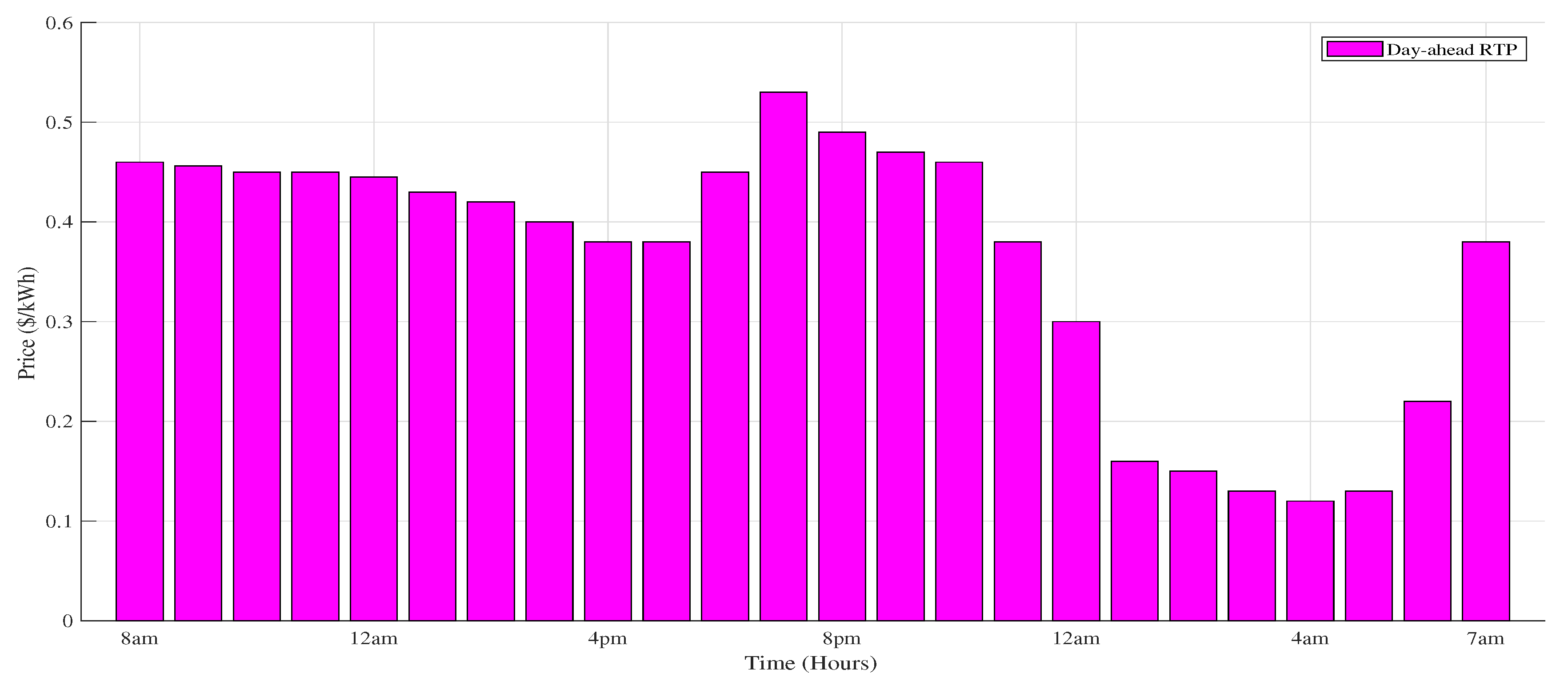
The scheduling time horizon is divided into T time slots, where $T=\{1,2,3,\dots \dots .,T\}$. The utility generates day-ahead RTP signal. This division and day-ahead RTP is based on the behavior of consumers and their demand patterns, such as on-peak time slots, off-peak time slots, and mid-peak time slots.

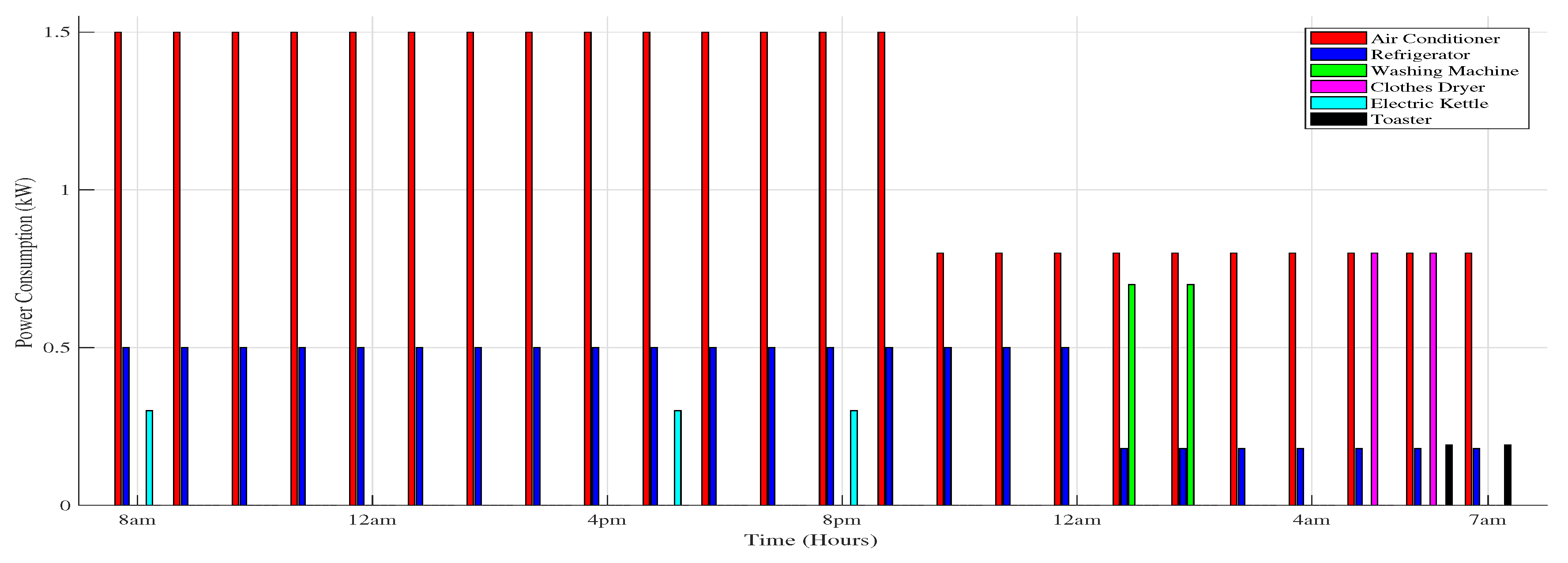
The load demand is classified into two types: elastic load and inelastic load. Moreover, the elastic loads is further classified into two categories: time elastic appliances and power elastic appliances. Each time elastic appliance can either be interruptible or non-interruptible. The operation of interruptible appliances can be delayed, interrupted and adjusted or shifted to the time slots other than on-peak time slots, while, for non-interruptible appliances, it is only possible to delay its operation, when needed. On the other hand, there is the inelastic load, having an inflexible price nature. The detailed description of appliances is as follows.

Let the set of appliances are denoted by: $A=\{A_e^t,A_e^p\}$, such that, $A_e^t=\{A_{te}^n,A_{te}^{in}\}$. $A_e^t$ is the set of time elastic appliances and $A_e^p$ is the set of power elastic appliances. For each appliance i, the current position, $S_t^i=(r_t^n,w_t^n)$ and the position at the next time slot, $S_{t+1}^i$ is defined. In the time elastic appliances, the operation of interruptible appliances can be adjusted and interrupted, if necessary. The initial position and the position at next time slot for interruptible appliances can be modeled as shown below in Equations (15) and (16):

$$S_t^i=\{T_s^o,\beta -\alpha +T_s^o+1\},$$

(15)

$$S_{t+1}^i=\left\{\begin{array}{c}{r}_t^n,w_t^n-1\mathrm{if}{X}_t=0,w_t^n\ge 1,\hfill \\ r_t^n-1,w_t^n\mathrm{if}{X}_t=1,r_t^n\ge 1.\hfill \end{array}\right.$$

(16)

In time elastic appliances, the non-interruptible appliances can only be delayed on the user requirement, as discussed above. The initial position and position at next time slot for non-interruptible appliances are modeled as in Equations (17) and (18):

$$S_t^i=\{T_s^o,\beta -\alpha +T_s^o+1\},$$

(17)

$$S_{t+1}^i=\left\{\begin{array}{c}{r}_t^n,w_t^n-1\mathrm{if}{X}_t=0,w_t^n\ge 1,\hfill \\ r_t^n-1,w_t^n\mathrm{if}{X}_t=1,r_t^n\ge 1.\hfill \end{array}\right.$$

(18)

The power elastic appliances have elasticity in their power rating, and tolerate flexibility in their operation time. The position of power elastic appliances at the next time slot is modeled as in Equation (19):

$$S_{t+1}^i=\left\{\begin{array}{c}{p}_{max}^i\mathrm{if}{X}_t=1,8\mathrm{a}.\mathrm{m}.\le \mathrm{t}<9\mathrm{p}.\mathrm{m}.,\hfill \\ p_{min}^i\mathrm{if}{X}_t=1,10\mathrm{p}.\mathrm{m}.\le \mathrm{t}<7\mathrm{a}.\mathrm{m}.\hfill \end{array}\right.$$

(19)

The inelastic appliances start operation immediately and need to be power-on at all times during the day. The initial position and the position at next time slots are given as in Equations (20) and (21):

$$S_t^i=\left(T_{s,}^{o}0\right),$$

(20)

$$S_{t+1}^i=\left\{\begin{array}{c}{r}_t^n,0\mathrm{if}{X}_t=1,r_t^n\ge 1,\hfill \\ 0,0\mathrm{otherwise}.\hfill \end{array}\right.$$

(21)

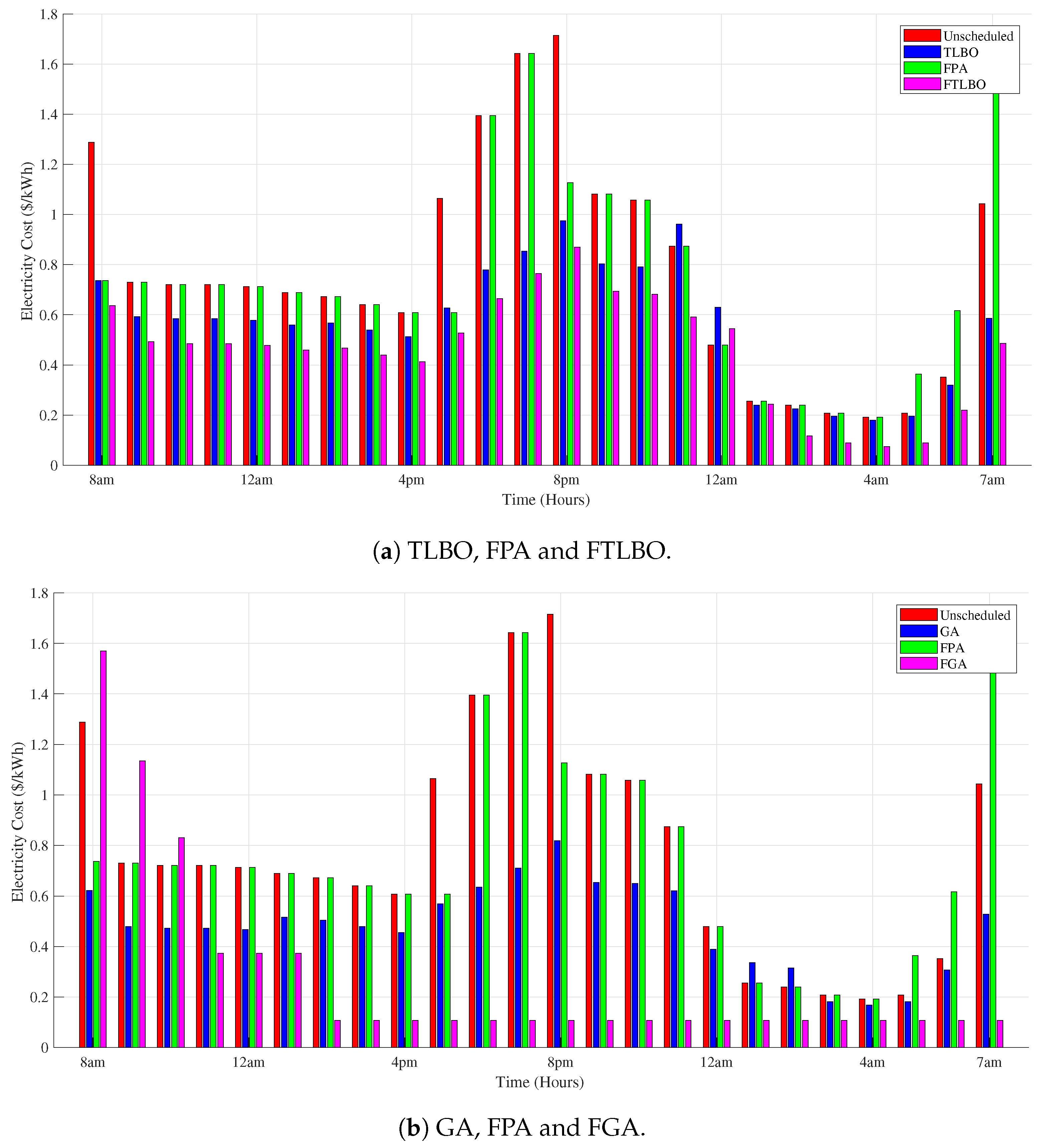
Among the various pricing schemes discussed below, the RTP scheme is chosen because it has more flexibility for appliances scheduling as compared to the ToU tariff, CPP and CPR. To avoid the building of peaks during off-peak hours, the combined RTP and inclined block rate (IBR) pricing scheme are considered. We assume that the utility has no control over the consumer’s consumption and it may only influence the load by providing price flexibility. Load synchronization and building of peaks during off-peak hours can be avoided by adopting combined RTP with IBRs, where the marginal price has a direct relationship with the load. This combined pricing scheme encourages the consumer to shift the load from on-peak to off-peak hours in order to reduce cost and PAR. Using this combined pricing scheme, electricity price depends on time and also on total load. Let $\rho \left(L^t\right)$ indicate the electricity price at time slot t, as a function of consumer’s consumption at that time slot as shown using Equation (22):

$$\rho \left(L^t\right)=\left\{\begin{array}{c}{R}_t\mathrm{if}0<L^t\le L_{th},\hfill \\ b_t\mathrm{if}{L}^t\ge L_{th},\hfill \end{array}\right.$$

(22)

where $R_t$ is the electricity price, when the total consumption is less than the threshold of IBRs at time slot t, and $b_t$ is the electricity price at time slot t, when the total consumption exceeds the threshold of IBRs.

5. Optimization Techniques

Many mathematical and heuristics techniques have been used for appliances scheduling. The main objectives of using these techniques for optimization are the reduction of electricity bill, PAR and energy balancing for demand and supply. In addition, optimizing grid stability, UC and to bring power quality are some other objectives. One of the key features of heuristics techniques is the low execution and computation time. These techniques provide a feasible solution to the problem. The details of these techniques used in this work are provided below. Algorithms are described in Algorithm 1–Algorithm 4.

5.1. Existing Optimization Techniques

This section provides a brief discussion of GA, TLBO, BAT and a flower pollination algorithm (FPA).

5.1.1. GA

GA is an adaptive heuristic search algorithm that is based on the evolutionary ideas of genetics and natural selection. GA is used to solve optimization problems and represents an intelligent exploitation of a random search. It tends to transfer random search towards a better performance region within the search space. GA performs a search in a multi-model state-space, large state-space or n-dimensional surface and offers significant benefits over many other typical optimization techniques. GA parameters for optimal results are given below in

Table 2. GA parameters.

Parameters	Value
Number of iterations	500
Population size	200
$P_m$	0.1
$P_c$	0.9
n	11

. To solve a problem over consecutive generations, GA simulates the survival of the fittest among individuals [40].

Each individual has a set of characteristics called chromosome or genotype bearing genes, which can be altered or mutated to produce individuals with best characteristics than the parents. Generally, GA candidate solutions are represented as a binary string of 0’s and 1’s; however, other encodings are also possible [41]. The gene pattern of chromosome represents the ON/OFF state of appliances and the length of chromosome represents the number of appliances. Once the population is created, i.e., the ON/OFF states of appliances are initialized in a particular time slot. The fitness of each candidate solution is calculated according to the objective function defined for the optimization problem. After evaluating the fitness of each candidate solution, crossover and mutation process is applied to produce offsprings known as a new population which is better than the parents.

5.1.2. TLBO

This algorithm was originally proposed by [42]. TLBO is computationally very efficient because its parameters do not require any tuning. TLBO consists of a teacher and a student. The teacher is considered the most knowledgeable person. The teacher shares its knowledge with the students to improve their output or performance. The quality of the student knowledge or performance can be found by evaluating their grades. Moreover, the students also improve their knowledge by discussion, which ultimately improves their performance [43]. TLBO is a population-based algorithm inspired by the teaching and learning environment of the classroom. TLBO consists of two phases: teacher phase and student phase. In the first phase, a teacher is chosen as the best solution for the population and the remaining population is considered as students. To raise the level of the students, the teacher gave his knowledge to the students for changing the average value of the students knowledge. The mean difference between the teacher and the student’s knowledge in a specific subject can be given by the following Equations (23)–(25):

$$M{D}_i=r_i(Mea{n}_{new}-T_{factor}\times Mea{n}_i),$$

(23)

$$T_{factor}=round[1+rand(0,1)\left\{2-1\right\}],$$

(24)

$$X_{new,i}=X_{old,i}+M{D}_i,$$

(25)

where $M{D}_i$ presents the mean difference of knowledge between the teacher and students, $Mea{n}_{new}$ presents the outcome of the best learner in particular subject. $r_i$ indicates the random number between 0 and 1. $T_{factor}$ presents a teaching factor and its value can be 1 or 2 and is a heuristic step decided randomly with equal probability. The updated value of $X_{new,i}$ is chosen in the population if it is better than the $X_{old,i}$.

In the student phase, the students interact with each other and the student with less knowledge learns from the student with more knowledge. Two students, i.e., s1 and s2 are randomly selected from the initial population such that $X_{total-s1,i}\ne X_{total-s1,i}$. However, the optimization problem can be given as below using Equations (26) and (27):

$$\begin{array}{cc}{X}_{fnew,s1,i}=X_{new,s1,i}+r_i(X_{new,s1,i}+X_{new,s2,i}),\hfill & \\ & \hfill if{X}_{new,total-s1,i}\le X_{new,total-s1,i},\end{array}$$

(26)

$$\begin{array}{cc}{X}_{fnew,s1,i}=X_{new,s1,i}+r_i(X_{new,s2,i}+X_{new,s1,i}),\hfill & \\ & \hfill if{X}_{new,total-s2,i}\le X_{new,total-s2,i}.\end{array}$$

(27)

The solution $X_{fnew,s1,i}$ is selected, if its results are better than the existing one; otherwise, it is discarded. These selected values are given as input to the teacher phase in the next iteration. This process repeats until the termination criteria are reached.

5.1.3. BAT

The BAT is a meta-heuristic algorithm used for global optimization. It was developed by Xin-She Yang in 2010 and inspired by the echolocation behavior of microbats. The varying pulse rates of emission and loudness of the bat algorithm helps in finding the particular location via sound waves. The idea of the echolocation of microbats can be explained as follows: each virtual bat flies randomly with a velocity $v_i$ at position (solution) $x_i$. The frequency and loudness of the bat vary continuously. It changes frequency, pulse emission rate and loudness, as it searches and finds its prey via local random walk. Selection of the best prey continues until certain stopping conditions are met. To control the dynamic behavior of a swarm of bats, essentially a frequency-tuning technique is used. In the BAT algorithm, tuning algorithm-dependent parameters are very essential for controlling the balance between exploration and exploitation [44].

5.1.4. FPA

Flower pollination is an interesting process in the natural world. FPA is inspired by the pollination process of flowers in flowering plants. The aim of the flower pollination is the existence of the fittest and the optimal reproduction of plants. This is actually an optimization process of the flowering plants. There are two types of pollination: biotic and abiotic. Biotic pollination takes place in 90% of the flowering plants. Insects and animals act as pollinators which transfer pollen grain in flowering plants. Pollinators are also called pollen vectors, which are very diverse in nature. An estimated 200,000 of pollinators exist such as animals, birds, bats and insects. Cross and biotic pollination is a global pollination process. Due to random flights, the pollinators carry pollens to various places. Local pollination is considered as abiotic and self-pollination process. A switch probability p ∈ [0, 1] controls the global and local pollination process. Due to the wind and physical proximity, local pollination has p, as a fraction of the overall pollination process.

5.2. Proposed Optimization Techniques

A brief overview of the proposed techniques: GTLBO, FBAT, FTLBO and FGA are provided in this section. In this work, basically four heuristic algorithms are used, i.e., GA, TLBO, FPA and BAT. Based on these algorithms, four hybrid algorithms, i.e., GTLBO, FTLBO, FBAT and FGA are proposed.

5.2.1. GTLBO

GTLBO is a hybrid technique that is made by combining the parameters of GA and TLBO. TLBO performs better in searching of an optimal solution as well as in exploitation mode, i.e., finding the best solution in local search space; however, TLBO performs very poorly in exploration mode. It is designed for a fast and local search, while, in a global search, the searching time is too long. Thus, there must be a balance between exploration and exploitation to find the best solution. GA performs best in exploration mode (global search) in addition to having a good convergence rate. GA has the efficiency to search in large spaces without trapping in local optima. In designing the algorithm, exploration and exploitation modes are two important aspects that are taken into consideration. To overcome the imbalance between exploration and exploitation mode of TLBO, a hybrid technique is proposed by applying the crossover and mutation operator of GA to TLBO. Hybrid techniques, initially, works as TLBO. After updating the population in learner mode, crossover and mutation are applied. Then, new vectors are added to the population to calculate fitness. The process continues until termination is reached.

The hybrid technique takes the advantage of both exploration and exploitation mode of TLBO and GA. The proposed technique is able to maintain a balance between local and global search by applying crossover and mutation operator of GA to TLBO as well as having a better convergence rate.

Algorithm 1 GTLBO

1: Initialize number of students, number of subjects, i.e., variables, d, termination criteria 2: Calculate the mean of each variable or subjects 3: Find the best solution and best variable value 4: while Stopping condition not met do 5:     for each learner X, of the class do 6:         Teaching phase = round (1 + rand(0, I)) 7:         for j = 1 : d do 8:            $New{X}_{ij}$ = $X_{ij}$ + rand(0, 1) * (teacher(j)- 9:            teaching phase ∗ mean(j) 10:         end for 11:         Accept $new{X}_i$ if $f\left(new{X}_i\right)$ is better than $f\left(X_i\right)$ 12:     end for 13:     for each learner $X_i$ of the class do 14:         Randomly select one learner $X_k$, such that $i\ne k$ 15:         if $\mathbf{then}f\left(X_i\right)$ better $f\left(X_k\right)$ 16:            for j = 1 : d do 17:                $new{X}_{ij}=X_{ij}+rand(0,1)*(X_{ij}-X_{kj})$ 18:            end for 19:         else 20:            for j = 1 : d do 21:                $new{X}_{ij}$ = $X_{ij}$ + rand(0, 1) * $(X_{kj}-X_{ij})$ 22:            end for 23:         end if 24:         Perform GA crossover operation on $new{X}_{ij}$ 25:         Perform mutation operation on the new population; 26:         Use an objective function to take a new population as 27:         input after crossover and mutation; 28:         if off-spring is better than previous population then 29:            Accept new population 30:         else 31:            Move to the next iteration and repeat the 32:            process; 33:            Until termination criteria reached or first 34:            learner phase end; 35:         end if 36:         From learning phase one accept results and run 37:         second learning phase; 38:         Perform crossover and mutation operation and run 39:         objective function; 40:         Repeat the process for each learning phase; 41:         Accept $new{X}_i$ if $f\left(new{X}_i\right)$ is better than $f\left(X_i\right)$ 42:     end for 43:     Update the teacher and the mean 44: end while

5.2.2. FBAT

FBAT is a hybrid algorithm made of FPA and BAT. Initially, the population is randomly generated for finding initial best solution using objective function. After evaluating the population; the BAT velocity, frequency and position steps are replaced by the main steps of FPA, i.e., local pollination is started and random flowers are found in the neighborhood. Then new solutions are evaluated by checking their fitnesses, if fitness improves, i.e., better solutions are found, then update the existing solutions and update the current global best solution. In the same manner, update the search space accordingly. The hybrid technique, i.e., FBAT performance is better than FPA and BAT in terms of cost, PAR and discomfort reduction as shown in

Table 3. Comparison of heuristic techniques (reduced).

Heuristic Technique	Daily Cost (%)	Daily Discomfort (%)	Peak Power Consumption (%)	PAR (%)
GA	37.95	7.56	9.87	9.87
TLBO	26.74	3.33	12.96e	12.96
FPA	3.87	30.91	38.27	5.55
BAT	12.32	48.36	2.46	2.46
Existing aggregate	20.22	22.54	15.89	7.71
GTLBO	39.17	44.45	32.09	32.09
FTLBO	40.75	33.38	45.06	45.06
FBAT	25.23	22.18	27.16	27.16
FGA	64.49	12.72	33.95	33.95
Proposed aggregate	42.41	28.1825	34.565	34.565

, and simulation section. The daily cost reduced by FPA, BAT and FBAT are 3.87%, 12.32% and 25.23%, respectively. Hence, the daily cost reduction by FBAT is more than FPA and BAT algorithms. In addition, the daily discomfort and PAR reduction by FPA and BAT are 30.91%, 5.55% and 48.36%, 2.46%, respectively, while 22.18%, and 27.16% by FBAT. As Table 3, shows that PAR and daily cost is reduced by FBAT as compared to FPA and BAT; however, the daily discomfort is reduced less by FBAT as compared to FPA and BAT due to trade-off between cost and daily discomfort.

Algorithm 2 FBAT

1: Population size, number of appliances d, frequency q, velocity v, no of iteration, probability switch, maximum and minimum frequency; 2: Initialize the population/solutions; 3: Generate population; 4: Find the initial best solution; 5: Initialize the best solution 6: Declare coefficients of objective function 7: Evaluate the population 8: FPA parameters replaces the BAT frequency, velocity and position calculation method; 9: forj = 1 : Niteration do 10:     for i = 1 : n do 11:         Local pollination will start 12:         if $rand>p1$, then 13:             L = Levy (d); 14:             dS = L.*(Sol(i,:)-gbest); 15:             Snew (i,:) = Sol (i,:) + dS; 16:         else 17:             Epsilon = rand; 18:             Find random flowers in the neighbourhood 19:             JK = randperm (n); 20:             Snew (i,:) = Snew (i,:) + epsilon * (Snew 21:             (JK(1),:) - Snew (JK(2),:)); 22:             Check if the simple limits/bounds are OK 23:             Sol1 (i,:) = simplebounds (Sol1 (i,:) , Lb, Ub); 24:             Improvise a new harmony vector 25:         end if 26:         Evaluate new solutions by checking their fitnesses 27:         Fnew = Fun (Snew (i,:)); 28:         If fitness improves (better solutions found), update 29:         the population 30:         if $Fnew<=F\left(i\right)$, then 31:             Sol (i,:) = Snew (i,:); 32:             F1 (i) = Fnew; 33:         end if 34:         Update the current global best 35:         if $Fnew<=fmin$, then 36:             gbest = Snew (i,:); 37:             fmin = Fnew; 38:         end if 39:         best; 40:         $fmin$; 41:     end for 42: end for

Algorithm 3 FTLBO

1: Initialize number of students, number of subjects, i.e., variables, d, termination criteria, population size, probability switch; 2: Calculate the mean of each variable or subjects; 3: Find the best solution and best variable value; 4: while Stopping condition not met do 5:     Teaching phase, generate new population and accept 6:     new if better than previous; 7:     for each learner $X_i$ of the class do 8:         Randomly select one learner $X_k$, such that $i\ne k$; 9:         FPA parameters replaces the TLBO teaching and 10:        learning phases; 11:        for j = 1 : Niteration do 12:            for i = 1 : n do 13:                Local pollination will start; 14:                if $rand>p1$ then, 15:                     L = Levy (d); 16:                     dS = L.* (Sol (i,:) - gbest); 17:                     Snew (i,:) = Sol (i,:) + dS; 18:                else 19:                     Epsilon = rand; 20:                     Find random flowers in the neighbour 21:                     hood; 22:                     JK = randperm (n); 23:                     Snew (i,:) = Snew (i,:) + epsilon * 24:                     (Snew (JK(1) ,:) - Snew (JK(2),:)); 25:                     Check if the simple limits/bounds are 26:                     OK; 27:                     Sol1 (i,:) = simplebounds (Sol1 (i,:), 28:                     Lb, Ub); 29:                     Improvise a new harmony vector; 30:                end if 31:                Evaluate new solutions by checking their 32:                fitnesses; 33:                Fnew = Fun (Snew (i,:)); 34:                If fitness improves (better solutions found), 35:                update the new population; 36:                if $Fnew<=F\left(i\right))$ then, 37:                     Sol (i,:) = Snew (i,:); 38:                     F1(i) = Fnew; 39:                end if 40:                Update the current global best; 41:                if $Fnew<=fmin$ then, 42:                     gbest = Snew (i,:); 43:                     fmin = Fnew; 44:                end if 45:                best; 46:                $fmin$; 47:            end for 48:         end for 49:     end for 50:     Update the teacher and the mean value; 51: end while

Algorithm 4 FGA

1: Initialize population, population size, number of iteration, crossover and mutation rate, number of appliances, probability switch; 2: Generate an initial random population; 3: while Stopping condition not met do 4:     Iteration ≤ Maximum iteration; 5:     Iteration = iteration + 1; 6:     Define objective function; 7:     Calculate the fitness of each individual via objective 8:     function; 9:     Select the individuals which are fittest among the 10:    population generated; 11:    FPA parameters replaces the TLBO teaching and 12:    learning phases; 13:    for j = 1 : Niteration do 14:         for i = 1 : n do 15:            Local pollination will start; 16:            if $rand>p1$ then, 17:                 L = Levy (d); 18:                 dS = L.* (Sol (i,:) - gbest); 19:                 Snew (i,:) = Sol (i,:) + dS; 20:            else 21:                 Epsilon = rand; 22:                 Find random flowers in the neighbour 23:                 hood; 24:                 JK = randperm (n); 25:                 Snew (i,:) = Snew (i,:) + epsilon * 26:                 (Snew (JK(1) ,:) - Snew (JK(2),:)); 27:                 Check if the simple limits/bounds are 28:                 OK; 29:                 Sol (i,:) = simplebounds (Sol (i,:), 30:                 Lb, Ub); 31:                 Improvise a new harmony vector; 32:            end if 33:            Evaluate new solutions by checking their 34:            fitnesses; 35:            Fnew = Fun (Snew (i,:)); 36:            If fitness improves (better solutions found), 37:            update the new population; 38:            if $Fnew<=F\left(i\right))$ then, 39:                 Sol (i,:) = Snew (i,:); 40:                 F1(i) = Fnew; 41:            end if 42:            Update the current global best; 43:            if $Fnew<=fmin$ then, 44:                 gbest = Snew (i,:); 45:                 $fmin=Fnew$; 46:            end if 47:            best; 48:            $fmin$; 49:         end for 50:     end for 51:     Desired population, which are selected after FPA 52:     pollination process; 53: end while

5.2.3. FTLBO

FTLBO is the hybrid of FPA and TLBO techniques. FTLBO performance is better than FPA and TLBO as shown in simulation and Table 3. The daily cost reduction, daily discomfort and PAR by FPA, TLBO and FTLBO are 3.87%, 30.91%, 5.55%, 26.74%, 3.33%, 12.96%, and 40.75%, 33.38%, 45.06%, respectively. Hence, the daily cost and PAR reduction by FTLBO is more as compared to FPA and TLBO. In case of daily discomfort, the FTLBO performance is better than FPA and TLBO. The FTLBO reduced the daily discomfort very little as compared to FPA because there is trade-off between cost and discomfort. As the cost by FPA is reduced very little, the discomfort is increased by 30.91%. By making the FTLBO, all the steps of TLBO, i.e., population initialization and random generation, evaluate the population or solutions, find best fitness and select for the next generation, are followed. However, the two main steps of TLBO, i.e., the teaching and learning phase are replaced with the main steps of FPA, i.e., after starting the local pollination, random flowers are searched and found in the neighborhood of FPA. The new solutions are found and their fitness values are checked to compute the best solution. The best solutions found are chosen for the next generation based on the global best solutions.

5.2.4. FGA

FGA is made by FPA and GA. In FGA, all the steps of GA are followed except the two main steps, i.e., crossover and mutation, which generate new solutions in each iteration. The steps are replaced by the FPA pollination process as already discussed in section GTLBO and FTLBO.

6. Simulations and Discussion

In this section, simulation results and performance of the proposed algorithms are discussed. Load scheduling is performed under day-ahead pricing (DAP) as shown in Figure 4, taken from the daily report of FERC [38]. Total time horizon is 24 h, whereas hourly time slots are taken for scheduling of appliances. The problem is formulated as an optimization problem with the objectives to minimize electricity consumption cost and user discomfort. The problem is solved using four existing optimization techniques: GA, TLBO, FPA, BAT and four proposed hybrid techniques: GTLBO, FTLBO, FBAT and FGA. Results show that power flexible appliances operate at low power, where the prices are high, while time flexible appliances delay their operation onto off-peak hours. A comparison of above mentioned techniques is provided in Table 3. A detailed discussion of performance parameters is provided as below:

6.1. Power Consumption

Power consumption depends on power rating and the length of the operation time of appliances. Minimizing power consumption during on-peak hours minimizes the cost; however, user discomfort increases. Figure 4 illustrates that 6:00 p.m.–10:00 p.m. is on-peak hours, whereas 1:00 a.m.–6:00 a.m. is off-peak hours. To achieve the objectives, power consumption must be minimized at on-peak hours and maximized at off-peak hours. The hourly power consumption of all appliances using GA, TLBO, FPA, BAT and the hybrid techniques are shown in Figure 5.

As it can be seen in Figure 6 and Figure 7, GA, TLBO, FPA, BAT and the hybrid techniques: GTLBO, FTLBO, FBAT and FGA have peak hourly power consumption of 2.10 kW, 2.6 kW, 3.1 kW, 4.7 kW, 2.3 kW, 2.2 kW, 4.7 kW and 5.5 kW, respectively, whereas FGA has the peak hourly power consumption of 2.42 kW that is highest among all the techniques. As it is depicted from the FGA schedule provided in Figure 6b, the washing machine is scheduled to operate at 1:00 a.m., where two power flexible appliances are already in operation; this resulted in peak creation. Results demonstrate that FTLBO outperforms all other techniques in terms of achieving minimum peak power consumption as shown in Figure 6a and Table 3.

The power consumption of each appliance is shown in Figure 5. Figure 5 illustrates that an air conditioner consumes 1.5 kW from 8:00 a.m. to 8:00 p.m. and 0.8 kW from 9:00 p.m. to 7:00 a.m. The refrigerator uses 0.5 kW from 8:00 a.m.–12:00 a.m. and 0.3 kW from 1:00 a.m.–7:00 a.m. The washing machine is ON from 1:00 a.m.–2:00 a.m. and consumes 0.7 kW power. From 5:00 a.m.–6:00 a.m. the clothes dryer operates and consumes 0.8 kW power. Electric kettle consumes 0.3 kW at 8:00 a.m., 5:00 p.m. and 8:00 p.m. Electric toaster runs for two hours, i.e., 6:00 a.m.–7:00 a.m. and consumes 0.2 kW power.

Figure 6 shows the hourly power consumption of appliances in unscheduled case for TLBO, FPA, GA, FPA and their hybrid: FTLBO and FGA respectively. The peak unscheduled power consumption is at 8:00 a.m., i.e., 3.5 kW, while low peak power consumption is 1.6 kW during the rest of the hours. The peak power consumption by TLBO is 2.6 kW at 11:00 p.m. and power consumption is low for the rest of the hours, i.e., 1.3 kW. At 7:00 a.m., FPA has the highest power consumption, i.e., 3.9 kW and 1.6 kW for the remaining hours. The FTLBO has peak power consumption from 12:00 a.m. and 1:00 a.m., i.e., 2.2 kW and below 1.5 kW during the rest of the hours. GA power consumption from 1:00 a.m.–2:00 a.m. is 2.2 kW and the lowest in the other time slots as shown in Figure 6a, while 8:00 a.m.–10 a.m. shows the peak power consumption by FGA. The power consumption by FTLBO and FGA is less than FPA; however, it is equal to TLBO and more than GA as shown in Figure 6.

Figure 7 shows the hourly power consumption by unscheduled case, GA, TLBO, BAT, FPA and their hybrid, i.e., GTLBO and FBAT, respectively. The peak power in the unscheduled case is 3.5 kW at 8:00 p.m. and the lowest power consumption is 1.6 kW at many other hours as shown in Figure 7a,b. Peak power consumption by GA from 1:00 a.m.–2 a.m. is 2.2 kW and the lowest power consumption is 1.1 kW. In conclusion, TLBO shows the peak power consumption at 11:00 p.m., i.e., 2.6 kW and the lowest from 9:00 a.m. to 4:00 p.m., while GTLBO shows the peak power consumption of 2.3 kW at 1:00 a.m. The power consumption by BAT is highest at 1:00 a.m., i.e., 3.5 kW and the lowest is 1.7 kW for the rest of the hours. The peak power consumption by FBAT is 3.5 kW at 7:00 a.m., while for the rest of the hours, the power consumption is 1.6 kW.

6.2. Electricity Consumption Cost

Cost minimization is one of the primary objectives of power scheduling where appliances are scheduled to minimize user’s electricity bill. However, the user discomfort is increasing with cost minimization due to trade-off between cost and discomfort. Daily consumption cost after scheduling appliances by all optimization techniques is given in Figure 8. The results show that GA and FGA have lowest cost in all the times slots. The reason for this much cost reduction using GA and FGA is clear from power consumption pattern illustrated in Figure 6, which shows that hourly power consumption of GA and FGA is minimum as compared to TLBO, FPA, BAT and the hybrid algorithms.

Figure 7 and Figure 8 show the hourly electricity cost of appliances. The unscheduled cost is high from 7:00 a.m.–10 a.m. and 5:00 p.m.–8 p.m., which is about $1/kW. The cost by TLBO from 7:00 p.m.–11 p.m. is high, nearly $0.84/kW and has the lowest cost from 1:00 a.m.–6:00 a.m. This is due to the off-peak hours. The cost by FPA is high from 6:00 p.m.–11:00 p.m. and 7:00 a.m., while the lowest cost is from 1:00 a.m.–6:00 a.m. due to off-peak hours. Similar to the case with FTLBO, however, it reduces the cost as compared with the unscheduled case, TLBO and FPA for all hours. Hence, it shows that FTLBO is more cost efficient than TLBO and FPA. The cost by GA is higher at 8:00 a.m., 5:00 p.m.–11:00 p.m. and 7:00 a.m. due to on-peak hours and lowest from 1:00 a.m.–6:00 a.m. due to off-peak hours. The cost reduction by GA is more than the unscheduled case and FPA; however, it is not more than FGA. FGA has high and low cost from 6:00 p.m.–11:00 p.m., 5:00 a.m.–7:00 a.m. due to on-peak and off-peak hours, respectively, as shown in Figure 8b. The cost by FGA is high from 8:00 a.m.–10:00 a.m. and has the lowest cost at all other hours. FGA reduces cost more as compared to GA and FPA.

Figure 7 shows the hourly cost reduction by GA, TLBO, GTLBO, BAT, FPA and FBAT. The peak unscheduled cost is $0.9/kW at 8:00 p.m. and the lowest cost is $0.2/kW at 4:00 a.m. due to off-peak hours. GA, TLBO and GTLBO show high cost from 6:00 p.m.–11:00 p.m. and have the lowest cost from 1:00 a.m.–6:00 a.m. due to on-peak and off-peak hours. GTLBO is more efficient in cost reduction than GA and TLBO as shown in Figure 7b. Similarly, the cost reduction by BAT, FPA and FBAT is high from 6:00 p.m.–11:00 p.m. and 7:00 a.m. However, FBAT is more efficient in cost reduction than BAT and FPA, respectively, as shown in Figure 7b. Table 3 shows the daily cost reduction by FPA, BAT and FBAT, which are 3.87%, 12.32% and 25.23%, respectively. The hourly electricity cost of appliances is shown in Figure 9.

6.3. User Discomfort

Discomfort is caused due to two main reasons: delaying the operation of time-flexible appliances and the running of the appliances before its starting time from the time suitable for the consumers. From 6:00 p.m.–11:00 p.m. due to on-peak hours, user discomfort is maximum, whereas, from 12:00 a.m.–7:00 a.m. due to off-peak hours, user discomfort is minimum. Overall daily discomfort is depicted in Figure 10, which shows that BAT has the highest user discomfort, whereas GTLBO has minimum user discomfort. Comparison is made between parents and proposed hybrid techniques. Proposed techniques outperform their parents techniques considering user discomfort. Hourly discomfort caused by power-flexible appliances is illustrated in Figure 11. Figure 11a shows the hourly discomfort by GA, TLBO, GTLBO and in unscheduled case. The hourly discomfort by GA, TLBO and GTLBO is high during on-peak hours and a minimum at off-peak hours.

6.4. PAR

PAR provides a measure of how peak electricity consumption affects the system, particularly in efficiency and reliability. Figure 12 shows the scheduled and unscheduled PAR. The unscheduled PAR is 1.62, while the PAR by: GA, TLBO, GTLBO, BAT, FPA, FBAT, FTLBO and FGA are 1.46, 1.41, 1.58, 1.53, 1.18, 0.89 and 1.07, respectively. It can also be noted that the PAR by the proposed techniques: GTLBO, FTLBO, FBAT and FGA is 1.10, 0.89, 1.18, 1.07, respectively. This is less than their parent techniques. FTLBO has the minimum PAR among all of the techniques. High PAR in case of BAT resulted from peak power consumption as displayed in Figure 7. BAT has highest peak power consumption and it resulted in the high PAR.

6.5. Feasible Region for Electricity Cost and User Discomfort

Figure 13 shows the feasible region between electricity cost and user discomfort. The total cost for the unscheduled case is $16.62. Possible points are calculated using the minimum and maximum combinations of price and user discomfort. The main objective is to calculate the total maximum and minimum cost against maximum and minimum user discomfort. Reducing the overall energy consumption cost ultimately results in increasing user discomfort. To achieve the economic goals for a consumer, there is trade-off between electricity cost and user discomfort. Electricity price defined by the utility ranges from $11.30/kWh–$11.53/kWh. The minimum and maximum user discomfort are 1.6 and 3.8, respectively. Total covered area is obtained under points P1(0, 1269.8), P2(2.8334, 1072), P3(4.6191, 1036.8). To represent the feasible region, point P3 (4.6191, 1036.8) is plotted, which means that the electricity cost should be less than $11.53 to achieve the objective function of the minimal user discomfort. Hence, all three points P1, P2, P3 collectively form our feasible region for cost reduction by minimizing user discomfort. The feasible region using RTP is shown in Figure 13.

6.6. The Performance Parameters Trade-Off

Results show a trade-off between user discomfort and consumption cost. The feasible region for consumption cost provided in the system model section shows that maximum saving can be achieved by scheduling maximum load during off-peak hours. A relationship between user discomfort and cost is illustrated by feasible region depicted in Figure 13. User discomfort greatly affects consumption cost, i.e., by minimizing user discomfort, consumption cost increases with the increase of user discomfort, and the consumption cost decreases as shown in Table 3 and

Table 4. Performance trade-off.

Technique	Discomfort	Cost ($)	Technique	Discomfort	Cost ($)
GA	2.83	11.53	GTLBO	1.32	11.30
TLBO	2.50	13.61	FTLBO	1.58	11.01
FPA	1.76	17.86	FBAT	1.06	13.89
BAT	1.84	16.29	FGA	2.33	6.59

. Table 4 shows a performance trade-off between cost and user discomfort. GA reduces cost by 37.95%; however, daily discomfort reduces very little, i.e., 7.56%. Peak power consumption (PPC) and PAR is reduced to 9.87%. TLBO has cost reduction of 26.74% and the daily user discomfort is 3.33%, whereas PPC and PAR are reduced to 12.96%.

FPA has a cost reduction of 3.87%, and hence the decrease in discomfort is very high, i.e., 30.91%. This is high due to the consumption of load during peak hours. The decrease in PPC and PAR is 38.27% and 5.55%, respectively. BAT reduces cost up to 12.32%, while discomfort is up to 48.36%. The decrease in PPC and PAR is 2.46%. Cost reduction by GTLBO is 39.17% and discomfort is minimized up to 44.45%. The PPC and PAR are reduced by 32.09%. FTLBO reduces cost up to 40.75% and user discomfort is minimized to 33.38%, while PPC and PAR are reduced by 45.06%. FBAT reduces cost and user discomfort by 25.23% and 22.18%, while PPC and PAR are reduced by 27.16%. The cost reduction by FGA is very high, i.e., 64.49% due to which daily user discomfort is reduced, i.e., PPC and PAR are 33.95% reduced as shown in Table 3. Comparison provided in Table 3, which shows that hybrid techniques perform best in terms of achieving minimum cost, user discomfort, PPC and PAR.

7. Conclusions and Future Work

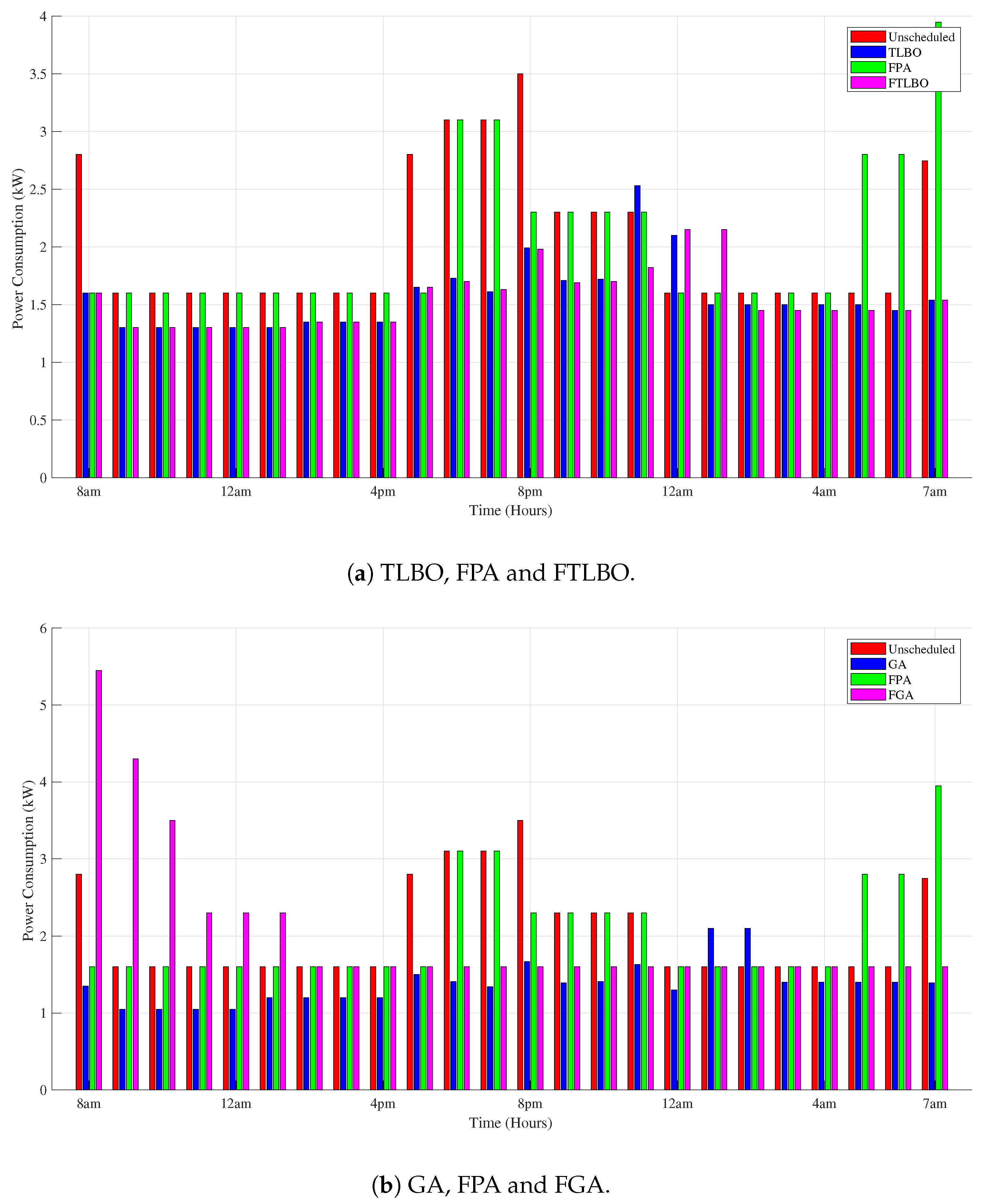
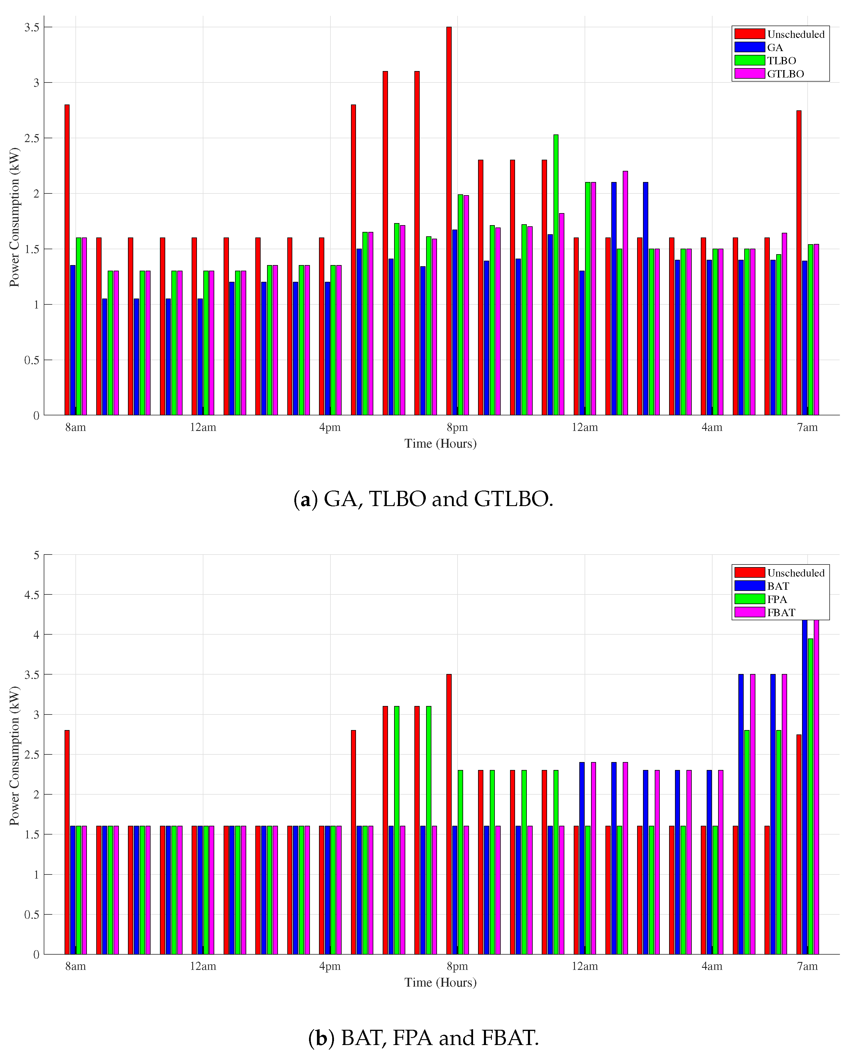
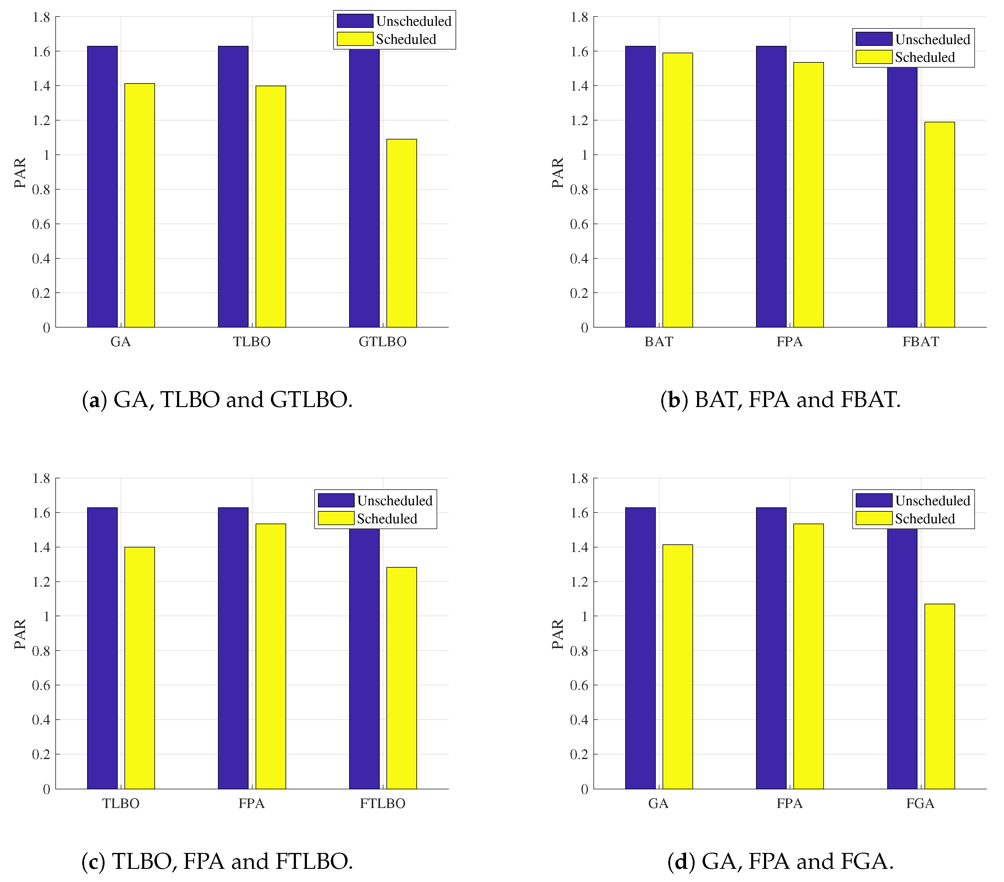
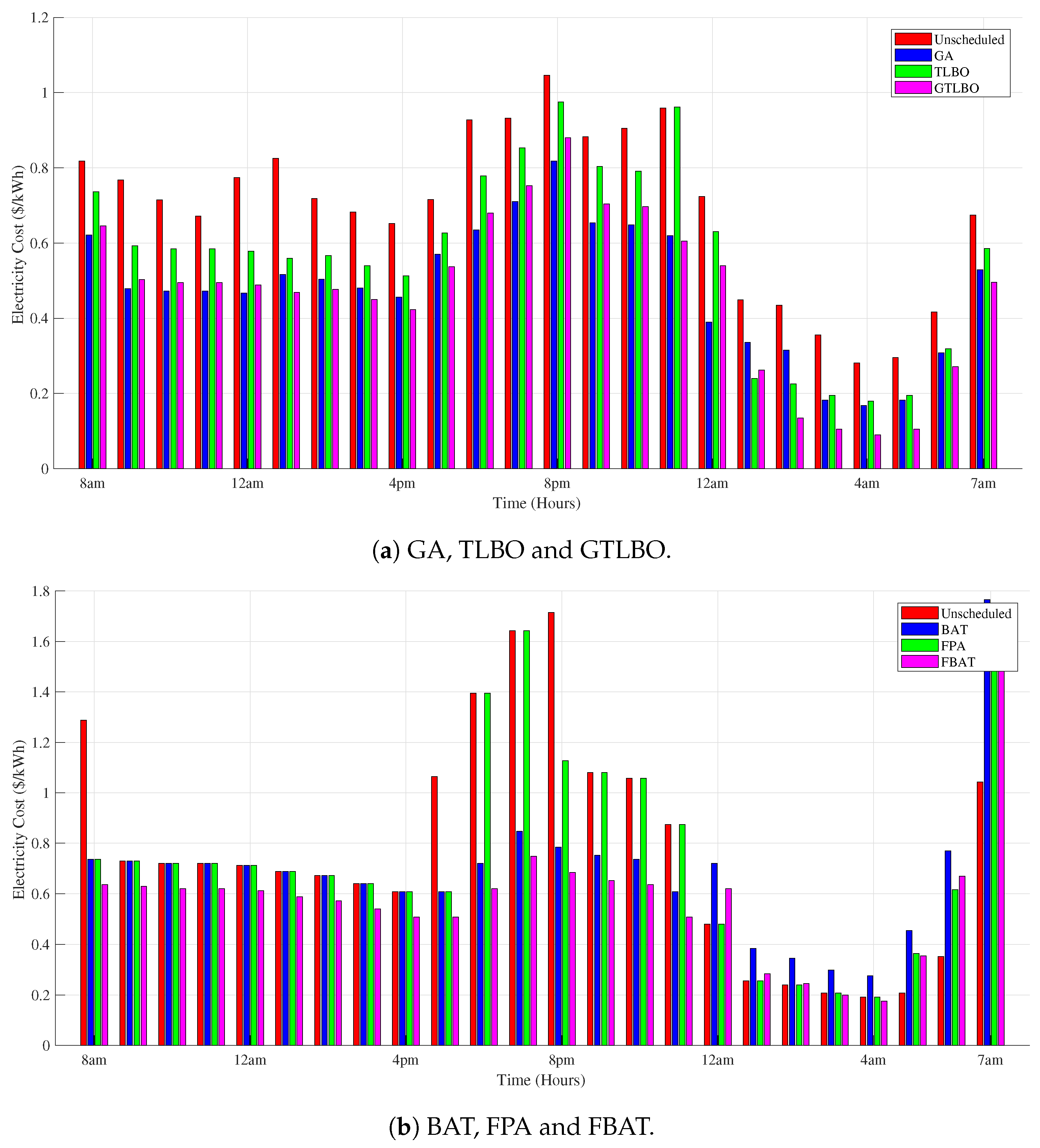
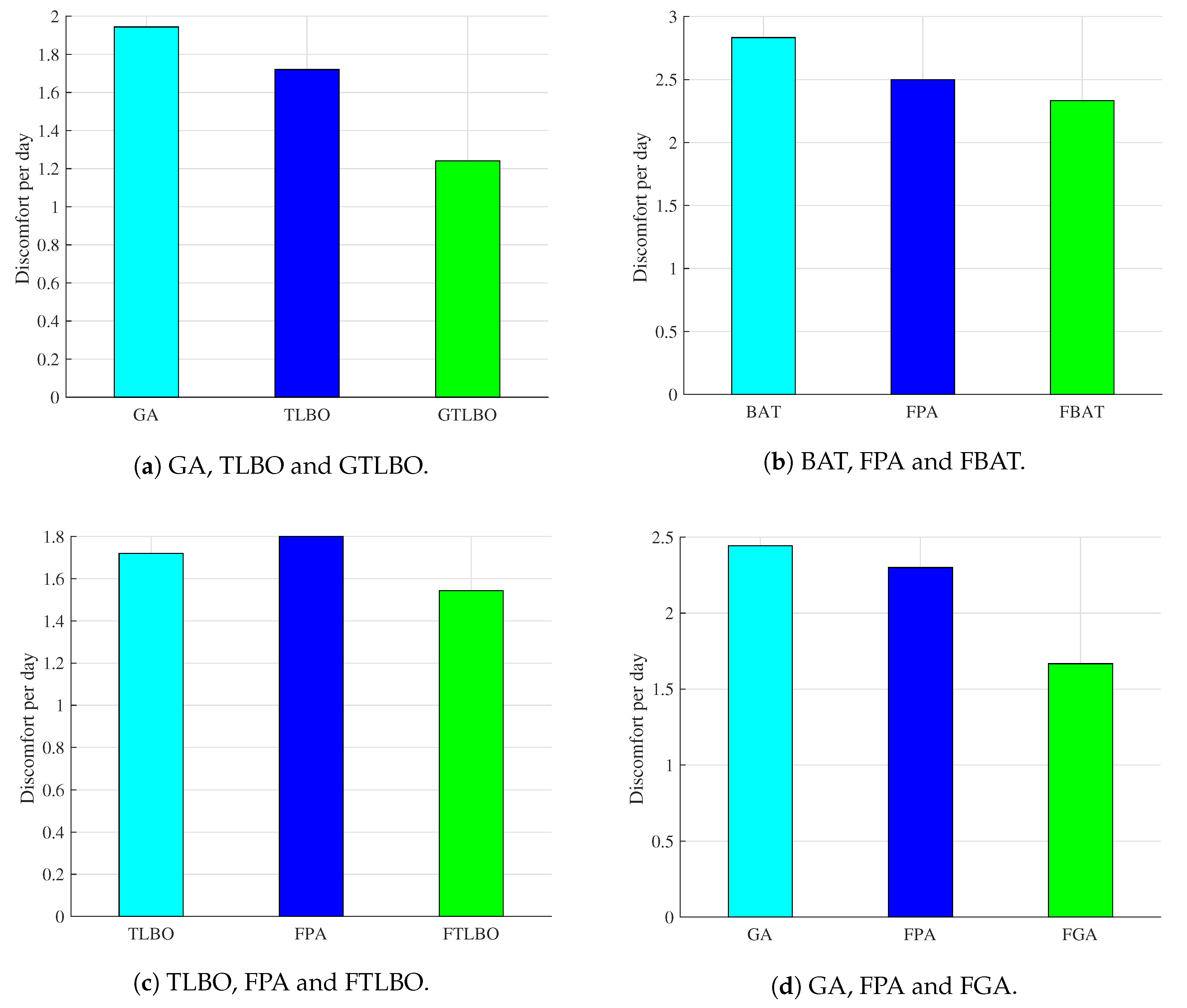
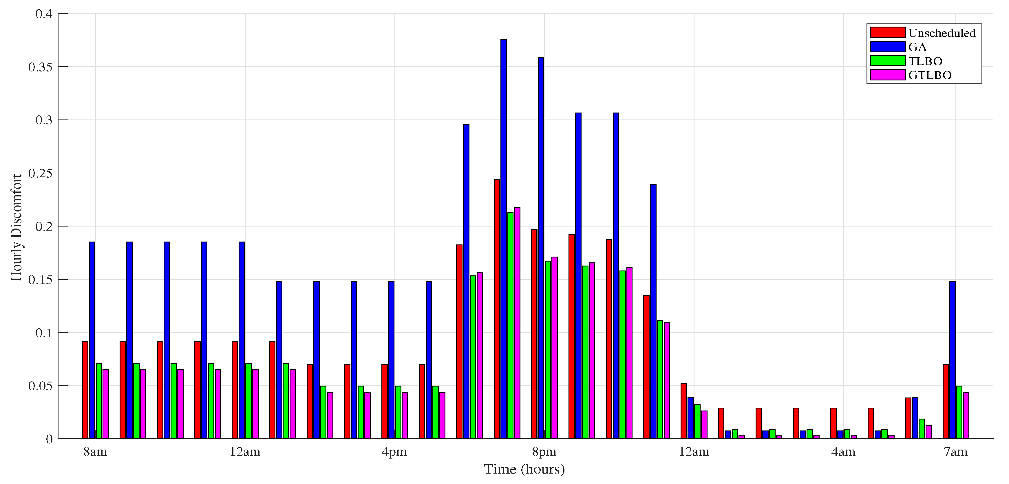
Residential load scheduling is a common method in DSM for smart homes. The electricity cost, PAR and user discomfort are minimized using ECSU. Power elastic and time elastic appliances are considered for the proposed scheme. Combined RTP and IBR pricing schemes are used to avoid the buildings of peaks during off-peak hours. In this work, the heuristic algorithms: GA, TLBO, BAT and FPA are implemented via Matlab to reduce cost, PAR and user discomfort. The daily cost, PAR and user discomfort are reduced up to 37.95%, 9.87%, 7.56% by GA, 26.74%, 12.96%, 3.33% by TLBO, 3.87%, 5.55%, 30.91% by FPA, 12.32%, 2.46%, 48.36% by BAT, respectively. In addition, four hybrid heuristic algorithms: GTLBO, FTLBO, FBAT and FGA are proposed by combining the best features of GA and TLBO, FPA and TLBO, FPA and FBAT, FPA and GA. The daily cost, PAR and user discomfort are reduced by proposed techniques: up to 39.17%, 32.09%, 44.45% by GTLBO, 40.75%, 45.06%, 33.38% by FTLBO, 25.23%, 27.16%, 22.18% by FBAT, 64.49%, 33.95%, 12.72% by FGA, respectively. The simulation results show that the performance of the hybrid techniques are better than their parent’s techniques in term of reducing electricity cost, PAR and user discomfort. Moreover, a trade-off exists between electricity cost and user discomfort, while reducing cost, PAR and user discomfort is compromised by the proposed techniques. The user discomfort is decreasing with the increasing electricity cost. FGA cost is the highest, i.e., $17.86 and user discomfort is the lowest, i.e., 1.76 among the parent techniques. In addition, FBAT electricity cost is the highest, i.e., $13.89 and user discomfort is the lowest, i.e., 1.06 among the proposed techniques.

In the future, the three parameters—electricity cost, PAR and user discomfort will be considered for further optimization using heuristic algorithms. Furthermore, the fog computing concept will be used to implement the above scenario for appliances’ scheduling and optimizing results. In addition, the above scenario was implemented for a single home, and, in the future, it will further be simulated for multiple homes using RES integration.

References

1. Vardakas, J.S.; Zorba, N.; Verikoukis, C.V. A survey on demand response programs in smart grids: Pricing methods and optimization algorithms. IEEE Commun. Surv. Tutor. 2015, 17, 152–178. [Google Scholar] [CrossRef]
2. Kok, K.; Karnouskos, S.; Ringelstein, J.; Dimeas, A.; Weidlich, A.; Warmer, C.; Strauss, P.; Buchholz, B.; Drenkard, S.; Hatziargyriou, N.; Lioliou, V. Field-testing smart houses for a smart grid. In Proceedings of the 21st International Conference and Exhibition on Electricity Distribution (CIRED 2011), Frankfurt, Germany, 6–9 June 2011; pp. 6–9. [Google Scholar]
3. Kohlmann, J.; Van Der Vossen, M.C.H.; Knigge, J.D.; Kobus, C.B.A.; Slootweg, J.G. Integrated Design of a demand-side management system. In Proceedings of the 2011 2nd IEEE PES International Conference and Exhibition on Innovative Smart Grid Technologies (ISGT Europe), Manchester, UK, 5–7 December 2011; pp. 1–8. [Google Scholar]
4. De Leon, F.; Salcedo, R.; Ran, X.; Martinez-Velasco, J.A. Time-Domain Analysis of the Smart Grid Technologies: Possibilities and Challenges. In Transient Analysis of Power Systems: Solution Techniques, Tools and Applications; Martinez-Velasco, J.A., Ed.; Wiley-IEEE Press: Hoboken, NJ, USA, 2015. [Google Scholar]
5. Conti, J.J.; Holtberg, P.D.; Beamon, J.A.; Napolitano, S.A.; Michael Schaal, A.; Turnure, J.T. Annual Energy Outlook 2013. U.S. Energy Inf. Admin.; Tech. Rep. AEO2013, Apr. 2013. Available online: http://www.eia.gov/forecasts/archive/aeo13/pdf/0383(2013).pdf (accessed on 4 August 2018).
6. Osborne, J.; Warrier, D. A Primer on Demand Response—The Power Grid: Evolving from a Dumb Network to a Smart Grid; Technical Report for Thomas Weisel Partners: San Francisco, CA, USA, 2007. [Google Scholar]
7. Hansen, T.M.; Roche, R.; Suryanarayanan, S.; Maciejewski, A.A.; Siegel, H.J. Heuristic Optimization for an Aggregator-Based Resource Allocation in the Smart Grid. IEEE Trans. Smart Grid 2015, 6, 1785–1794. [Google Scholar] [CrossRef]
8. Koutsopoulos, I.; Tassiulas, L.; Hellas, T. Challenges in demand load control for the smart grid. IEEE Netw. 2011, 25, 16–21. [Google Scholar] [CrossRef]
9. Ramachandran, B.; Srivastava, S.K.; Edrington, C.S.; Cartes, D.A. An intelligent auction scheme for smart grid market using a hybrid immune algorithm. IEEE Trans. Ind. Electron. 2011, 58, 4603–4612. [Google Scholar] [CrossRef]
10. Smart Grid Australia. Submission to Prime Minister’s Task Group on Energy Efficiency. 2010. Available online: www.smartgridaustralia.com.au (accessed on 4 August 2018).
11. Zhao, W.; Ding, L.; Cooper, P.; Perez, P. Smart Home Electricity Management in the Context of Local Power Resources and Smart Grid. J. Clean Energy Technol. 2014, 2, 73–79. [Google Scholar] [CrossRef]
12. Cook, D.J. How smart is your home? Science 2012, 335, 1579–1581. [Google Scholar] [CrossRef] [PubMed]
13. Davidoff, S.; Lee, M.K.; Yiu, C.; Zimmerman, J.; Dey, A.K. Principles of smart home control. In Proceedings of the International Conference on Ubiquitous Computing, Orange County, CA, USA, 17–21 September 2006; pp. 19–34. [Google Scholar]
14. Kofler, M.J.; Reinisch, C.; Kastner, W. A semantic representation of energy-related information in future smart homes. Energy Build. 2012, 47, 169–179. [Google Scholar] [CrossRef]
15. Di Giorgio, A.; Pimpinella, L. An event driven smart home controller enabling consumer economic saving and automated demand side management. Appl. Energy 2012, 96, 92–103. [Google Scholar] [CrossRef]
16. Iqbal, Z.; Javaid, N.; Iqbal, S.; Aslam, S.; Khan, Z.A.; Abdul, W.; Alamri, A. A Domestic Microgrid with Optimized Home Energy Management System. Energies 2018, 11, 1002. [Google Scholar] [CrossRef]
17. Khan, A.; Javaid, N.; Ahmad, A.; Akbar, M.; Khan, Z.A.; Ilahi, M. A priority-induced demand side management system to mitigate rebound peaks using multiple knapsack. J. Ambient Intell. Hum. Comput. 2018, 1–24. [Google Scholar] [CrossRef]
18. Javaid, N.; Naseem, M.; Rasheed, M.B.; Mahmood, D.; Khan, S.A.; Alrajeh, N.; Iqbal, Z. A new heuristically optimized Home Energy Management controller for smart grid. Sustain. Cities Soc. 2017, 34, 211–227. [Google Scholar] [CrossRef]
19. Qayyum, F.A.; Naeem, M.; Khwaja, A.S.; Anpalagan, A.; Guan, L.; Venkatesh, B. Appliance scheduling optimization in smart home networks. IEEE Access 2015, 3, 2176–2190. [Google Scholar] [CrossRef]
20. Ahmad, A.; Khan, A.; Javaid, N.; Hussain, H.M.; Abdul, W.; Almogren, A.; Azim Niaz, I. An optimized home energy management system with integrated renewable energy and storage resources. Energies 2017, 10, 549. [Google Scholar] [CrossRef]
21. Khan, M.A.; Javaid, N.; Mahmood, A.; Khan, Z.A.; Alrajeh, N. A generic demand-side management model for smart grid. Int. J. Energy Res. 2015, 39, 954–964. [Google Scholar] [CrossRef]
22. Rasheed, M.B.; Javaid, N.; Ahmad, A.; Jamil, M.; Khan, Z.A.; Qasim, U.; Alrajeh, N. Energy optimization in smart homes using customer preference and dynamic pricing. Energies 2016, 9, 593. [Google Scholar] [CrossRef]
23. ul Hassan, C.A.; Khan, M.S.; Ghafar, A.; Aimal, S.; Asif, S.; Javaid, N. Energy Optimization in Smart Grid Using Grey Wolf Optimization Algorithm and Bacterial Foraging Algorithm. In Proceedings of the International Conference on Intelligent Networking and Collaborative Systems, Toronto, ON, Canada, 24–26 August 2017; Springer: Cham, Switzerland, 2017; pp. 166–177. [Google Scholar]
24. Mahmood, A.; Baig, F.; Alrajeh, N.; Qasim, U.; Khan, Z.A.; Javaid, N. An enhanced system architecture for optimized demand side management in smart grid. Appl. Sci. 2016, 6, 122. [Google Scholar] [CrossRef]
25. Mahmood, D.; Javaid, N.; Alrajeh, N.; Khan, Z.A.; Qasim, U.; Ahmed, I.; Ilahi, M. Realistic scheduling mechanism for smart homes. Energies 2016, 9, 202. [Google Scholar] [CrossRef]
26. Javaid, N.; Hussain, S.M.; Ullah, I.; Noor, M.A.; Abdul, W.; Almogren, A.; Alamri, A. Demand side management in nearly zero energy buildings using heuristic optimizations. Energies 2017, 10, 1131. [Google Scholar] [CrossRef]
27. Liu, Z.; Chen, C.; Yuan, J. Hybrid energy scheduling in a renewable micro grid. Appl. Sci. 2015, 5, 516–531. [Google Scholar] [CrossRef]
28. Zhong, W.; Huang, Z.; Zhu, T.; Gu, Y.; Zhang, Q.; Yi, P.; Xiao, S. Ides: Incentive-driven distributed energy sharing in sustainable microgrids. In Proceedings of the 2014 International Green Computing Conference (IGCC), Dallas, TX, USA, 3–5 November 2014; pp. 1–10. [Google Scholar]
29. Inam, W.; Strawser, D.; Afridi, K.K.; Ram, R.J.; Perreault, D.J. Architecture and system analysis of microgrids with peer-to-peer electricity sharing to create a marketplace which enables energy access. In Proceedings of the 2015 9th International Conference on Power Electronics and ECCE Asia (ICPE-ECCE Asia), Seoul, Korea, 1–5 June 2015; pp. 464–469. [Google Scholar]
30. Javaid, N.; Ullah, I.; Akbar, M.; Iqbal, Z.; Khan, F.A.; Alrajeh, N.; Alabed, M.S. An intelligent load management system with renewable energy integration for smart homes. IEEE Access 2017, 5, 13587–13600. [Google Scholar] [CrossRef]
31. Rahim, S.; Javaid, N.; Ahmad, A.; Khan, S.A.; Khan, Z.A.; Alrajeh, N.; Qasim, U. Exploiting heuristic algorithms to efficiently utilize energy management controllers with renewable energy sources. Energy Build. 2016, 129, 452–470. [Google Scholar] [CrossRef]
32. Mahmood, D.; Javaid, N.; Ahmed, I.; Alrajeh, N.; Niaz, I.A.; Khan, Z.A. Multi-agent-based sharing power economy for a smart community. Int. J. Energy Res. 2017, 41, 2074–2090. [Google Scholar] [CrossRef]
33. Rasheed, M.B.; Javaid, N.; Ahmad, A.; Awais, M.; Khan, Z.A.; Qasim, U.; Alrajeh, N. Priority and delay constrained demand side management in real-time price environment with renewable energy source. Int. J. Energy Res. 2016, 40, 2002–2021. [Google Scholar] [CrossRef]
34. Rasheed, M.B.; Javaid, N.; Awais, M.; Khan, Z.A.; Qasim, U.; Alrajeh, N.; Javaid, Q. Real time information based energy management using customer preferences and dynamic pricing in smart homes. Energies 2016, 9, 542. [Google Scholar] [CrossRef]
35. Zhu, J.; Lauri, F.; Koukam, A.; Hilaire, V. Scheduling optimization of smart homes based on demand response. In Proceedings of the IFIP International Conference on Artificial Intelligence Applications and Innovations, Bayonne, France, 14–17 September 2015; pp. 223–236. [Google Scholar]
36. Sheikhi, A.; Rayati, M.; Bahrami, S.; Ranjbar, A.M. Integrated demand side management game in smart energy hubs. IEEE Trans. Smart Grid 2015, 6, 675–683. [Google Scholar] [CrossRef]
37. Rasheed, M.B.; Javaid, N.; Ahmad, A.; Khan, Z.A.; Qasim, U.; Alrajeh, N. An efficient power scheduling scheme for residential load management in smart homes. Appl. Sci. 2015, 5, 1134–1163. [Google Scholar] [CrossRef]
38. Boopathy, C.P.; Sivakumar, L. Implementation of a real-time supervisory controller for an isolated hybrid (wind/solar/diesel) power system. Int. J. Eng. Technol. 2014, 6, 745–753. [Google Scholar]
39. Primer, A. Using Cost-Benefit Analysis to Craft Smart Regulation; Technical Report for Business Roundtable: Washington, WA, USA, 2014. [Google Scholar]
40. Fundamentals of Genetic Algorithms. Available online: http://www.myreaders.info/html/artificial_intelligence.html (accessed on 4 August 2018).
41. Genetic Algorithm. Available online: https://en.wikipedia.org/wiki/Genetic_algorithm (accessed on 4 August 2018).
42. Rao, R.V.; Savsani, V.J.; Vakharia, D.P. Teaching–learning-based optimization: A novel method for constrained mechanical design optimization problems. Comput.-Aided Des. 2011, 43, 303–315. [Google Scholar] [CrossRef]
43. Xing, B.; Gao, W.J. Innovative Computational Intelligence: A Rough Guide to 134 Clever Algorithms; Springer International Publishing: Cham, Switzerland; Heidelberg, Germany; New York, NY, USA; Dordrecht, The Netherlands; London, UK, 2014; pp. 105–121. [Google Scholar]
44. Yang, X.S. A new metaheuristic bat-inspired algorithm. In Nature Inspired Cooperative Strategies for Optimization (NICSO 2010); Springer: Berlin/Heidelberg, Germany, 2010; pp. 65–74. [Google Scholar]
Figure 1. Abstract view diagram of power flow for supply and demand side.
Energies 11 02861 g001
Figure 2. System architecture for ECSU including smart meter, remote control and IHD and control.
Energies 11 02861 g002
Figure 3. Functional model: ECSU exchanges the schedule with the utility to optimally control the consumer’s consumption behavior.
Energies 11 02861 g003
Figure 4. DAP signal.
Energies 11 02861 g004
Figure 5. Power consumption of appliances.
Energies 11 02861 g005
Figure 6. Hourly power consumption of appliances: (a) using TLBO, FPA and FTLBO, (b) using GA, FPA and FGA.
Energies 11 02861 g006
Figure 7. Hourly power consumption of appliances: (a) using GA, TLBO and GTLBO, (b) using BAT, FPA and FBAT.
Energies 11 02861 g007
Figure 8. Hourly electricity cost of appliances. (a) TLBO, FPA and FTLBO; (b) GA, FPA and FGA.
Energies 11 02861 g008
Figure 9. Hourly electricity cost of appliances. (a) GA, TLBO and GTLBO; (b) BAT, FPA and FBAT.
Energies 11 02861 g009
Figure 10. Daily discomfort of appliances.
Energies 11 02861 g010
Figure 11. Hourly discomfort of appliances.
Energies 11 02861 g011
Figure 12. Daily discomfort of appliances.
Energies 11 02861 g012
Figure 13. Feasible region.
Energies 11 02861 g013