Dynamic Analyses of the Hydro-Turbine Generator Shafting System Considering the Hydraulic Instability

Abstract

Hydraulic instability is a complex factor causing the vibration of hydro-turbine generator shafting system (HGSS), and the mechanism is the uneven distribution of flow along the circumference. The common reasons for this phenomenon include the inconsistency of the blade exit flow angle, the relay stroke and the guide vane opening. This paper mainly focuses on the research of the hydraulic instability caused by the inconsistency of the blade exit flow angle. Firstly, based on the Kutta-Joukowski theorem, the hydraulic unbalance force model is firstly presented. Then, considering the chain reaction among the hydraulic, mechanical and electrical instability, a combined nonlinear mathematical model of the HGSS is established. Finally, by using numerical simulation, the dynamic characteristics of the HGSS with the changing of the deviation of the blade exit flow angle, the blade exit diameter and the guide vane opening angle are analyzed. Moreover, it is found that the hydraulic instability determines the overall changing trend of the shafting dynamic behaviors. In addition, some stable ranges of the HGSS are distinguished. But above all, these results can efficiently provide a reference for the design and manufacture of hydro-turbine blades and the operation of hydropower stations.

1. Introduction

Hydraulic power as a kind of renewable, clean and economical energy has been well developed worldwide [1,2,3]. For example, Paish [1] illustrated that hydraulic power on a small scale, or micro-hydro, is one of the most cost-effective energy technologies to be considered as the main prospect for future hydro developments in Europe due to micro-hydro being one of the most environmentally benign energy technologies available. Spänhoff [2] proposed that hydraulic power plays an important role as the main renewable source of energy generation with an installed capacity of 990 GW in 2012 worldwide contributing to climate protection. Future prospects for the development of large hydropower and pump-storage hydropower plants are also generally more positive in some countries as the need for storage of surplus electricity generation will increase. Modesto et al. [3] presented the state of the art of hydraulic power generation in drinking and irrigation water networks through an extensive review and how hydraulic power can be applied in water distribution networks (drinking and irrigation) where energy recovery is not the main objective. Therefore, hydropower stations have become an important part of public utilities and infrastructure [4,5,6,7,8,9,10]. Recently, with the rapid development of manufacturing and energy industry, the hydropower stations have been developing towards higher rotational speeds, larger capacity and more complex operation conditions [11,12,13,14]. For example, in the end of 2015, the installed capacity of the hydropower stations has reached 320.03 GW. However, these changes will bring an increasing possibility of unstable vibration of the hydro-turbine generator shafting system (HGSS) caused by hydraulic, mechanical and electrical instability [15,16,17,18,19]. More importantly, when the HGSS is in operation, mechanical, hydraulic and electrical factors interact with each other. For example, when the flow of water makes the rotating part of the unit HGSS, it can cause the asymmetric air gap between the generator rotor and stator, which will result in the magnetic force and it can also exacerbate the vibration. Then, the changes of the motion state of the rotating part will affect the flow field of the hydraulic turbine and the generator magnetic field. Therefore, to ensure the safe and stable operation of hydropower stations, it is essential to study the dynamic characteristics of the HGSS under unstable factors.

For a long time, in order to investigate the effects of electrical and mechanical unstable factors, scholars have proposed a large amount of nonlinear mathematical models [20,21,22,23,24,25,26,27,28,29,30,31]. On the one hand, for the mechanical unbalance, Huang et al. [20] established a dynamic model for the rotor system coupled with misalignment and rub-impact faults and analyzed the dynamic behaviors of this system using numerical integral method. Chang-Jian et al. [21] studied the dynamic characteristics of the rotor-bearing system supported by oil film journal bearings and presented a kind of prevention method. Ma et al. [22] systematically researched the oil-film instability laws of an overhung rotor system with parallel and angular misalignment in the run-up and run-down processes. Dal and Karaçay [23] analyzed the effects of angular misalignment on the performance of rotor-bearing systems supported by externally pressurized air bearing. Yan et al. [24] introduced the fractional-order derivative into the hydro-turbine generator and investigated the dynamic behaviors of a bending-torsional coupling generator rotor shaft system with multiple faults. Dorji et al. [25] presented an overview for the hydro turbine failure mechanisms. Based on adaptive chirplet decomposition, Fang et al. [26] analyzed the nonstationary vibration signal of a hydro-turbine to discuss the unstable mechanical vibration characters. On the other hand, for the electrical unbalance, Perers et al. [27] reported an investigation of saturation effects on the unbalanced magnetic pull in a hydroelectric generator with 20% static eccentricity and determined the magnetic pull force by the finite-element method in parallel with a simple analytical model for various no-load voltages and loads. Keller et al. [28] presented a combined analytical and numerical method for the computation of unbalanced magnetic pulls, damper bar currents and losses of laminated low-speed hydro-generators in eccentricity conditions under no-load. The unbalanced magnetic forces which act upon the rotor of a salient-pole synchronous generator due to eccentric motion of the rotor shaft in the presence of magnetic field in no-load and loaded condition were calculated by Zarko et al. [29] using the finite-element method. Based on the Jeffcott rotor model, Xiang et al. [30] analyzed the stiffness characteristics of the rotor system of the permanent magnet synchronous motors and investigated the nonlinear dynamic behaviors influenced by unbalanced magnetic pull. Kim et al. [31] researched the vibration characteristics due to the hydro-electric force generated in the Francis-turbines generator system. With respect to the hydraulic instability, it is a complex and unpredictable factor causing the vibration of the HGSS and the mechanism is that the flow is not evenly distributed along the circumference. The possible reasons for the uneven distribution of flow along the circumference include the inconsistency of the blade channel, the blade profile, the blade tip clearance and the blade relay stroke. Specially, for the blade channel, it is mainly caused by the inconsistency of the blade exit flow angle, the relay stroke and the guide vane opening. So far, although there are some studies [32,33,34] on hydraulic instability, they mainly focused on the monitoring and diagnosing of the hydraulic instability fault. For example, in Reference [32], the mechanism of the hydraulic instability fault is firstly analyzed. Then, the parameters for identifying the hydraulic instability fault and the automatic identification model are proposed, which can realize the automatic monitoring and diagnosis of hydraulic instability fault. Zhou and Chen [33] discussed the stochastic analysis of hydraulic instability in pressurized water diversion and hydropower systems. Zheng and Chen [34] described the hydraulic instability characteristics of hydraulic turbine in detail. This method is passive and does not adequately meet the needs of economy and security for the HGSS. Therefore, for the HGSS, it is essential to establish a mathematical model on hydraulic instability to study the influences of the hydraulic instability. Due to the lack of a mathematical model for the hydraulic instability, for a long time scholars have been unable to present a combined model which considers the hydraulic, mechanic and electric unstable factors accurately.

Motivated by the above analyses, compared with the previous papers, there are three advantages which make our research attractive. First, as a pioneering work, a nonlinear dynamic model of the hydraulic unbalance forces is presented. Second, considering the chain reaction among the hydraulic, mechanical and electrical instability, a novel mathematical model of the HGSS is established under multiple faults. Third, the dynamic behaviors of the HGSS with the deviation of the blade exit flow angle (χ), the blade exit diameter (D₂) and the guide vane opening angle (α₁) are studied. At the same time, some unstable ranges of the HGSS are acquired.

The rest of the paper is organized as follows: Section 2 presents the dynamic model of hydraulic unbalance forces and the combined model of the HGSS with multiple faults. Numerical simulations along with detailed analysis results are presented in Section 3. Section 4 concludes the paper.

2. Mathematical Modeling

2.1. Modeling of the Hydraulic Unbalance Forces

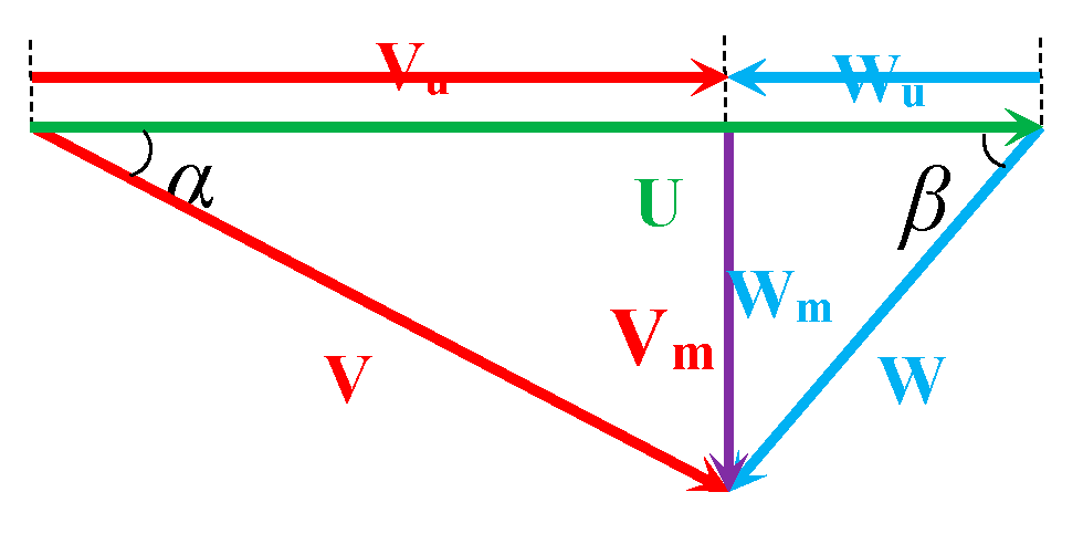
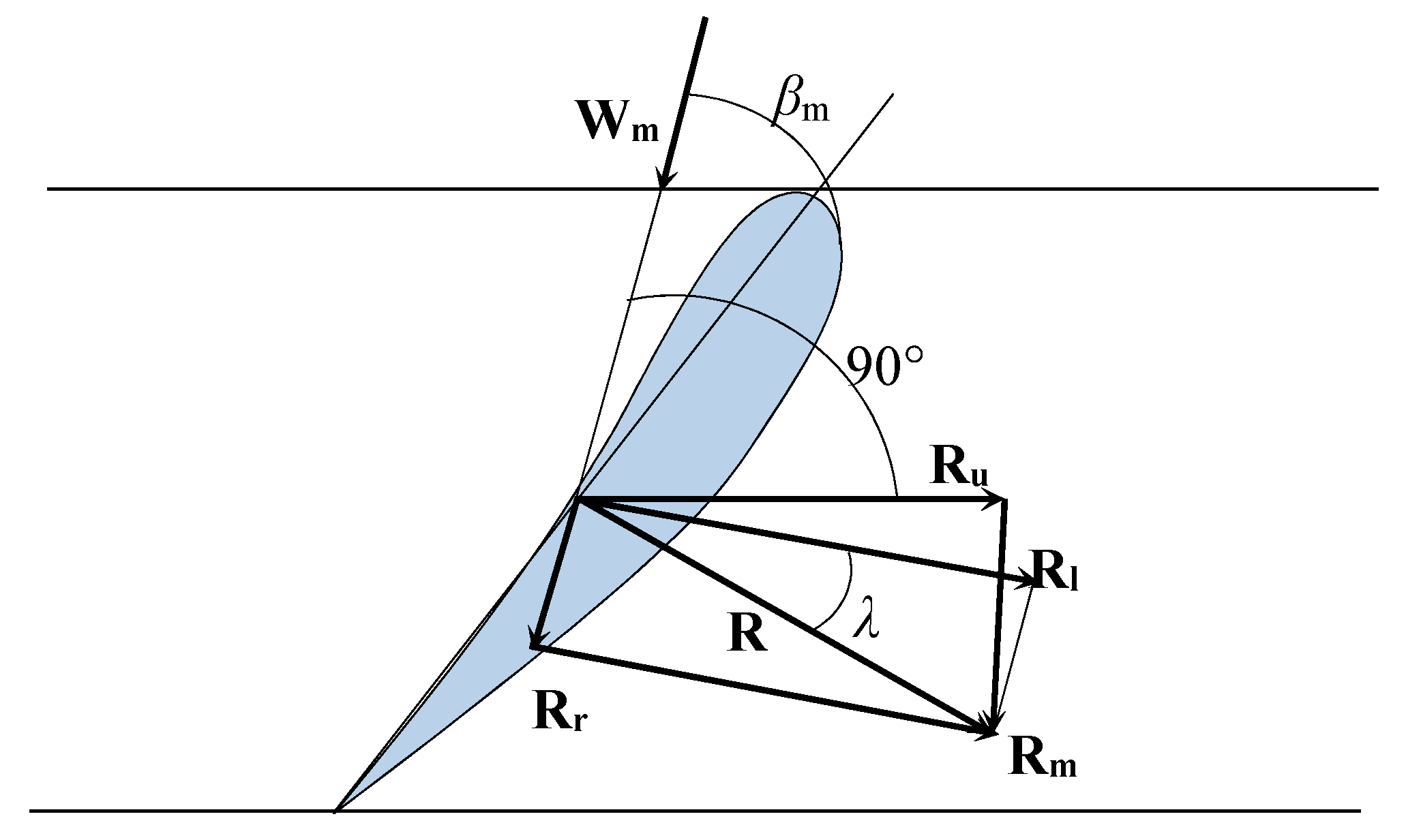
2.1.1. Hydraulic Forces on a Single Blade

Hydraulic instability is a complex, untraceable, and typical factor threatening the security and stability of hydropower stations, which is caused by the flow unbalance in the penstock, the spiral case, the guide vane and the hydro-turbine runner. According to many engineering observations [6,19], the hydraulic instability is mainly induced by the flow unbalance in the hydro-turbine runner, which can lead to the strong vibration of the HGSS. However, the research about the hydraulic instability in the hydro-turbine runner is poor. Therefore, we are going to establish a reasonable model to explain the hydraulic instability in the hydro-turbine runner.

To understand the hydraulic instability in the hydro-turbine runner, the stress characteristics for every hydro-turbine runner blade are firstly analyzed.

For the convenience of modeling, the flowing velocity of the water in the runner is decomposed along the blade direction and the runner peripheral direction, which can be defined as the relative velocity and the convected velocity, respectively. Figure 1 shows the triangle relationship among the convected velocity, the relative velocity and the absolute velocity in the blade inlet and outlet, in which W, U and V are the relative velocity, the convected velocity and the absolute velocity, respectively, α is the angle between convected velocity and absolute velocity, β is the angle between relative velocity and convected velocity, and the subscript 1 and 2, respectively represent the inlet and outlet of the blade. Figure 2 is the breakdown drawing for the velocity triangle.

For a single blade, the stress characteristics are shown in Figure 3 [34]. Here, the bold front stands for vector. Based on the Kutta-Joukowski theorem, the drag force and lift force [34] can be respectively written as

$$R_r=C_x\frac{\gamma }{g}\frac{{\left|{\mathbf{W}}_{\mathbf{m}}\right|}^2}{2}F,$$

(1)

and

$$R_l=C_y\frac{\gamma }{g}\frac{{\left|{\mathbf{W}}_{\mathbf{m}}\right|}^2}{2}F,$$

(2)

where R_r is the drag force; R_l is the lift force; C_x is the drag coefficient of the runner blade; C_y is the lift coefficient of the runner blade; F is the maximum projected area of a blade in the cascade for the hydro-turbine; W_m is the vector average value of the relative velocity of front and back flow around the blade, namely W_m = (W₁ + W₂)/2, W₁ is the inlet relative velocity of the runner blade, and W₂ is the exit relative velocity of the runner blade; W_m, W₁ and W₂ are vectors and |W_m|, |W₁|, and |W₂| are scalars, which represent the values of W_m, W₁ and W₂; γ is the unit weight of the liquids around the runner blade.

From Figure 3, the resultant force of drag force R_x and lift force R_y can be got as

$$R=\frac{R_l}{\cos \lambda }=C_y\frac{\gamma }{g}\frac{{\left|{\mathbf{W}}_{\mathbf{m}}\right|}^2}{2}\frac{F}{\cos \lambda },$$

(3)

where λ = arctan(C_x/C_y).

Then, decomposing the force R along the radial direction, the radial force R_m can be written as

$$R_m=C_y\frac{\gamma }{g}\frac{{\left|{\mathbf{W}}_{\mathbf{m}}\right|}^2}{2}\frac{F}{\cos \lambda }\cos \left({\beta }_m-\lambda \right),$$

(4)

where β_m is the direction angle of the average relative velocity.

From Figure 1 and Figure 2, the values of |W₁| and |W₂|can be obtained as

$$\left|{\mathbf{W}}_{\mathbf{1}}\right|=\frac{V_{m1}}{\sin {\beta }_1}=\frac{Q/F_1}{\sin {\beta }_1}=\frac{Q}{s_1\pi D_1{b}_0\sin {\beta }_1},$$

(5)

$$\left|{\mathbf{W}}_{\mathbf{2}}\right|=\frac{V_{m2}}{\sin {\beta }_2}=\frac{Q/F_2}{\sin {\beta }_2}=\frac{Q}{s_2\pi {D_2}^2\sin {\beta }_2},$$

(6)

where Q is the flow; s₁ and s₂ are the entrance excretion coefficient and exit excretion coefficient, respectively, s₁ = 1 − ZS_u/(πD₁), s₂ = 1 − ZS_u/(πD₂); Z is the number of the runner blades; S_u is the runner blade thickness; D₁ and D₂ are the entrance diameter and exit diameter of the runner blade, respectively; β₁ is the blade entrance flow angle; β₂ is the blade exit flow angle; b₀ is the guide vane height.

With regard to the blade entrance flow angle (β₁), according to Figure 2, it can be calculated as follows:

$${\beta }_1=\arctan \left(\frac{V_{m1}}{U_1-V_{u1}}\right)=\arctan (\frac{\frac{Q}{s_1\pi D_1{b}_0}}{\frac{D_1\omega }{2}-\frac{Q}{s_1\pi D_1{b}_0\tan {\alpha }_1}})=\arctan \left(\frac{2Q\tan {\alpha }_1}{\pi {D_1}^2\omega s_1{b}_0\tan {\alpha }_1-2Q}\right),$$

(7)

where α₁ is the guide vane angle; ω is the angular velocity.

Here, setting x-axis in the peripheral direction and y-axis in its perpendicular direction, which can be seen from Figure 1, W₁, W₂ and W_m can be written as

$${\mathbf{W}}_{\mathbf{1}}=\left(\left|{\mathbf{W}}_{\mathbf{1}}\right|\cos {\beta }_1,\left|{\mathbf{W}}_{\mathbf{1}}\right|\sin {\beta }_1\right),$$

(8)

$${\mathbf{W}}_{\mathbf{2}}=\left(\left|{\mathbf{W}}_{\mathbf{2}}\right|\cos {\beta }_2,\left|{\mathbf{W}}_{\mathbf{2}}\right|\sin {\beta }_2\right),$$

(9)

and

$${\mathbf{W}}_{\mathbf{m}}=\frac{{\mathbf{W}}_{\mathbf{1}}+{\mathbf{W}}_{\mathbf{2}}}{2}=\left(\frac{\left|{\mathbf{W}}_{\mathbf{1}}\right|\cos {\beta }_1+\left|{\mathbf{W}}_{\mathbf{2}}\right|\cos {\beta }_2}{2},\frac{\left|{\mathbf{W}}_{\mathbf{1}}\right|\sin {\beta }_1+\left|{\mathbf{W}}_{\mathbf{2}}\right|\sin {\beta }_2}{2}\right),$$

(10)

where |W_m| and β_m can be expressed as

$$\begin{array}{cc}\hfill \left|{\mathbf{W}}_{\mathbf{m}}\right|& =\frac{\sqrt{{(\left|{\mathbf{W}}_{\mathbf{1}}\right|\cos {\beta }_1+\left|{\mathbf{W}}_{\mathbf{2}}\right|\cos {\beta }_2)}^2+{(\left|{\mathbf{W}}_{\mathbf{1}}\right|\sin {\beta }_1+\left|{\mathbf{W}}_{\mathbf{2}}\right|\sin {\beta }_2)}^2}}{2}\hfill \\ & =\frac{Q}{2}\sqrt{\frac{1}{{(s_1\pi D_1{b}_0\sin {\beta }_1)}^2}+\frac{1}{{(s_2\pi {D_2}^2\sin {\beta }_2)}^2}+\frac{2\cos ({\beta }_2-{\beta }_1)}{s_1{s}_2{\pi }^2{D}_1{D_2}^2{b}_0\sin {\beta }_1\sin {\beta }_2}}\hfill \end{array},$$

(11)

and

$${\beta }_m=\arcsin \left(\frac{\left|{\mathbf{W}}_{\mathbf{1}}\right|\sin {\beta }_1+\left|{\mathbf{W}}_{\mathbf{2}}\right|\sin {\beta }_2}{\left|{\mathbf{W}}_{\mathbf{m}}\right|}\right)=\arcsin \left[\frac{2(s_1{D}_1{b}_0+s_2{D_2}^2)}{\sqrt{{\left(\frac{s_2{D_2}^2}{\sin {\beta }_1}\right)}^2+{\left(\frac{s_1{D}_1{b}_0}{\sin {\beta }_2}\right)}^2+\frac{2s_1{s}_2{D}_1{D_2}^2{b}_0\cos ({\beta }_2-{\beta }_1)}{\sin {\beta }_1\sin {\beta }_2}}}\right],$$

(12)

When the Reynolds number changes in the range from 10⁴ to 10⁶ and the range of attack angle is from 0.53 rad to 2.76 rad, the expressions of the lift coefficient and drag coefficient for the two-dimensional plate airfoil can be applied to hydro-turbine runner blade [35]. Therefore, one gets

$$\{\begin{array}{l}{C}_x=2{(\sin \upsilon )}^2\\ C_y=\sin 2\upsilon \end{array},$$

(13)

where υ is the attack angle.

According to Equation (13), one gets

$$\lambda =\arctan \left(\frac{C_x}{C_y}\right)=\arctan \left[\frac{2\sin {\left[\left(\arcsin C_y\right)/2\right]}^2}{C_y}\right],$$

(14)

Based on Equations (7), (11) and (14), Equation (4) can be written as

$$R_m=C_y\frac{Q^2}{8}\frac{\gamma }{g}\frac{F\cos \left({\beta }_m-\arctan \left[2\sin {\left(\left(\arcsin C_y\right)/2\right)}^2/C_y\right]\right)}{\cos \left\{\arctan \left[2\sin {\left(\left(\arcsin C_y\right)/2\right)}^2/C_y\right]\right\}}\times \left\{\begin{array}{l}\frac{1}{(s_1\pi D_1{b}_0\sin (\arctan (\frac{2Q\tan {\alpha }_1}{\pi {D_1}^2\omega s_1{b}_0\tan {\alpha }_1-2Q})){)}^2}+\frac{1}{{(s_2\pi {D_2}^2\sin {\beta }_2)}^2}\\ +\frac{2\cos ({\beta }_2-{\beta }_1)}{s_1{s}_2{\pi }^2{D}_1{D_2}^2{b}_0\sin (\arctan (\frac{2Q\tan {\alpha }_1}{\pi {D_1}^2\omega s_1{b}_0\tan {\alpha }_1-2Q}))\sin {\beta }_2}\end{array}\right\},$$

(15)

where

$${\beta }_m=\arcsin \left[2\left(s_1{D}_1{b}_0+s_2{D_2}^2\right)/\sqrt{{\left(\frac{s_2{D_2}^2}{\sin {\beta }_1}\right)}^2+{\left(\frac{s_1{D}_1{b}_0}{{D_2}^2\sin {\beta }_2}\right)}^2+\frac{2s_1{s}_2{D}_1{D_2}^2{b}_0\cos ({\beta }_2-{\beta }_1)}{\sin {\beta }_1\sin {\beta }_2}}\right].$$

(16)

Defining ξ as the position angle of the blade, R_m can be broken down to the component in x and y directions of Cartesian coordinate system, which can be written as

$$\{\begin{array}{l}{R}_x=R_m\cos \xi \\ R_y=R_m\sin \xi \end{array},$$

(17)

where ξ = ξ₀ + ωt, ξ₀ is the initial position angle of a selected blade.

2.1.2. Hydraulic Forces on a Single Blade

In the ideal condition, all blades of the runner have the same exit flow angle β₂, and the total radial hydraulic force of all runner blades is zero. However, in actual engineering, for the hydro-turbine blades, due to the manufacturing error, the deformation and the wear in the operation, there are always differences in the exit flow angles, which cause that the total radial hydraulic force is not zero. Further, the radial unbalance hydraulic force in the hydro-turbine runner can lead to the strong vibration of the HGSS. Here, for simplifying the calculation, we are going to make two assumptions.

Assumption 1.

The number of blades for the hydro-turbine runner is even.

Assumption 2.

Only one blade’s exit flow angle is inconsistent with the other blades, and the deviation of the exit flow angle is χ.

Based on Assumptions 1 and 2, and combining Equations (15) and (17), the hydraulic unbalance force acting on the hydro-turbine runner in x and y directions of Cartesian coordinate system can be written as

$$\begin{array}{l}{P}_x=\left|\cos \alpha \right|C_y\frac{Q^2}{8}\frac{\gamma }{g}\frac{F}{\cos \left\{\arctan \left[2\sin {\left(\left(\arcsin C_y\right)/2\right)}^2/C_y\right]\right\}}\\ \times \left\{\begin{array}{c}\cos \left({\beta }_{m1}-\arctan (\frac{2\sin (\frac{\arcsin C_y}{2}{)}^2}{Cy})\right)\times \left\{\begin{array}{l}\frac{1}{(s_1\pi D_1{b}_0\sin (\arctan (\frac{2Q\tan {\alpha }_1}{\pi {D_1}^2\omega s_1{b}_0\tan {\alpha }_1-2Q})){)}^2}+\frac{1}{(s_2\pi {D_2}^2\sin {\beta }_{21}{)}^2}\\ +\frac{2\cos ({\beta }_{21}-{\beta }_1)}{s_1{s}_2{\pi }^2{D}_1{D_2}^2{b}_0\sin (\arctan (\frac{2Q\tan {\alpha }_1}{\pi {D_1}^2\omega s_1{b}_0\tan {\alpha }_1-2Q}))\sin {\beta }_{21}}\end{array}\right\}-\\ \cos \left({\beta }_{m2}-\arctan (\frac{2\sin (\frac{\arcsin C_y}{2}{)}^2}{C^y})\right)\times \left\{\begin{array}{l}\frac{1}{(s_1\pi D_1{b}_0\sin (\arctan (\frac{2Q\tan {\alpha }_1}{\pi {D_1}^2\omega s_1{b}_0\tan {\alpha }_1-2Q})){)}^2}+\frac{1}{(s_2\pi {D_2}^2\sin {\beta }_{22}{)}^2}\\ +\frac{2\cos ({\beta }_{22}-{\beta }_1)}{s_1{s}_2{\pi }^2{D}_1{D_2}^2{b}_0\sin (\arctan (\frac{2Q\tan {\alpha }_1}{\pi {D_1}^2\omega s_1{b}_0\tan {\alpha }_1-2Q}))\sin {\beta }_{22}}\end{array}\right\}\end{array}\right\}\end{array},$$

(18)

and

$$\begin{array}{cc}\hfill P_y& =\left|\sin \alpha \right|C_y\frac{Q^2}{8}\frac{\gamma }{g}\frac{F}{\cos \left\{\arctan \left[2\sin {\left(\left(\arcsin C_y\right)/2\right)}^2/C_y\right]\right\}}\hfill \\ \\ & \times \left\{\begin{array}{c}\cos \left({\beta }_{m1}-\arctan (\frac{2\sin (\frac{\arcsin C_y}{2}{)}^2}{C_y})\right)\times \left\{\begin{array}{l}\frac{1}{(s_1\pi D_1{b}_0\sin (\arctan (\frac{2Q\tan {\alpha }_1}{\pi {D_1}^2\omega s_1{b}_0\tan {\alpha }_1-2Q})){)}^2}+\frac{1}{(s_2\pi {D_2}^2\sin {\beta }_{21}{)}^2}\\ +\frac{2\cos ({\beta }_{21}-{\beta }_1)}{s_1{s}_2{\pi }^2{D}_1{D_2}^2{b}_0\sin (\arctan (\frac{2Q\tan {\alpha }_1}{\pi {D_1}^2\omega s_1{b}_0\tan {\alpha }_1-2Q}))\sin {\beta }_{21}}\end{array}\right\}-\\ \cos \left({\beta }_{m2}-\arctan (\frac{2\sin (\frac{\arcsin C_y}{2}{)}^2}{C_y})\right)\times \left\{\begin{array}{l}\frac{1}{(s_1\pi D_1{b}_0\sin (\arctan (\frac{2Q\tan {\alpha }_1}{\pi {D_1}^2\omega s_1{b}_0\tan {\alpha }_1-2Q})){)}^2}+\frac{1}{(s_2\pi {D_2}^2\sin {\beta }_{22}{)}^2}\\ +\frac{2\cos ({\beta }_{22}-{\beta }_1)}{s_1{s}_2{\pi }^2{D}_1{D_2}^2{b}_0\sin (\arctan (\frac{2Q\tan {\alpha }_1}{\pi {D_1}^2\omega s_1{b}_0\tan {\alpha }_1-2Q}))\sin {\beta }_{22}}\end{array}\right\}\end{array}\right\}\hfill \end{array},$$

(19)

where β₂₁ and β₂₂ are the blade exit flow angle of the pair of symmetrical blades; β_m1 and β_m2 are the direction angle of the average relative velocity of the pair of symmetrical blades, and

$${\beta }_{m1}=\arcsin \left[2\left(s_1\pi D_1{b}_0+s_2\pi {D_2}^2\right)/\sqrt{{\left(\frac{s_2\pi {D_2}^2}{\sin {\beta }_1}\right)}^2+{\left(\frac{s_1\pi D_1{b}_0}{{D_2}^2\sin {\beta }_{21}}\right)}^2+\frac{2s_1{s}_2{\pi }^2{D}_1{D_2}^2{b}_0}{\sin {\beta }_1\sin {\beta }_{21}}}\right],$$

(20)

$${\beta }_{m2}=\arcsin \left[2\left(s_1\pi D_1{b}_0+s_2\pi {D_2}^2\right)/\sqrt{{\left(\frac{s_2\pi {D_2}^2}{\sin {\beta }_1}\right)}^2+{\left(\frac{s_1\pi D_1{b}_0}{{D_2}^2\sin {\beta }_{22}}\right)}^2+\frac{2s_1{s}_2{\pi }^2{D}_1{D_2}^2{b}_0}{\sin {\beta }_1\sin {\beta }_{22}}}\right],$$

(21)

2.2. Modeling of the Mechanical and Electrical Unbalance Forces

2.2.1. Damping Force Model

When the hydro-turbine generator unit is in a steady state, the damping forces [31] on the shaft system can be expressed as

$$\{\begin{array}{l}{F}_{x-f}=c{\dot{x}}_{o1}\\ F_{y-f}=c{\dot{y}}_{o1}\end{array},$$

(22)

where c is damped coefficient; (x_o1 and y_o1) are axis coordinates of the hydro-turbine generator rotor.

2.2.2. Oil Film Force Model

When the hydro-turbine generator unit is in a stable operation with a small perturbation, and the unsteady boundary of the oil film is set to be a steady boundary, the oil film force [31] is adopted as

$$\{\begin{array}{l}{F}_{x-oil}=F_{x0}+k_{xx}{x}_{o1}+k_{xy}{y}_{o1}+d_{xx}{\dot{x}}_{o1}+d_{xy}{\dot{y}}_{o1}\\ F_{y-oil}=F_{y0}+k_{yx}{x}_{o1}+k_{yy}{y}_{o1}+d_{yx}{\dot{x}}_{o1}+d_{yy}{\dot{y}}_{o1}\end{array},$$

(23)

where F_x0 and F_y0 are oil film forces in the quiescent operation point; k_xx, k_xy, k_yx, k_yy, d_xx, d_xy, d_yx and d_yy are coefficients, which can be obtained from reference [31].

2.2.3. Rub-Impact Force Model

In the case of misalignment failure of hydro-turbine generator set, there is a great possibility of friction between the rotor and stator. In this paper, the rubbing force model assumes that there is an elastic collision between the rotor and stator, and the rubbing force is determined by the rotor, stator and the stiffness of spindle, and the thermal effect produced by the rubbing action is ignored. Thus, the rub-impact force model [19] can be written as

$$\left\{\begin{array}{l}{F}_{x-rub}\\ F_{y-rub}\end{array}\right\}=-H(L-\delta )\frac{(L-\delta )k_c}{L}\left[\begin{array}{ll}1& -f\\ f& 1\end{array}\right]\left\{\begin{array}{l}{x}_{o1}\\ y_{o1}\end{array}\right\},$$

(24)

where f is the relevant friction coefficient; k_c is the stator stiffness; δ is the gap between the generator rotor and stator; L is the radical displacement of the generator rotor axis (o₁);

$$H(x_{o1})=\{\begin{array}{ll}0& x_{o1}\le 0\\ 1& x_{o1}>0\end{array}.$$

(25)

2.2.4. Unbalanced Magnetic Pull Model

When the number of the pole pairs of a hydro-turbine generator is more than three, the unbalanced magnetic pull of the hydro-turbine generator [19] can be described as

$$\{\begin{array}{l}{F}_{x-ump}=\frac{r_{1}l\pi k_j^2{i}^2}{4{\mu }_{0}L}\left(2{\mathsf{\Lambda }}_0{\mathsf{\Lambda }}_1+{\mathsf{\Lambda }}_1{\mathsf{\Lambda }}_2+{\mathsf{\Lambda }}_2{\mathsf{\Lambda }}_3\right)x_{o1}\\ F_{y-ump}=\frac{r_{1}l\pi k_j^2{i}^2}{4{\mu }_{0}L}\left(2{\mathsf{\Lambda }}_0{\mathsf{\Lambda }}_1+{\mathsf{\Lambda }}_1{\mathsf{\Lambda }}_2+{\mathsf{\Lambda }}_2{\mathsf{\Lambda }}_3\right)y_{o1}\end{array},$$

(26)

where r₁ is the rotor radius; μ₀ is the air permeability; k_j is the air gap flux potential; i is the generator excitation current; l is the generator rotor length. Apart from the above, there are four meaningless intermediate variables (Λ₀, Λ₁, Λ₂, and Λ₃) calculated in reference [14].

2.3. Modeling of the HGSS

The hydro-turbine generator shafting is installed in a vertical position. In this paper, we only consider the transverse vibration, neglecting the forces of the thrust bearing.

Assumption 3.

The rotor and the coupling are both rigid.

The coordinate relationships [36] of generator rotor (o₁), and the hydro-turbine runner (o₂) are shown in Figure 4.

From Figure 4, one gets

$$\{\begin{array}{l}{x}_{o2}=x_{o1}+r\cos \theta \\ y_{o2}=y_{o1}+r\sin \theta \\ x_{c1}=x_{o1}+e_1\cos \phi \\ y_{c1}=y_{o1}+e_1\sin \phi \\ x_{c2}=x_{o2}+e_2\cos \phi \\ y_{c2}=y_{o2}+e_2\sin \phi \end{array},$$

(27)

where (x_o2, y_o2) represent the axis coordinates of the hydro-turbine runner; θ₀ is the initial angle for the hydro-turbine generator unit, and θ = ωt + θ₀; φ₀ represents the initial angle of the generator rotor, and φ = ωt + φ₀; r is the distance between o₁ and o₂; (x_c1, y_c1) and (x_c2, y_c2) are the mass center coordinates of the generator rotor and the hydro-turbine runner, severally; e₁ and e₂ are the mass eccentricity of the generator rotor and hydro-turbine runner, respectively.

The potential energy and kinetic energy of the HGSS can be expressed as

$$\{\begin{array}{cc}\hfill T& =T_r+T_G=\frac{1}{2}(J_1+m_1{e}_1^2){\dot{\phi }}^2+\frac{1}{2}\left[J_1+m_2\left(r^2+e_2^2\right)\right]{\dot{\theta }}^2\hfill \\ & +\frac{1}{2}{m}_1({\dot{x}}_{o1}^2+{\dot{y}}_{o1}^2+e_1^2{\dot{\phi }}^2-2{\dot{x}}_{o1}{e}_1\dot{\phi }\sin \phi +2{\dot{y}}_{o1}{e}_1\dot{\phi }\cos \phi )\hfill \\ & +\frac{1}{2}{m}_2({\dot{x}}_{o2}^2+{\dot{y}}_{o2}^2+e_2^2{\dot{\phi }}^2-2{\dot{x}}_{o2}{e}_2\dot{\phi }\sin \phi +2{\dot{y}}_{o2}{e}_2\dot{\phi }\cos \phi )\hfill \\ \hfill U& =\frac{1}{2}{k}_1{\left|o{o}_1\right|}^2+\frac{1}{2}{k}_2{\left|o{o}_2\right|}^2=\frac{1}{2}{k}_1\left(x_{o1}^2+y_{o1}^2\right)\hfill \\ & +\frac{1}{2}{k}_2\left(x_{o1}^2+y_{o1}^2+2r{x}_{o1}\cos \theta +2r{y}_{o1}\sin \theta +r^2\right)\hfill \end{array},$$

(28)

where J₁ is the moment of inertia of the generator; J₂ is the moment of inertia of the turbine; m₁ is the mass of the rotor; T is the total kinetic energy; U is the total potential energy; k₁ is the bearing stiffness of the generator rotor; k₂ is the bearing stiffness of the hydro-turbine runner.

The Lagrange function of the HGSS is defined as the difference between kinetic energy and potential energy, which can be written as

$$\begin{array}{cc}\hfill L& =T-U\hfill \\ & =\frac{1}{2}\left(J_1+m_1{e}_1^2\right){\dot{\phi }}^2+\frac{1}{2}\left[J_1+m_2\left(r^2+e_2^2\right)\right]{\dot{\theta }}^2-\frac{1}{2}{k}_2\left(x_{o1}^2+y_{o1}^2+2r{x}_{o1}\cos \theta +2r{y}_{o1}\sin \theta +r^2\right)\hfill \\ & +\frac{1}{2}{m}_2\left({{\dot{x}}_{o2}}^2+{{\dot{y}}_{o2}}^2+e_2^2{\dot{\phi }}^2-2{\dot{x}}_{o2}{e}_2\dot{\phi }\sin \phi +2{\dot{y}}_{o2}{e}_2\dot{\phi }\cos \phi \right)-\frac{1}{2}{k}_1\left(x_{o1}^2+y_{o1}^2\right)\hfill \\ & +\frac{1}{2}{m}_1\left({{\dot{x}}_{o1}}^2+{{\dot{y}}_{o1}}^2+e_1^2{\dot{\phi }}^2-2{\dot{x}}_{o1}{e}_1\dot{\phi }\sin \phi +2{\dot{y}}_{o1}{e}_1\dot{\phi }\cos \phi \right)\hfill \end{array}.$$

(29)

The Lagrange equations [37] of the HGSS is

$$\{\begin{array}{l}\frac{d}{dt}\left(\frac{\partial L}{\partial {\dot{x}}_{o1}}\right)-\frac{\partial L}{\partial x_{o1}}=\mathsf{\Sigma }{F}_x\\ \frac{d}{dt}\left(\frac{\partial L}{\partial {\dot{y}}_{o1}}\right)-\frac{\partial L}{\partial y_{o1}}=\mathsf{\Sigma }{F}_y\end{array}.$$

(30)

Then, the dynamic model of the HGSS can be described as

$$\{\begin{array}{cc}\hfill \frac{d}{dt}\left(\frac{\partial L}{\partial {\dot{x}}_{o1}}\right)-\frac{\partial L}{\partial x_{o1}}& =\left(m_1+m_2\right){\ddot{x}}_{o1}-\left[\left(m_1{e}_1+m_2{e}_2\right)\sin \phi +m_{2}r\sin \theta \right]\hfill \\ & -\left[\left(m_1{e}_1+m_2{e}_2\right)\cos \phi +m_{2}r\cos \theta \right]{\omega }^2-\left(k_1+k_2\right)x_{o1}+k_{2}r\cos \theta \hfill \\ & =F_{x-ump}+F_{x-oil}-F_{x-f}+P_x+F_{x-rub}\hfill \\ \hfill \frac{d}{dt}\left(\frac{\partial L}{\partial {\dot{y}}_{o1}}\right)-\frac{\partial L}{\partial y_{o1}}& =\left(m_1+m_2\right){\ddot{y}}_{o1}+\left[\left(m_1{e}_1+m_2{e}_2\right)\cos \phi +m_{2}r\cos \theta \right]\hfill \\ & -\left[\left(m_1{e}_1+m_2{e}_2\right)\sin \phi +m_{2}r\sin \theta \right]{\omega }^2+\left(k_1+k_2\right)y_{o1}+k_{2}r\sin \theta \hfill \\ & =F_{y-ump}+F_{y-oil}-F_{y-f}+P_y+F_{y-rub}\hfill \end{array}.$$

(31)

Furthermore, Equation (31) can be simplified as

$$\{\begin{array}{l}{\dot{x}}_{o1}=v_x\\ {\dot{v}}_x=\left\{\begin{array}{l}\left[\left(m_1{e}_1+m_2{e}_2\right)\cos \phi +m_{2}r\cos \theta \right]{\omega }^2+\left(k_1+k_2\right)x_{o1}-k_{2}r\cos \theta \\ +F_{x-ump}+F_{x-oil}-F_{x-f}+P_x+F_{x-rub}\end{array}\right\}/\left(m_1+m_2\right)\\ {\dot{y}}_{o1}=v_y\\ {\dot{v}}_y=\left\{\begin{array}{l}\left[\left(m_1{e}_1+m_2{e}_2\right)\sin \phi +m_{2}r\sin \theta \right]{\omega }^2-\left(k_1+k_2\right)y_{o1}-k_{2}r\sin \theta \\ +F_{y-ump}+F_{y-oil}-F_{y-f}+P_y+F_{y-rub}\end{array}\right\}/\left(m_1+m_2\right)\end{array}.$$

(32)

3. Dynamic Simulation and Analyses

In this section, by applying the Runge–Kutta method to the numerical simulation, the effects of the deviation of the blade exit flow angle (χ), the blade exit diameter (D₂), the guide vane opening angle (α₁) on the nonlinear dynamic characteristics of the HGSS are analyzed. The step–size is 0.01, the iteration steps are 5000 for each time of simulation, and the initial values [36] specified for the computation are as follows: [x_o1, v_x, y_o1, v_y] = [0.0001, 0.0001, 0.0001, 0.0001]. Besides, based on references [36,38], the values of the parameters involved in the computation are chosen as follows: m₁ = 1.5 × 104 kg, m₂ = 1.1 × 104 kg, c = 6.5 × 104 N·s/m, k₁ = 8.5 × 107 N/m, k₂ = 6.5 × 107 N/m, e₁ = 0.0005 m, e₂ = 0.0005 m, i = 800 A, m₃ = 1.0 × 103 kg, ω = 3.925 rad/s, Δd = 0.0001068 m, l = 5.0 m, Δl = 0.0002 m, μ₀ = 4π × 10⁻⁷ H/m, δ = 0.008 m, f = 0.012, K_c = 3 × 107 N/m, Q = 42.86 m³/s, C_y = 0.5, D₁ = 2.0 m, b₀ = 0.5 m, Φ = 0 rad, θ₀ = 1 rad, φ₀ = 0.8 rad.

3.1. Model Verification

To study the influences of the hydraulic instability on the vibration performance of the HTGS, and verify the rationality of the model presented in Section 2, a comparison between the model in this paper and the one in reference [36] is presented. In reference [36], the hydraulic instability factor was not considered. As is shown in Figure 5, the vibration amplitude of the axis coordinates (x_o1 and y_o1) in the model of this paper is far larger than that in the previous model in reference [36], meaning that the hydraulic instability can aggravate the vibration of the HGSS. In fact, the influences of the hydraulic instability have been detected in the actual hydropower stations, and a typical feature is to magnify the vibration amplitude of the HGSS. Based on these analyses, it can be discovered that the model presented in this paper is more reasonable than the one which doesn’t consider the hydraulic unbalance force. Then, some more detailed analyses are carried out in Section 3.2, Section 3.3 and Section 3.4.

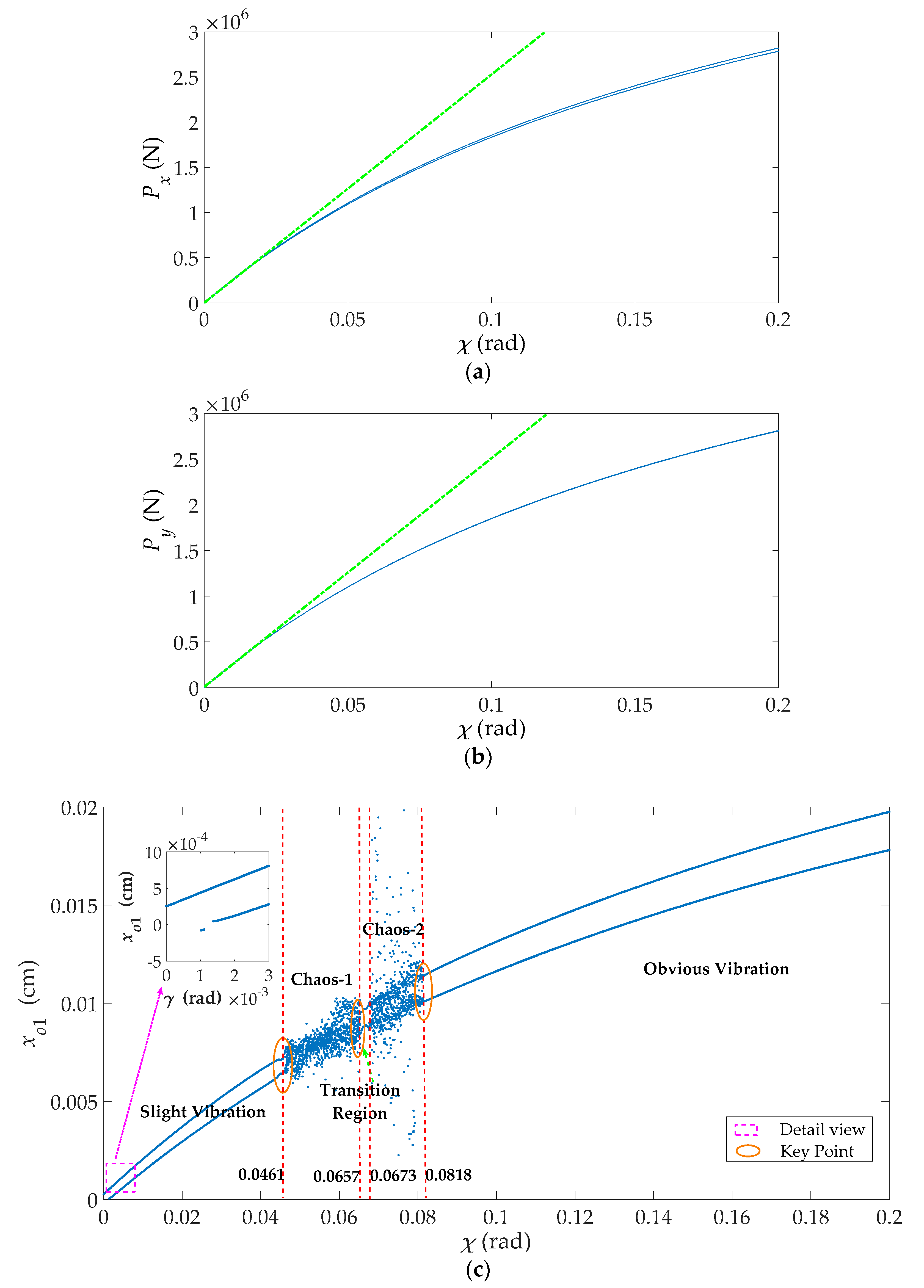
3.2. Effects of the Deviation of the Blade Exit Flow Angle (χ)

The deviation of the blade exit flow angle (χ) is one of the most crucial factors causing the hydraulic instability. In order to study the dynamic characteristics of the hydro-turbine generator unit with the deviation of the blade exit flow angle (χ), the bifurcation diagrams of the hydraulic unbalance forces (P_x and P_y) and the generator rotor axis coordinates (x_o1 and y_o1) with the increasing deviation of the blade exit flow angle (χ) are shown in Figure 6.

As is shown in Figure 6a,b, with the increase of the derivation of the blade exit flow angle (χ) from 0 rad to 0.2 rad, the hydraulic unbalance forces (P_x and P_y) increase with a decreasing growth rate. At the same time, under the effects of the hydraulic unbalance forces (P_x and P_y), the vibration amplitude of the axis coordinates (x_o1 and y_o1) increases gradually when 0 rad < χ < 0.2 rad, which can be seen in Figure 6c,d.

In addition, taking a further study of Figure 6c,d, more dynamic characteristics of the axis coordinates (x_o1 and y_o1) can be obtained. In detail, in the range of 0 rad < χ < 0.0461 rad, the axis coordinates (x_o1 and y_o1) keep in a slight vibration, and the vibration amplitude gradually increases. Specially, a small fluctuation appears at the end of this range, which finally induces the chaos named Chaos-1 at χ = 0.0461 rad. Then the axis coordinates (x_o1 and y_o1) get rid of the chaos and entered into a transient period-2 oscillation when 0.0657 rad < χ < 0.0673 rad. Interestingly, at χ = 0.0673 rad, the axis coordinates (x_o1 and y_o1) turn into a new chaos state named Chaos-2. Finally, when 0.0818 rad < χ < 0.2 rad, the axis coordinates (x_o1 and y_o1), once again, enter into a period-2 oscillation.

In light of the above analyses, there are several points that needed to be focused on. First, a small increase of the derivation of the blade exit flow angle (χ) could cause an apparent increase of the hydraulic unbalance forces (P_x and P_y), which can further cause a large vibration of the shafting. Second, according to the similar changing trend of the hydraulic unbalance forces (P_x and P_y) and axis coordinates (x_o1 and y_o1), it can be found that the hydraulic instability determines the overall changing trend of the shafting behaviors. Third, in the ranges of the 0.0461 rad < χ < 0.0657 rad and 0.0673 rad < χ < 0.0818 rad, the axis coordinates (x_o1 and y_o1) are in a chaos state while the hydraulic unbalance forces show period oscillation, which is because that the hydraulic instability can cause the mechanical and electrical instability. In other words, the chain reaction among the hydraulic, mechanical and electrical instability happens in these ranges. Third, when 0.0818 rad < χ < 0.2 rad, although the axis coordinates (x_o1 and y_o1) get rid of the chaos, the vibration amplitude of the shafting is very large, which can cause the mechanical fatigue and even destroy the hydro-turbine. Therefore, in actual engineering, the derivation of the blade exit flow angle (χ) should be limited in the range from 0 rad to 0.0461 rad.

3.3. Effects of the Blade Exit Diameter (D₂)

In addition to the deviation of the blade exit flow angle (χ), the size of the runner can also influence the hydraulic characteristics of the hydro-turbine. Here, to investigate the effects of the size of the runner, the bifurcation diagrams of the hydraulic unbalance forces (P_x and P_y) and the axis coordinates (x_o1 and y_o1) with the increasing blade exit diameter (D₂) are presented in Figure 7.

From Figure 7a,b, it can be seen that dynamic characteristics of the hydraulic unbalance forces (P_x and P_y) with the increasing blade exit diameter (D₂) are more complex than that of the deviation of the blade exit flow angle (χ). Concretely, when 0.37 m < D₂ < 0.4824 m, the hydraulic unbalance forces (P_x and P_y) decrease rapidly. However, at the point of D₂ = 0.4824 m, the changing trend of the hydraulic unbalance forces (P_x and P_y) shows a dramatical turn. Then, the hydraulic unbalanced forces (P_x and P_y) keep in a quick increase when 0.5522 m < D₂ < 0.6372 m and maintain stability when 0.5522 m < D₂ < 0.6372 m. Particularly, at the point of D₂ = 0.6372 m, a HOPF bifurcation appears, which is a dynamic bifurcation meaning that with the system parameter changing continuously to the bifurcation point, the stability of the system changes suddenly. Finally, in the range of 0.8046 m < D₂ < 1.6 m, the hydraulic unbalance forces (P_x and P_y) remain in a slow growth.

Comparing the bifurcation diagrams of the hydraulic unbalanced forces (P_x and P_y) and the axis coordinates (x_o1 and y_o1), it can be found that when 0.4 m < D₂ < 0.8 m, the overall changing trend of them are similar, but the dynamic characteristics of the axis coordinates (x_o1 and y_o1) are more complex. Specifically speaking, the axis coordinates (x_o1 and y_o1) present Chaos-1, Chaos-2 and Chaos-3 in the ranges of 0.4664 m < D₂ < 0.4701 m, 0.4706 m < D₂ < 0.4767 m, and 0.5255 m < D₂ < 0.7065 m, respectively. Then, when D₂ > 0.8 m, the hydraulic unbalance forces (P_x and P_y) increase with the changing of the runner blade exit diameter, on the contrary, the vibration amplitude of the axis coordinates (x_o1 and y_o1) gradually decreases. Meanwhile, at the point of D₂ = 0.9505 m and D₂ = 1.041 m, the axis coordinates (x_o1 and y_o1) respectively enter into Chaos-4 and Chaos-5.

Based on above analyses, some important results can be got. First, for different blade exit diameters (D₂), the value of the hydraulic unbalance forces has visible differences. Second, according to the differences in the changing trend of the hydraulic unbalanced forces (P_x and P_y) and axis coordinates (x_o1 and y_o1), it can be found that when the blade exit diameter (D₂) is small, the hydraulic unbalance forces (P_x and P_y) can determine the overall changing trend of the vibration amplitude of the axis coordinates (x_o1 and y_o1). However, when the blade exit diameter (D₂) is large, it can weaken the influence of the hydraulic unbalance forces (P_x and P_y) caused by the blade manufacturing error. Besides this, in the ranges of 0.4664 m < D₂ < 0.4701 m, 0.4706 m < D₂ < 0.4767 m, and 0.5255 m < D₂ < 0.7065 m, the hydraulic unbalance forces (P_x and P_y) are in period oscillation while the axis coordinates (x_o1 and y_o1) are in chaos, which indicates that the hydraulic instability can induce the mechanical and electrical instability, and the chain reaction among them can cause the chaos of axis coordinates (x_o1 and y_o1). Finally, in the range from 0.7065 m to 0.9505 m, the axis coordinates (x_o1 and y_o1) show an abnormal change due to the HOPF bifurcation. Therefore, the best range of the blade exit diameter is from 1.215 m to 1.6 m.

3.4. Effects of the Guide Vane Opening Angle (α₁)

In previous sections, the dynamic characteristics of the HGSS with the changing deviation of the blade exit flow angle (χ) and blade exit diameter (D₂) have been studied. These two factors are mainly related to the design and manufacture of the hydro-turbine runner. In fact, in the actual hydropower station, the operation condition is also a critical factor influencing the stability of the HGSS. In the starting, shutdown and load changing process, the guide vane all needs to be adjusted to adapt the current operation condition. Therefore, the effects of the guide vane opening angle on the HGSS are needed to be studied. And bifurcation diagrams of the hydraulic unbalanced forces (P_x and P_y) and the axis coordinates (x_o1 and y_o1) with the guide vane opening angle (α₁) increasing from 0 rad to 0.8 rad are shown in Figure 8.

From Figure 8a,b, when 0 rad < α₁ < 0.1331 rad, the hydraulic unbalance forces (P_x and P_y) are very large, and they decrease rapidly with the guide vane opening angle (α₁) increasing. Then, at the point of α₁ = 0.1331 rad, the HOPF bifurcation appears. Finally, when α₁ > 0.1713 rad, the hydraulic unbalance forces (P_x and P_y) maintain a stable periodic oscillation.

As is shown in Figure 8c,d, the overall changing trend of the axis coordinates (x_o1 and y_o1) is similar with the hydraulic unbalance forces (P_x and P_y). However, some differences between the axis coordinates (x_o1 and y_o1) and the hydraulic unbalance forces (P_x and P_y) needed to be concerned about in the details. Concretely, when 0.0154 rad < α₁ < 0.0173 rad and 0.0181 rad < α₁ < 0.0235 rad, the hydraulic unbalance forces (P_x and P_y) keep in period oscillation while the axis coordinates (x_o1 and y_o1) keep in Chaos-1 and Chaos-2, respectively.

According to the above analyses, four important results can be obtained. First, the vibration amplitude of the axis coordinates (x_o1 and y_o1) is very large when the guide vane opening angle is small. Namely, when the hydro-turbine generator unit works in the low load condition, the shafting vibration is strong, which is consistent with the actual engineering observation. Second, the hydraulic unbalance forces (P_x and P_y) and the vibration amplitude of axis coordinates (x_o1 and y_o1), show a similar changing trend, meaning that the hydraulic instability can determine the overall changing trend of axis coordinates (x_o1 and y_o1). Third, based on the differences between the hydraulic unbalance forces (P_x and P_y) and the axis coordinates (x_o1 and y_o1) in the ranges of 0.0154 rad < α₁ < 0.0173 rad and 0.0181 rad < α₁ < 0.0235 rad, it can be determined that under the influences of the hydraulic instability, the electrical and mechanical instability are enhanced, which can lead to chaos in the shafting system. Finally, when 0.1331 rad < α₁ < 0.1713 rad, because of the HOPF bifurcation, the vibration amplitude of the axis coordinates (x_o1 and y_o1) abnormally changes, which needs to closely watched in the operation. Therefore, in actual engineering, the safe range of the guide vane opening angle is from 0.1713 rad to 0.8 rad.

4. Conclusions

In this paper, based on the Kutta-Joukowski theorem, a mathematical model of the hydraulic unbalance forces is established. Then, combining the mechanical and electrical unbalance factors, a novel nonlinear mathematical model of the HGSS is presented. Besides this, using the numerical computation method, the dynamic characteristics of the HGSS are studied with the changing of the deviation of the blade exit flow angle, the blade exit diameter and the guide vane opening angle. Fortunately, some meaningful results have been found.

(1) A small increase of the derivation of the blade exit flow angle (χ) could cause an apparent increase of the hydraulic unbalance forces and further magnify the vibration amplitude of the HTGS. Moreover, the hydraulic instability can determine the overall changing trend of the shafting dynamic behaviors.

(2) The larger blade exit diameter can weaken the effects of the hydraulic instability on the shafting system. The best range of the blade exit diameter is from 1.215 m to 1.6 m.

(3) The vibration amplitude of the axis coordinates (x_o1 and y_o1) in the small guide vane opening angle is larger than that in the large guide vane opening angle. At the same time, a safe range of the guide vane opening angle is from 0.1713 rad to 0.8 rad.

More importantly, these results can provide a theoretical reference for the further study of the hydraulic instability, the design and manufacturing of the hydro-turbine runner blade and the operation of the hydropower station.

References

1. Paish, O. Micro-hydropower: Status and prospects. Proc. Inst. Mech. Eng. Part A J. Power Energy 2005, 216, 31–40. [Google Scholar] [CrossRef]
2. Spänhoff, B. Current status and future prospects of hydropower in Saxony (Germany) compared to trends in Germany, the European Union and the World. Renew. Sustain. Energy Rev. 2014, 30, 518–525. [Google Scholar] [CrossRef]
3. Modesto, P.S.; Francisco, J.S.; Helena, M.R.; Amparo, L.J. Energy Recovery in Existing Water Networks: Towards Greater Sustainability. Water 2017, 2, 97. [Google Scholar] [CrossRef]
4. Xu, B.B.; Chen, D.Y.; Behrens, P.; Ye, W.; Guo, P.C.; Luo, X.Q. Modeling oscillation modal interaction in a hydroelectric generating system. Energy Convers. Manag. 2018, 174, 208–217. [Google Scholar] [CrossRef]
5. Chu, S.; Majumdar, A. Opportunities, and challenges for a sustainable energy future. Nature 2012, 488, 294–303. [Google Scholar] [CrossRef] [PubMed]
6. Giosio, D.R.; Henderson, A.D.; Walker, J.M.; Brandner, P.A. Rapid Reserve Generation from a Francis Turbine for System Frequency Control. Energies 2017, 10, 496. [Google Scholar] [CrossRef]
7. Zhang, L.K.; Ma, Z.Y.; Wu, Q.Q.; Wang, X.N. Vibration analysis of coupled bending-torsional rotor-bearing system for hydraulic generating set with rub-impact under electromagnetic excitation. Arch. Appl. Mech. 2016, 86, 1665–1679. [Google Scholar] [CrossRef]
8. Martinez-Lucas, G.; Sarasua, J.I.; Sanchez-Fernandez, J.A.; Wilhelmi, J.R. Frequency control support of a wind-solar isolated system by a hydropower plant with long tail-race tunnel. Renew. Energy 2016, 90, 362–376. [Google Scholar] [CrossRef] [Green Version]
9. Xu, B.B.; Chen, D.Y.; Tolo, S.; Patelli, E.; Jiang, Y.L. Model validation and stochastic stability of a hydro-turbine governing system under hydraulic excitations. Int. J. Electr. Power 2018, 95, 156–165. [Google Scholar] [CrossRef]
10. Williamson, S.J.; Stark, B.H.; Booker, J.D. Performance of a low-head pico-hydro Turgo turbine. Appl. Energy 2013, 102, 1114–1126. [Google Scholar] [CrossRef]
11. Trivedi, C.; Cervantes, M.J.; Gandhi, B.K. Investigation of a High Head Francis Turbine at Runaway Operating Conditions. Energies 2016, 9, 149. [Google Scholar] [CrossRef]
12. Amirante, R.; Cassone, E.; Distaso, E.; Tamburrano, P. Overview on recent developments in energy storage: Mechanical, electrochemical and hydrogen technologies. Energy Convers. Manag. 2017, 132, 372–388. [Google Scholar] [CrossRef]
13. Li, H.H.; Chen, D.Y.; Zhang, H.; Wang, F.F.; Ba, D.D. Nonlinear modeling and dynamic analysis of a hydro-turbine governing system in the process of sudden load increase transient. Mech. Syst. Signal Process. 2016, 80, 414–428. [Google Scholar] [CrossRef] [Green Version]
14. Yang, W.J.; Yang, J.D.; Guo, W.C.; Zeng, W.; Wang, C.; Saarinen, L.; Norrlund, P. A Mathematical Model and Its Application for Hydro Power Units under Different Operating Conditions. Energies 2015, 8, 10260–10275. [Google Scholar] [CrossRef]
15. Trivedi, C.; Cervantes, M.J.; Gandhi, B.K.; Dahlhaug, O.G. Transient pressure measurements on a high head model Francis turbine during emergency shutdown, total Load rejection, and runaway. J. Fluids Eng. 2014, 136, 121107. [Google Scholar] [CrossRef]
16. Williamson, S.J.; Stark, B.H.; Booker, J.D. Low head pico hydro turbine selection using a multi-criteria analysis. Renew. Energy 2014, 61, 43–50. [Google Scholar] [CrossRef]
17. Tong, W.M. Analysis of the Main Shaft Swing caused by the hydraulic unbalance of the water turbine wheel. Sichuan Water Power 1986, 1, 42–46. (In Chinese) [Google Scholar]
18. Qin, W.Y.; Chen, G.R.; Meng, G. Nonlinear responses of a rub-impact overhung rotor. Chaos Soliton. Fract. 2004, 19, 1161–1172. [Google Scholar] [CrossRef]
19. Yan, D.L.; Wang, W.Y.; Chen, Q.J. Nonlinear Modeling and Dynamic Analyses of the Hydro-Turbine Governing System in the Load Shedding Transient Regime. Energies 2018, 11, 1244. [Google Scholar] [CrossRef]
20. Huang, Z.W.; Zhou, J.Z.; Yang, M.Q.; Zhang, Y.C. Vibration characteristics of a hydraulic generator unit rotor system with parallel misalignment and rub-impact. Arch. Appl. Mech. 2011, 81, 829–838. [Google Scholar] [CrossRef]
21. Chang-Jian, C.W.; Chen, C.K. Chaos and bifurcation of a flexible rub-impact rotor supported by oil film bearings with nonlinear suspension. Mech. Mach. Theory 2007, 42, 312–333. [Google Scholar] [CrossRef]
22. Ma, H.; Wang, X.L.; Niu, H.Q.; Wen, B.C. Oil-film instability simulation in an overhung rotor system with flexible coupling misalignment. Arch. Appl. Mech. 2015, 85, 893–907. [Google Scholar] [CrossRef]
23. Dal, A.; Karaçay, T. Effects of angular misalignment on the performance of rotor-bearing systems supported by externally pressurized air bearing. Tribol. Int. 2017, 111, 276–288. [Google Scholar] [CrossRef]
24. Yan, D.L.; Wang, W.Y.; Chen, Q.J. Fractional-order modeling and dynamic analyses of a bending-torsional coupling generator rotor shaft system with multiple faults. Chaos Soliton. Fract. 2018, 110, 1–15. [Google Scholar] [CrossRef]
25. Dorji, U.; Ghomashchi, R. Hydro turbine failure mechanisms: An overview. Eng. Fail. Anal. 2014, 44, 136–147. [Google Scholar] [CrossRef]
26. Feng, Z.P.; Chu, F.L. Nonstationary Vibration Signal Analysis of a Hydroturbine Based on Adaptive Chirplet Decomposition. Struct. Health Monit. 2007, 6, 265–279. [Google Scholar] [CrossRef]
27. Perers, R.; Lundin, U.; Leijon, M. Saturation Effects on Unbalanced Magnetic Pull in a Hydroelectric Generator with an Eccentric Rotor. IEEE Trans. Magn. 2007, 43, 3884–3890. [Google Scholar] [CrossRef]
28. Keller, S.; Xuan, M.T.; Simond, J.J.; Schwery, A. Large low-speed hydro-generators–unbalanced magnetic pulls and additional damper losses in eccentricity conditions. IET Electr. Power Appl. 2007, 1, 657–664. [Google Scholar] [CrossRef]
29. Zarko, D.; Ban, D.; Vazdar, I.; Jarica, V. Calculation of Unbalanced Magnetic Pull in a Salient-Pole Synchronous Generator Using Finite-Element Method and Measured Shaft Orbit. IEEE Trans. Ind. Electron. 2012, 59, 2536–2549. [Google Scholar] [CrossRef]
30. Xiang, C.L.; Liu, F.; Liu, H.; Han, L.J.; Zhang, X. Nonlinear dynamic behaviors of permanent magnet synchronous motors in electric vehicles caused by unbalanced magnetic pull. J. Sound Vib. 2016, 371, 277–294. [Google Scholar] [CrossRef]
31. Kim, J.W.; Kwak, W.I.; Choe, B.S.; Kim, H.H.; Suh, S.H.; Lee, Y.B. The rotordynamic analysis of the vibration considering the hydro-electric force supported by rolling elements in 500 kW Francis turbine. J. Mech. Sci. Technol. 2017, 31, 5153–5159. [Google Scholar] [CrossRef]
32. Zhang, T.X.; Liu, X.H. Reliability design for impact vibration of hydraulic pressure pipeline systems. Chin. J. Mech. Eng. 2013, 26, 1050–1055. [Google Scholar] [CrossRef]
33. Zhou, J.X.; Chen, Y. Discussion on stochastic analysis of hydraulic vibration in pressurized water diversion and hydropower systems. Water 2018, 10, 353. [Google Scholar] [CrossRef]
34. Zheng, Y.; Chen, X.D. Hydraulic Turbine; China Water Resources and Electric Power Press: Beijing, China, 2011. (In Chinese) [Google Scholar]
35. Jiang, H.B.; Li, Y.R.; Cheng, Z.Q. Relations of Lift and Drag Coefficients of Flow around Flat Plate. Appl. Mech. Mater. 2014, 518, 161–164. [Google Scholar] [CrossRef]
36. Xu, B.B.; Chen, D.Y.; Zhang, H.; Zhou, R. Dynamic analysis and modeling of a novel fractional-order hydro-turbine-generator unit. Nonlinear Dyn. 2015, 81, 1263–1274. [Google Scholar] [CrossRef]
37. Zeng, Y.; Zhang, L.X.; Guo, Y.K.; Qian, J.; Zhang, C.L. The generalized Hamiltonian model for the shafting transient analysis of the hydro turbine generating sets. Nonlinear Dyn. 2014, 76, 1921–1933. [Google Scholar] [CrossRef] [Green Version]
38. Xu, B.B.; Yan, D.L.; Chen, D.Y.; Gao, X.; Wu, C.Z. Sensitivity analysis of a Pelton hydropower station based on a novel approach of turbine torque. Energy Convers. Manag. 2017, 148, 785–801. [Google Scholar] [CrossRef]
Figure 1. The velocity triangle in the blade inlet and outlet.
Energies 11 02862 g001
Figure 2. The breakdown drawing of the velocity triangle.
Energies 11 02862 g002
Figure 3. The force analysis for a single blade.
Energies 11 02862 g003
Figure 4. The coordinate relationships of hydro-turbine generator shafting system.
Energies 11 02862 g004
Figure 5. The comparison diagram between the novel nonlinear mathematical model and the previous nonlinear mathematical model. (a) Axis coordinate xo1; (b) Axis coordinate yo1.
Energies 11 02862 g005
Figure 6. Bifurcation diagrams of the hydraulic unbalance forces (Px and Py) and the axis coordinates (xo1 and yo1) with the deviation of the blade exit flow angle (χ) increasing from 0 rad to 0.2 rad. (a) Hydraulic unbalance force Px; (b) Hydraulic unbalance force Py; (c) Axis coordinate xo1; (d) Axis coordinate yo1.
Energies 11 02862 g006aEnergies 11 02862 g006b
Figure 7. Bifurcation diagrams of the hydraulic unbalance forces (Px and Py) and the axis coordinates (xo1 and yo1) with the blade exit diameter (D2) increasing from 0.4 m to 1.6 m. (a) Hydraulic unbalance force Px; (b) Hydraulic unbalance force Py; (c) Axis coordinate xo1; (d) Axis coordinate yo1.
Energies 11 02862 g007aEnergies 11 02862 g007b
Figure 8. Bifurcation diagrams of the hydraulic unbalance forces (Px and Py) and the axis coordinates (xo1 and yo1) with the guide vane opening angle (α1) increasing from 0 rad to 0.8 rad. (a) Hydraulic unbalance force Px; (b) Hydraulic unbalance force Py; (c) Axis coordinate xo1; (d) Axis coordinate yo1.
Energies 11 02862 g008aEnergies 11 02862 g008b