Article

Co-Optimization of Energy and Reserve Capacity Considering Renewable Energy Unit with Uncertainty

1
Department of Electronics and Electrical Systems, The University of Lahore, Lahore 54000, Pakistan
2
Department of Computer Science, COMSATS University, Islamabad 44000, Pakistan
3
Department of Electrical and Power Engineering, Sheffield Hallam University, Sheffield S1 1WB, UK
*
Author to whom correspondence should be addressed.
Energies 2018, 11(10), 2833; https://doi.org/10.3390/en11102833
Submission received: 24 July 2018 / Revised: 2 October 2018 / Accepted: 15 October 2018 / Published: 20 October 2018

Abstract

:
This paper proposes a system model for optimal dispatch of the energy and reserve capacity considering uncertain load demand and unsteady power generation. This implicates uncertainty in managing the power demand along with the consideration of utility, user and environmental objectives. The model takes into consideration a day-ahead electricity market that involves the varying power demand bids and generates a required amount of energy in addition with reserve capacity. The lost opportunity cost is also considered and incorporated within the context of expected load not served. Then, the effects of combined and separate dispatching the energy and reserve are investigated. The nonlinear cost curves have been addressed by optimizing the objective function using robust optimization technique. Finally, various cases in accordance with underlying parameters have been considered in order to conduct and evaluate numerical results. Simulation results show the effectiveness of proposed scheduling model in terms of reduced cost and system stability.

1. Introduction

1.1. Motivation

Reserve capacity in power systems is defined as the fixed amount of energy which can be planned and generated prior to demand bids to synchronise for balancing the dynamic system load [1]. This forethought measure is considered in order to withstand unforeseen system load fluctuations and sudden power outages, due to integration of renewable energy resources [2,3]. The magnitude and frequency of imbalances between energy generation and demand may increase the electrical system cost (i.e., operation and generation). However, due to the integration of renewable energy, vehicle to grid (V2G) and grid to vehicle (G2V) options, the power system contingency may take economic benefits. However, the dynamic nature of renewable energy and power demand may lead to create system inflexibilities resulting in extra costs by turning on the peak power plants [4].
On the other hand, electrical system operators (ESOs) are responsible to ensure smooth power supply during the real-time operation and control of the power system. However, in practice, the deployment of generation units is pre-dispatched in real-time day-ahead electricity market. The varying nature of load makes it difficult to dispatch the exact amount of energy. Consequently, there can be a mismatch between energy generation and the demand [5]. To overcome this problem, there are two possible solutions: (i) extra energy should be available to meet the peak power demand and (ii) the reserve capacity which can be dispatched along with energy resources. However, prior to maintaining the extra generation or reserve capacity, it is required to have an exact estimate of extra generation, which is a difficult task. The prediction of reserve capacity can be done in different ways. It can be taken as a percentage of energy generated, i.e., 20% of the total generation capacity. It can also be calculated, by using some stochastic algorithms, i.e., neural network, Markov’s processes, fuzzy logic, optimal stopping theory and extreme value distribution. In our case, a fixed 50 MW of reserve energy is retained that frames approximately 15% of the average power demand of a day. The reason for this estimate is that electricity demand may increase up to 50 MW above the load forecast at any particular time in a day without any prior notice. The flowchart of the proposed system is given in Figure 1.

1.2. Scope

Traditional techniques being used for dispatching generation units to meet system demand were very basic due to not having the capability to cope with uncertainties such as high energy demand, unstable energy sources, etc. Consequently, the growing and dynamic energy demand made it mandatory to adopt some other methods to handle these uncertainties and limitations. In the electricity market, there have been several models and approaches to procure the system’s unsteady load requirements, where ESO can do this task either on a pool basis or through long- and short-term bilateral contracts [6], whereas competitive electricity markets for short- as well as long-term energy transactions may be comprised of two trading stages: (i) in energy exchange during a day-ahead electricity markets and (ii) in an energy balancing market.
In the electrical power system with uncertainties in meeting energy demand, it seems difficult to minimize energy production and demand imbalances. Eventually, there should be a mechanism to handle these problems while meeting energy demand in an efficient way. In this regard, some ancillary services provided by the ESO can facilitate technical and commercial electricity transactions. Among these services, most common is the reserve energy that can be adopted by system operators to ensure reliability in fulfilling the energy demand. Furthermore, for simplicity, the reserve energy can be defined in various ways such as spinning, non-spinning and replacement reserve [7]. The day-ahead energy transactions can take place in advance and settle various contracts for the reliable delivery of energy required to minimize supply-demand mismatch, whereas ESO is responsible for the co-dispatch of energy and reserve capacity as well as to optimally allocate the energy and reserve requirements to energy generation units. This generated energy is then available for the market participants at minimum prices. Since the constraints on transmission lines have not been included in the dispatch problem, the energy price would be determined based on the aggregated price.

1.3. Load Curve

The load demand has a dynamic nature as it varies in accordance with varying energy consumption trends [8]. The inherent variabilities of the load demand may create complexities in modern power system operation. This is because electrical power cannot be stored and therefore the power generating stations must produce power in accordance with the system demand to meet the requirements.
On the other hand, the ESO runs the available power generation units within their rated capacity for maximum efficiency and minimum cost, while monitoring the variations due to excessive power usage. High and low peaks in the power demand are examined during evening and late night time slots that are in accordance with dynamic energy prices (i.e., day-ahead, real time, time of use) and living patterns of residents. Such variations during the whole day (i.e., 24 h) can be recorded and displayed in order to have residents better understand energy consumption trends. This curve can also be known as a daily-load curve as it shows the variations of load against a given time interval. Figure 2 shows the typical daily load curve of a power station. The load curve can either be obtained from real-time data or predicted using forecasting algorithms such as neural networks [9]. Similarly, the yearly load curve can be obtained by using monthly load curves and is generally used to determine the annual load factor.

1.4. Integration of RES

The increased energy demand has led the researchers to manage the available energy in an efficient way or to find alternate energy sources. In this context, the integration of Renewable Energy Sources (RES) is gaining the attention of numerous researchers due to reduced carbon emissions [10]. Because most of the current energy demand being fulfilled by fossil fuels has resulted in carbon emissions, causing serious health issues [11], the focus of current research is to find new energy sources or use the renewable resources, i.e., solar and wind which are abundantly available, having minimum or no cost [12].
The continuous and exponential growth in consumption of fossil fuels need to reduce the carbon footprint and countering the climatic changes has paved the way for RES. However, the availability and maturity in technology of wind and PV have made them the most prominent among other conventional energy resources. On the other hand, the inherent variations in the weather in the form of wind speed and solar irradiance act as a barrier in utilizing the full potential [13,14,15,16]. The variations and ramping events in the case of wind energy have adverse effects on determining the reliability, economical profitability, and flexibility. Accurate recognition of the wind ramp events can improve energy management, forecasting and causality.
A study in [17] shows that 174,000 TW energy in the form of solar radiations have been received by the earth and only 30% of them are reflected back, while the rest are absorbed by the earth, oceans, clouds, etc. Similarly, by the end of 2018, the world is able to produce around 60 GW energy from wind sources [18]. As wind energy generation depends on the speed of wind which is highly dynamic and difficult to predict. Thus, it is required to store the available energy in order to use it during demanding hours [19].
With the development in wind turbine technologies, the price of wind energy becomes economical as compared with other fuel-based energy generation resources [20] because, with the continuous rise in fossil fuel prices and concerns about global warming, the evolution of wind power has rapidly grown over the last decade. Recently, several wind generation projects have been installed on a large scale in the world [21]. Although it is economical to incorporate large amounts of wind energy in power systems, there are many technical challenges present in producing continuous and controllable wind power. In [22], R. P. Walker et al. mentioned different windmills used to handle mechanical loads such as pumps and mills, producing several MW of mechanical energy. Wind-driven electrical generators were installed in the United States, producing mechanical as well as electrical power [23]. At present, most of the windmills are installed to produce electrical power. Windmills is also used in irrigation purposes where an electricity distribution system is not installed [24].

1.5. Contribution

This work builds upon the idea where different energy generation units have been simultaneously dispatched to reduce the overall energy generation cost in association with respective constraints [25]. The reserve capacity is jointly dispatched with generated energy. Electrical power produced from wind sources has been considered as a renewable to meet the energy demand. Firstly, we have developed a model for the economic dispatch of power generation units. For this purpose, five test cases of moderate size have been implemented, where an IEEE 6 bus power system has been used to fulfill the energy demand over the given time interval. To further analyse the performance of proposed algorithm, an IEEE 14 bus system is also used as a test case 6. Secondly, to fulfill the energy demand during critical hours without using peak power plants, a reserve capacity has been co-dispatched along with other power generating units. In this work, we have used a spinning reserve as a reserve capacity source that is being widely used to improve power system stability [26]. The generation units are responsible for the production of energy and reserve capacity in accordance with the requirements. Thirdly, a wind energy source has been used to provide renewable energy, which is co-dispatched with other energy generation units in order to manage energy demand and supply without utilizing peak power plants.
The proposed algorithm exhibits novelty in such a way that energy and reserve commodities are jointly dispatched. In order to further manage energy demand and supply, a renewable energy source, i.e., wind energy is integrated and co-dispatched. For this purpose, a robust optimization algorithm has been used to solve the mathematical optimization problem subject to respective constraints. The adopted technique is being widely used to solve such types of problems in operations research. For validation purposes, we have considered various test cases, where separate dispatches of energy and reserve capacity are compared with co-dispatch, in terms of cost management, whereas renewable energy integration allows us to manage demand and supply while minimizing dependence on costly reserve energy. However, in cases when demand exceeds the given production level, the expected load not serving ( s ) facility is taken into consideration, in order to meet the economic limitations. For a detailed analysis, the test cases have been explained as below.

1.5.1. Case 1

Three generation units have been considered and the energy is dispatched to fulfill the total demand, while the reserve capacity is separately dispatched. Mathematically, this case can be written as:
min . i = 1 n F i + min . i = 1 n F R i .

1.5.2. Case 2

Unlike the first case, the energy and reserve capacity are simultaneously dispatched in case 2, in order to meet the energy demand for 24 h. Mathematically, this case can be written as:
min . i = 1 n F i + i = 1 n F R i .

1.5.3. Case 3

The generation units are economically optimized to meet the given load. However, there is a probability that some part of the load demand is not served due to variations on the user side, which can make the system out of economical bounds to fulfill the demand. Mathematically, this case can be written as:
min . i = 1 n F i + i = 1 n F R i + τ i = 1 n F r i + φ s .

1.5.4. Case 4

The power generation from the units is economically optimized with a possibility that some of the load is not served. Furthermore, this case considers the two probabilistic levels of expected load, i.e., High and Low. Mathematically, this case can be written as:
min . ( i = 1 n F i + i = 1 n F R i + τ H i = 1 n F r i U + φ s + τ L i = 1 n F r i D + φ s ) .

1.5.5. Case 5

We consider a wind mill as an RES that is connected to the system along with other power generation facilities. It is being modelled in such a way that energy produced from wind sources depends on the wind speed as mentioned in [27], whereas the output power can be calculated by using linearised curve which is represented as:
P w = P R v R v c v + P R 1 v R v R v c , v c v < v R .
According to the total amount of energy produced from wind sources, the reserve energy can be estimated, which helps in determining the amount of dispatched energy. In the proposed work, wind energy sources have a maximum power rating of 10 MW. Furthermore, the mathematical model used in test case 4 is also used for this test case, except the variations on the generations’ side are also considered in this case.

1.5.6. Case 6

This case has been implemented on the footsteps of system discussed in case 3, although the network has been extended to 14 buses with five generation units. The energy generated and reserve capacity have been co-optimized according to the load forecast for 24 h, assuming loss due to a part of the load being shed.

1.6. Objectives

In the competitive electricity market, there have been several models and mechanism to improve system’s reliability. One of them is dispatching reserve capacity requirements. ESO has to apply this idea with a minimum cost either on a pool basis or through long-term or short-term bilateral contracts [28,29]. Regarding short-term energy trading, the electricity market can adopt two different strategies which are: (i) a day-ahead energy exchange (ii) and a balancing market. The former one is used to exchange the information one day in advance and settles contracts to generate and supply the energy in competitive markets [30], while the later one is responsible for the agreements among energy retailers in order to meet the utility and end user objectives.
To achieve this objective, generation units are optimized to produce energy at a minimum cost individually. In this regard, ESO runs a real-time electricity market following a day-ahead schedule [31]. His typical day-ahead operation planning aims at scheduling least-cost generation and a certain amount of reserves [32]. Then, based on the submitted bids, power system operators would optimally allocate the energy and reserve requirements to the market participants and determine the respective prices. In the proposed system, the constraints on transmission lines have not been considered in the dispatch problem, thereupon, per hour energy price would be determined based on the aggregate price obtained from net energy consumption.

2. Related Work

In the real-time market, dispatch function optimizes the clearing of bids for various electricity products, i.e., energy and reserve, and updates economic generation assignments on an hourly basis. The mathematical formulation of this optimization problem is strongly related to the model, design and regulation of the energy and reserve markets. It is obvious that the solving method of the dispatch optimization problem should be selected considering the mathematical criteria such as efficiency and convergence time. If the dispatch problem could be formulated as a linear programming problem, i.e., the fuel cost curves of generation units are linear in nature, it would be more efficient for the real-time applications. Practically, we have nonlinear fuel cost curves for our thermal power generation units so we have to model our dispatch optimization problem in the form of nonlinear problem [33]. One of the main tasks of ESO is to combine the reserve capacity, which can be scheduled as per system requirements, with energy generated for the optimization. Thus, a sufficient balancing resources could be available in real time to handle the system uncertainties with minimum cost. In [34], Santhosh et al. has proposed a system for co-dispatch of energy with heat and energy with municipal water using an interior point method as an optimization tool.
Economic Load Dispatch (ELD) problems can be solved by using traditional as well as advanced optimization techniques such as robust and heuristic optimizations [35,36], where minimization of the cost function is one of the major objectives in all techniques [37]. In conventional approaches, cost function can also be transformed as a fuel-cost curve depending upon a total number of energy generation units. Fuel cost curves may involve one or mixtures of fuels. The best fuel-cost curve can be selected among different polynomial-based regression models [38]. In [39], Helseth et al. has solved a medium-term hydro-power scheduling problem considering energy and reserve capacity with the objective of profit maximization. In [40], Wang et al. has proposed a storage dispatch along with net capacity dispatched in a day-ahead electricity market using a two-stage optimization method. In [41], a co-operative operation of multiple micro-grids for energy and reserve capacity scheduling has been discussed. In [42], Cobos et al. have proposed a mechanism within the context of co-optimized energy and reserve capacity with the penetration of bulk storage and uncertain wind energy. In [43], Y. T. Tan et al. have proposed an idea for dispatching energy and reserve capacity taking the demand side under consideration. The piecewise linear cost curves for thermal generation units have been taken and mixed integer programming technique is used for the sake of optimization. In [44], Karangelos et al. implemented a day-ahead market design of the demand side, which takes part in the reserve market for the fact that a potential load reduction will be followed by the need for load recovery. In [45], Ehsani et al. proposed a risk-constrained cost-based provision of energy and reserved capacity. The system is optimized to maximize the social welfare using a mixed inter programming technique.
In [46], Al-Roomi et al. suggested a new fact applied to those generation units that are working on thermal energy obtained from multiple fuels being fed individually. This research is not applicable for many real thermal units that are using two or more fuels sources. Consequently, the thermal units having combustion chambers fed with mixture of different fuels have been excluded. The proposed technique is used to select sequential thermal units of a single category. Although the mechanism is efficient in reducing total fuel cost, the cost functions being used to solve the n-units problem had been selected on the assumption that these units should be operated by sequentially selecting fuel types. This mechanism is infeasible in real-time applications. This study finds the multiple major solutions to the real-time problems in cost function.
Abido et al. in [47] has proposed a Pareto evolutionary algorithm to solve environmental economic dispatch problems. In these types of dispatch problems, minimization of pollutants such as SO 2 and NO 2 gases is also considered along with fuel cost reduction objective. A Lagrange Multiplier Method (LMM) has also been used to solve ELD problems with high accuracy [48]. However, it has a slow convergence rate due to the iterative process, which involves many variables. To overcome this disadvantage, other techniques such as a hybrid method involving Artificial Neural Networks (ANNs) and LMMs [49] have been tested on system having 13 generation units. The optimal results have been obtained very quickly due to an improved value of lambda. Furthermore, the results have been shown that the total generation cost for LMM and hybrid method were approximately the same. Another advanced technique, the Artificial Neural Network (ANN) [50], has also been used to solve the ELD problem. These methods employ a diversity-preserving mechanism to resolve the premature convergence and search base problems.
A hybrid method has been devised by using a Hopfield Neural Network (HNN) and quadratic programming to solve the ELD problems that involve ramp rate and transmission losses. HNN is responsible to find a near optimal solution by acting as a base search. However, it can find the optimal solution without ramp rate constraints. This difficulty was overcome by using quadratic programming, i.e., the optimal solution involving the ramp rate constraints. Later on, the HNN technique was modified by different researchers at several times. Differential evolution with bio-geography, hybrid swarm intelligence, gravitational search algorithm and Genetic Algorithm (GA) with Ant Colony Optimzation (ACO) [51] were some of the techniques involved in past studies. As explained earlier, it is fruitful to employ hybrid approaches by integrating one or more compatible methods with the aim to minimize their individual weaknesses and to combine their strengths to produce accurate, fast and cost-effective solutions. Particle Swarm Optimization (PSO), ACO and Novel Bat Algorithm (NBA) have been applied to solve the ELD problem [52]. The results revealed that the NBA technique has produced more optimal results when compared with counterpart techniques. In [53], a heuristic based firefly algorithm (FA) has been used to solve the ELD problem. In [54,55], various techniques such as GA, Pattern Search (PS) and Sequential Quadratic Programming (SQP) have been used to solve ELD problems. In another similar work [56,57,58], GA, PSO [59] and Cuckoo Search Optimization (CSO) techniques are used for the cost minimization problem. The work reported in [60] proposed a mechanism based on the probability distribution function to optimally dispatch the power generation units in such a way that the power generation does not exceed the limit where cost is high. Shahinzadeh et al. in [61] proposed a Hybrid Big-Bang-Big Crunch (HBB-BC) algorithm to solve the fuel cost minimization problem. The results show high accuracy with a fast convergence rate due to a small number of decision variables. Coelho et al. in [62] designed a differential evolution algorithm that adopts a pure stochastic approach along with SQP to find the optimal results with high accuracy. This technique has been applied on a test system taken from [63]. Another approach that solves ELD using an HNN algorithm to solve a piecewise quadratic function has been explained by. Here, all generation units have been assumed to have one convex cost function each. For simplicity, convex function is further divided into different piecewise quadratic functions and then solved using an HNN technique [64]. In [65], Kies et al. has shown how effective capacity factors for RES are reduced for a simulation based on a German network using dates from the previous three years. The comparison of all of these proposed methodologies is given in Table 1.

3. Problem Formulation

This proposed work lies within the scope of a joint ELD problem, where energy and reserve capacity can be co-optimized. Generally, the power demand has a dynamic nature, due to variable energy consumption trends of potential users. Thus, it seems very difficult to maintain balance between energy demand and supply. Consequently, this may pose serious concerns to power generation companies to devise efficient mechanisms to handle the aforementioned problems. For this purpose, ESO is considered to be responsible for making decisions to provide a reliable and steady flow of power. In pursuit of resolving this problem, ESO has to maintain some energy in the form of reserve capacity that has to be dispatched during critical hours in order to reduce generation costs along with a high reliability of power flow. This mechanism is adopted to facilitate both technical and commercial electricity transactions. Furthermore, in most economical systems, the dispatch mechanism is optimized in such a way that total energy generation cost is reduced. Although the optimized power dispatch mechanism is efficient in reducing overall cost with high reliability, variable energy demands due to uneven living patterns of residents may affect system reliability. Consequently, ESO must have some extra generation to meet the system demand. This may, however, lead to a costlier generation that must be prohibited. Thus, to solve the aforementioned problem, the scope of ELD optimization is expanded to include the reserve capacity that can be dispatched, simultaneously, with energy. For this purpose, a test case of moderate size has been considered in this work and multiple cases are discussed. Case 4 is applied with a probabilistic approach. The variation in the load for every hourly interval in the day is considered to have two probable levels with names high and low scenarios. This way enough energy sources are kept for balancing the load demand. The case 5 involves the wind energy as a RES; naturally, reserve capacity is required to neutralize the uncertainty factor within load and wind power as well. There are two scenarios namely, high and low with a probability of 0.6 and 0.4, respectively.
In cases 4 and 5, four types of balancing actions can be undertaken.
  • As the reverse balancing energy obtained from i units is denoted by R i U . Thus, the total amount of output power of unit i can be increased from P i to P i + r i U .
  • Alternatively, the power output of the thermal unit i can be decreased from P i to P i r i D , where r i D is the balancing energy resulting from the deployment of the downward reserve capacity of unit i, represented by R i D . This makes the cost decrease.
  • In case 5, we incorporate wind energy that is considered cost free. An amount W Spill can be curtailed to reduce overall energy generation cost.
  • A part of the load can also be curtailed. This involves the value of lost load, s , which is taken for our system as 200 $/MWh [7].

3.1. System Model

In the proposed work, we consider an IEEE 6 bus network where n generation units are assumed to be connected with respective buses depending on the network topology. The total energy demand P d can be fulfilled by using available generation limits that can be varied in accordance with demand requirements. The associated energy generation cost functions of n generation units can be denoted by F 1 ( P 1 ) , F 2 ( P 2 ) , F 3 ( P 3 ) , F n ( P n ) , respectively. The total fuel consumption cost F T is equal to the sum of fuel consumption costs of n generation units. As the fuel cost function exhibits a quadratic function and the sum of all cost functions is equal to F T as given below:
F T = F 1 ( P 1 ) + F 2 ( P 2 ) + F 3 ( P 3 ) + F n ( P n ) ,
i = 1 n F i P i .
The cost functions are optimally sized positive matrices depending upon their fuel cost coefficients of respective units. Other essential operational constraints includes the balance in power supply and demand. Suppose P 1 , P 2 , P 3 , P n are energy produced by n generation units, whereas ϕ is the mismatch between energy generation and demand. This mismatch should be at a minimum, so this limitation is taken as a constraint.
In order to establish necessary conditions for the best value of the optimization problem, add the constraint function after multiplying it by an undetermined multiplier, named as Lagrange multiplier, and the newly formed function is called Lagrange function:
L = F T + λ ϕ .
Equation (8) is used to find the minimum value of energy generation cost, subject to limitations and constraints. Depending upon the requirements, the respective constraints and limits can be changed. However, some basic constraints are discussed as follows:
  • The net energy generation must be equal to demand. All the production units must generate energy, equal to the demand of load. Mathematically:
    i = 1 n P i = P d , i = 1 n .
    Equation (9) can be written in the form of mismatch between energy demanded and energy supplied.
    ϕ = 0 = P d i = 1 n P i , i = 1 n .
  • As the equal incremental principle has been used for the selection of power generation facilities. Thus, for smooth economic operation of multiple commodities, the incremental fuel rates of all the generation units must be equal. Another operational constraint, i.e., energy produced by each generation unit must be within its minimum and maximum generation limits which can be written as:
    P i min P i P i max , i = 1 n ,
    where P i min and P i max depict minimum and maximum limits on i th energy generation facility, respectively. P i is the amount of energy produced at i th generation unit.
  • The energy produced at each generation unit must be positive such as:
    i = 1 n P i 0 , i = 1 n .
  • In the proposed work, the energy losses are not considered because the ELD problem considering network loses needs accurate mathematical models. However, in order to calculate power losses, we can develop a mathematical expression as a function of power output of each generation unit. This method is known as the B-coefficient method [66], while some other techniques are being used to calculate power losses on the basis of network flow equations. As it is understood that the equal incremental rate principle works well if the cost function is a quadratic or a piecewise linear [67], if the cost function is neither linear nor quadratic, this mechanism may be even more complex. Thus, we need other methods to get the optimum solution [68].

3.2. OF and Operational Constraints

The energy and reserve dispatch problem can be formulated as follows:
min . i = 1 n F i + i = 1 n F R i + τ i = 1 n F r i + φ s ,
subject to:
e r = r i + s , i = 1 n r ,
r in r i ,
P i min P i , g P i max , i = 1 n p ,
s r i ,
r in , r i , P w , s 0 ,
P w min P w P w max ,
where the cost minimization Objective Functions (OF’s) for implemented scenarios have been formulated as Equations (1)–(4). The amount of total reserve capacity and expected load not served are mentioned in Equation (13a). Equation (13b) describes how a reserve energy utilized amount must be less than the maximum limit applied. Equation (13c) expresses the limits on minimum and maximum power generation by each unit. Maximum shed load that must be less than the reserve capacity limit has been denoted by Equation (13d). Equation (13e) describes that the values of all types of power generation must be greater than zero. The operational limits of wind power generation have been formulated in Equation (13f). This power is considered to be cost free.

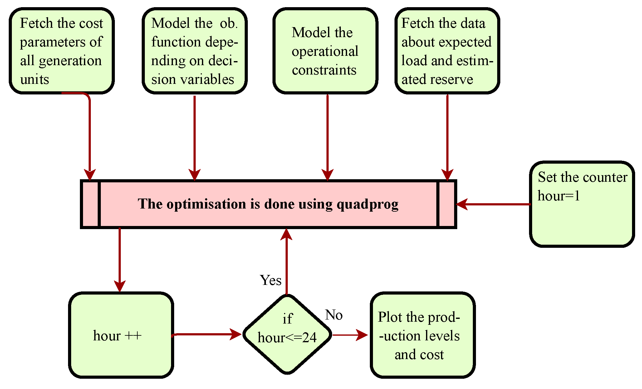
4. Simulation Methodology

In order to implement the proposed system, an IEEE 6 bus system connected to an electricity market is taken as a sample. There are n loads and three generation units, i.e., P 1 , P 2 , P 3 along with a windmill as RES. The fuel cost function F i is assumed to be a quadratic in accordance with production variables, which is given below:
F i = α P i 2 + β P i + γ i .
Equation (14) denotes a quadratic cost function that can be used for all thermal power generation facilities [63]. Such types of cost functions are optimally sized matrices, which depend upon fuel cost coefficients of respective energy generation units. Furthermore, the objective functions (Equations (1)–(4)) depict nonlinear mathematical model along with monotonic constraints, whereas all constraints exhibit a linear nature. The minimum and maximum limits on power generations and the values of other variables are given in Table 2, while total energy demand in each hour is presented in Table 3.
We can implement and perform optimization using the mathematical model discussed in the previous section by applying well known tools in order to get a numerical solution. MATLAB version 2017a (MathWorks Inc., Natick, MA, USA) on Macbook Pro, core i3 (Apple Inc., Cupertino, CA, USA) has been used for data handling, optimization and visualizing. The built-in quadprog solver has been selected due to its interior-point-convex and trust-region-reflective algorithms to solve the large scale nonlinear optimization problems.

5. Results

In this section, the simulation results in accordance with the test cases elaborated in Section 1.5 has been discussed. In case 1, the cost optimization for energy and reserve has been done separately. The objective function is formulated Equation (1). Figure 3 and Figure 4 show the energy consumption and cost profiles for all generation units over 24 h time, respectively. However, Figure 5 gives the energy and reserve capacity profile along with net demand, the net demand curve seems to be the same as the energy produced curve shifted upward. It can be assessed that demand is fulfilled by generation plus the energy retained as reserve which is kept at a constant value of 50 MW. The exaggerated peaks for both power and reserve give significant optimizing profiles as compared to those found in a real-time dispatch. Furthermore, the demand profile is also not significantly trending, leading to the most profound variations in power demand over the given time period. Because this profile has been chosen in order to reflect real-time consumption trends found in a daily life, regarding power generation, the high peaks are found during the evening due to industrial load and in the early morning due to residential usage. Similarly, low and medium peaks have been shown during other time intervals.
In case 2, energy generation facilities and reserve capacity are simultaneously co-dispatched to meet the power demand as explained in an objective function given in Equation (2). Figure 6 and Figure 7 show the energy consumption and cost profiles over the period of 24 h for case 2. At first glance, it seems that generation unit 3 is not contributing in providing power, as it is comparatively more expensive. Similarly, r 1 and r 2 are providing power due to their low cost as compared to r 3 , which is more costlier. Normally, the low cost energy generation facilities act as a “first choice”. This reserve capacity and high cost energy generation plants coming into operation for meeting the high or peak demand. This is due to fuel rates that have more exaggerated upward trend, making them infeasible to run during high demanding hours.
In case 3, energy and reserve is co-optimized considering a part of load which is not served, s . The mathematical model of this test case has been explained by the objective function given in Equation (3). Figure 8 and Figure 9 give the energy consumption and cost profiles in case 3. It is worth noting here that all power generation units are not working on their full rating and hence there is no power lost. In case a certain amount of power is not fulfilled due to an overload condition, then it is referred as under estimated load not served s , whereas s is a stochastic security measure that expresses the amount of demand not fulfilled as a result of load-shedding. It can happen due to many factors, i.e., economic loss to meet the demand or any fault at system. It is taken from the probability of uncertain factors and the involuntary loss on the system due to these events. In this research, s is taken as a linear value and included in a market-clearing problem. On the other hand, Figure 9 elucidates the cost profile of respective power generation units showing that only one reserve capacity unit is utilized because the reserve energy cost of other units is comparatively high.
In case 4, the energy and reserve capacity is co-optimized for a system with variable load, assuming two stochastic levels of load with 60% chances to be high and 40% to be on the low side. The mathematical model for this case has been explained with objective function given in Equation (4). Figure 10 gives the energy generation and load profiles in case 4 over the period of 24 h. The power generation and reserve energy allocated on each generation unit is shown for load demand at each hour of the day and the contribution of all resources to meet that demand. In Figure 11, the cost ($/h) for power production at each generation unit is shown for load demand at each hour of the day.
Case 5 has been modelled involving a wind power plant within the system discussed in previous cases. Now, load is served by RES on “first choice”. Then, the remaining load is satisfied by optimized dispatch of energy and reserve capacity. The wind power plant is modelled to produce power, based on the wind speed that is predicted using statistical data. The produced power is calculated using the formula given in Equation (5). The mathematical model is explained by the objective function given in Equation (4). Figure 12 shows the energy generation and load profiles in the presence of RES. This case demonstrates a stable energy generation profile instead of the fact that RES is available in a relatively small capacity. Here, the wind energy production charges have been neglected to permit its unimpeded utilization. Figure 13 shows the cost profile of power generation over the period of 24 h. The availability of relatively inexpensive reserve capacity leads lower generation from fuel operated power units during periods of high demand, thus bringing more economical cost. In total, 3.48% cost is saved due to renewable energy consideration. In Figure 14, the bar graph shows the energy generation from wind in the period of 24 h.
In case 6, the 14 bus model is considered with five generation units that has been taken from [69]. The energy generated and reserve capacity have been optimized for the demanded power in 24 h intervals. The results depict the same nature of findings as in case 3. The economic loss is also considered in the situation where some of the part of load is not served. Figure 15 shows the production levels of all generation units and amount of reserve incorporated to satisfy the load in each hour of the day. Figure 16 shows the cost profile of generation units and reserve capacity retained, and F s . As it is seen where the demand is at its peak values and being out of economic bounds, the F s is involved and a loss factor is associated with penalty of load not served.
Table 4 has the numerical details about the test cases implemented in this research. The load of 382 MW has been taken for numerical comparison between all cases. Cost has been reduced gradually in cases 1, 2 and 3 by improving the nature of the objective function. In case 4, the cost is slightly increased due to probabilistic approach for power demand to get more factual results. In case 5, the cost is reduced due to incorporation of RES. Case 6 has been implemented using a bigger network to further validate the application of proposed method. In this case, an increased number of generation units are operated at low cost comparatively. This is why the cost in this case is at a minimum as compared to other scenarios.

6. Conclusions

The proposed system has demonstrated the importance of reserve and wind energy to curtail the energy generation cost. For this purpose, a joint optimization algorithm has been used to simultaneously dispatch energy and reserve capacity in a day-ahead electricity market. The proposed system also has the capability to handle power loss uncertainty that is implemented in real-time test cases. To validate the effectiveness of the proposed mechanism, we have considered various test cases, where low cost energy and reserve facilities have been co-dispatched with improved economic efficiency. Nevertheless, these benefits are highly constrained due to generation, capacity, demand and process limits, whereas the incorporation of wind power model into the proposed approach helps to alleviate these constraints, and thus acts at the margin of maximal cost reduction. Furthermore, the proposed co-optimization program leads to understanding the observations that may not be radially apparent if each facility is developed separately. For example, the reserve and wind energy facilities in interconnected networks have additional benefits of shifting the generation from high peak hours to low peak hours. Hence, the results demonstrate that reserve and renewable resources have a particular role in a day-ahead electricity market.

Author Contributions

Conceptualization, M.W.H. and M.B.R.; methodology, M.B.R.; software, M.W.H.; validation, M.B.R., and M.W.H.; formal analysis, N.J.; investigation, N.J. and M.A.; resources, M.W.H.; data curation, M.W.H. and M.B.R.; writing—original draft preparation, M.W.H. and M.B.R.; writing—review and editing, N.J. and M.A.; visualization, N.J. and M.B.R.; supervision, M.B.R. and N.J.; project administration, M.B.R.; funding acquisition, The University of Lahore, Lahore, Pakistan.

Funding

This research received no external funding.

Acknowledgments

The authors would like to thank the Office of Research, Innovation and Commercialization (ORIC), The University of Lahore, Lahore, Pakistan for sponsoring this research.

Conflicts of Interest

The authors declare no conflict of interest.

Nomenclature

P i , g Electrical power generation from i th unit
P d Electrical power demand
x 0 Initial state for gradient search method
x 1 Next state for gradient search method
ϵ Convergence coefficient
F T Total cost
λ Incremental cost rate
Δ P Change in electrical power
P i min Minimum limit on i th energy generation unit
P i max Maximum limit on i th energy generation unit
S i min Minimum level of i th storage unit
S i max Maximum level of i th storage unit
r in Increase in energy for i th unit i = 1, 2, 3
R i Reserve capacity for i th unit allocated
r i Reserve capacity for i th unit utilized
e r Total reserve capacity
F r i Cost of reserve capacity for i th unit
F i Cost of running i th unit
s Amount of demand not served
τ H Probability factor for scenario High
τ L Probability factor for scenario Low
τ Probability factor
φ Power loss factor for economic load not served ( s = 0.05)
α Quadratic production cost function coefficient of i th power plant
β Linear production cost function coefficient of i th power plant
γ Constant production cost function coefficient of i th power plant
P w Electrical power generated from wind turbine
P R Rated electrical power of wind turbine
vWind speed
v c Cut-in wind speed
v R Rated wind speed
tTime horizon
NSet of energy generation units
L Lagrangian function

References

  1. Allan, R.N.; Billinton, R. Reliability Evaluation of Power Systems; Springer: New York, NY, USA, 2013. [Google Scholar]
  2. Wan, C.; Xu, Z.; Pinson, P. Direct Interval Forecasting of Wind Power. IEEE Trans. Power Syst. 2013, 28, 4877–4878. [Google Scholar] [CrossRef]
  3. Wan, C.; Xu, Z.; Pinson, P.; Dong, Z.Y.; Wong, K.P. Optimal Prediction Intervals of Wind Power Generation. IEEE Trans. Power Syst. 2014, 29, 1166–1174. [Google Scholar] [CrossRef] [Green Version]
  4. Salimi-Beni, A.; Fotuhi-Firuzabad, M.; Gharagozloo, H.; Farrokhzad, D. Impacts of load pattern variation in iran power system on generation system planning. In Proceedings of the Canadian Conference on Electrical and Computer Engineering, Saskatoon, SK, Canada, 1–4 May 2005; pp. 2216–2219. [Google Scholar] [CrossRef]
  5. Li, B.; Maroukis, S.D.; Lin, Y.; Mathieu, J.L. Impact of uncertainty from load-based reserves and renewables on dispatch costs and emissions. In Proceedings of the 2016 North American Power Symposium (NAPS), Denver, CO, USA, 18–20 September 2016; pp. 1–6. [Google Scholar]
  6. Stephenson, P.; Paun, M. Electricity market trading. Power Eng. J. 2001, 15, 277–288. [Google Scholar] [CrossRef]
  7. Morales, J.M.; Conejo, A.J.; Madsen, H.; Pinson, P.; Zugno, M. Integrating Renewables in Electricity Markets; Springer: Boston, MA, USA, 2014; pp. 57–100. [Google Scholar]
  8. Vîlceanu, R.C.; Chiosa, N.; Şurianu, F.D. Study of the load variation for an electrical consumer. In IOP Conference Series: Materials Science and Engineering; IOP Publishing: Bristol, UK, 2016; Volume 106, p. 012027. [Google Scholar]
  9. Barbulescu, C.; Kilyeni, S.; Deacu, A.; Turi, G.M.; Moga, M. Artificial neural network based monthly load curves forecasting. In Proceedings of the 2016 IEEE 11th International Symposium on Applied Computational Intelligence and Informatics (SACI), Timisoara, Romania, 12–14 May 2016; pp. 237–242. [Google Scholar]
  10. Kateeb, I.A.; Bikdash, M.; Chopade, P. Back to the future Renewable Energy Sources and green Smart Grid. In Proceedings of the 2011 Proceedings of IEEE Southeastcon, Nashville, TN, USA, 17–20 March 2011; pp. 147–152. [Google Scholar] [CrossRef]
  11. Ribeiro, H.; Unesco. Fossil fuel energy impacts on health. In Encyclopedia of Life Support Systems; Eolss Publishers Co.: Oxford, UK, 2001. [Google Scholar]
  12. Chen, C.; Wiser, R.; Mills, A.; Bolinger, M. Weighing the costs and benefits of state renewables portfolio standards in the United States: A comparative analysis of state-level policy impact projections. Renew. Sustain. Energy Rev. 2009, 13, 552–566. [Google Scholar] [CrossRef] [Green Version]
  13. Noskova, E.V.; Obyazov, V.A. Variations in wind parameters in the Zabaikal’skii krai. Russ. Meteorol. Hydrol. 2016, 41, 466–471. [Google Scholar] [CrossRef]
  14. Yan, Q.; Zhu, M.; Lin, W. Regional Variations of Wind Power and the Causes. Int. J. Simul. Syst. Sci. Technol. 2015, 16, 1–7. [Google Scholar]
  15. Jun, L. Study on the statistical characteristics of solar power. In IOP Conference Series: Earth and Environmental Science; IOP Publishing: Bristol, UK, 2017; Volume 52. [Google Scholar]
  16. Afolabi, L.O.; Adewunmi, O.T.; Seluwa, E.O.; Soliu-Salau, G.A.; Odeniyi, O.M. Prediction of solar radiation patterns for sustainable implementation of solar power generation. Ann. Fac. Eng. Hunedoara 2017, 15, 153–160. [Google Scholar]
  17. Solar Energy. Available online: https://en.wikipedia.org/wiki/Solarenergy (accessed on 9 March 2018).
  18. Wind Power Market to Reach 60 GW in 2018, Asia Keeps Lead. Available online: https://renewablesnow.com/news/wind-power-market-to-reach-60-gw-in-2018-asia-keeps-lead-471144 (accessed on 9 March 2018).
  19. Mishra, S.; Leinakse, M.; Palu, I. Wind power variation identification using ramping behavior analysis. Energy Procedia 2017, 141, 565–571. [Google Scholar] [CrossRef]
  20. Bajaj, S.; Sandhu, K.S. Wind turbine economics: A study. In Proceedings of the 2014 IEEE 6th India International Conference on Power Electronics (IICPE), Kurukshetra, India, 8–10 December 2014; pp. 1–5. [Google Scholar] [CrossRef]
  21. Premalatha, M.; Abbasi, T.; Abbasi, S.A. Wind energy: Increasing deployment, rising environmental concerns. Renew. Sustain. Energy Rev. 2014, 31, 270–288. [Google Scholar] [CrossRef]
  22. Walker, R.P.; Swift, A. Wind Energy Essentials: Societal, Economic, and Environmental Impacts; John Wiley & Sons: Hoboken, NJ, USA, 2015. [Google Scholar]
  23. Breton, S.P.; Moe, G. Status, plans and technologies for offshore wind turbines in Europe and North America. Renew. Energy 2009, 34, 646–654. [Google Scholar] [CrossRef]
  24. Parikh, M.M.; Bhattacharya, A.K. Wind data analysis for studying the feasibility of using windmills for irrigation. Energy Agric. 1984, 3, 129–136. [Google Scholar] [CrossRef]
  25. Han, X.S.; Gooi, H.B.; Kirschen, D.S. Dynamic economic dispatch: feasible and optimal solutions. IEEE Trans. Power Syst. 2001, 16, 22–28. [Google Scholar] [CrossRef]
  26. Castro, J.F.C.; da Silva, A.M.L.; Guaranys, B. Operating reserve requirements and equipment ranking in systems with renewable sources. In Proceedings of the 2018 Simposio Brasileiro de Sistemas Eletricos (SBSE), Niteroi, Brazil, 12–16 May 2018; pp. 1–6. [Google Scholar] [CrossRef]
  27. Contreras, J.; Asensio, M.; de Quevedo, P.M.; Muñoz-Delgado, G.; Montoya-Bueno, S. Joint RES and Distribution Network Expansion Planning under a Demand Response Framework; Elsevier Science: Amsterdam, The Netherlands, 2016; pp. 14–19. [Google Scholar]
  28. Song, Y.H. Operation of Market-Oriented Power Systems; Springer Science & Business Media: Berlin, Germany, 2003. [Google Scholar]
  29. Zhu, J. Optimization of Power System Operation; John Wiley & Sons: Hoboken, NJ, USA, 2015; Volume 47. [Google Scholar]
  30. Bayasgalan, Z.; Bayasgalan, T.; Muzi, F. Improvement of the dispatching preplanning process in day-ahead electricity market using a sequential method. In Proceedings of the 2017 18th International Conference on Computational Problems of Electrical Engineering (CPEE), Kutna Hora, Czech Republic, 11–13 September 2017; pp. 1–5. [Google Scholar] [CrossRef]
  31. Faqiry, M.N.; Zarabie, A.K.; Nassery, F.; Wu, H.; Das, S. A day-ahead market energy auction for distribution system operation. In Proceedings of the 2017 IEEE International Conference on Electro Information Technology (EIT), Lincoln, NE, USA, 14–17 May 2017; pp. 182–187. [Google Scholar] [CrossRef]
  32. Vasilj, J.; Jakus, D.; Sarajcev, P. Energy and reserve co-optimization in power system with wind and PV power. In Proceedings of the 2015 12th International Conference on the European Energy Market (EEM), Lisbon, Portugal, 19–22 May 2015; pp. 1–5. [Google Scholar] [CrossRef]
  33. Gan, D.; Litvinov, E. Energy and reserve market designs with explicit consideration to lost opportunity costs. IEEE Trans. Power Syst. 2003, 18, 53–59. [Google Scholar] [CrossRef]
  34. Santhosh, A.; Farid, A.M.; Youcef-Toumi, K. Real-time economic dispatch for the supply side of the energy-water nexus. Appl. Energy 2014, 122, 42–52. [Google Scholar] [CrossRef]
  35. Santra, D.; Mondal, A.; Mukherjee, A. Study of economic load dispatch by various hybrid optimization techniques. In Hybrid Soft Computing Approaches; Springer: New Delhi, India, 2016; pp. 37–74. [Google Scholar]
  36. Thenmalar, K.; Allirani, A. Optimization Techniques for the Economic Dispatch Problem in Various Generation Plant. Adv. Mater. Res. 2013, 768, 323–328. [Google Scholar] [CrossRef]
  37. Sivanagaraju, S. Power System Operation and Control; Pearson Education India: New Delhi, India, 2009. [Google Scholar]
  38. Sönmez, Y. Estimation of fuel cost curve parameters for thermal power plants using the ABC algorithm. Turk. J. Electr. Eng. Comput. Sci. 2013, 21, 1827–1841. [Google Scholar] [CrossRef]
  39. Helseth, A.; Fodstad, M.; Mo, B. Optimal Medium-Term Hydropower Scheduling Considering Energy and Reserve Capacity Markets. IEEE Trans. Sustain. Energy 2016, 7, 934–942. [Google Scholar] [CrossRef]
  40. Wang, Z.; Negash, A.; Kirschen, D.S. Optimal scheduling of energy storage under forecast uncertainties. IET Gener. Transm. Distrib. 2017, 11, 4220–4226. [Google Scholar] [CrossRef]
  41. Li, Y.Z.; Zhao, T.; Wang, P.; Gooi, H.B.; Wu, L.; Liu, Y.; Ye, J. Optimal Operation of Multi-Microgrids via Cooperative Energy and Reserve Scheduling. IEEE Trans. Ind. Inform. 2018, 14, 3459–3468. [Google Scholar] [CrossRef]
  42. Cobos, N.G.; Arroyo, J.M.; Alguacil-Conde, N.; Wang, J. Robust Energy and Reserve Scheduling Considering Bulk Energy Storage Units and Wind Uncertainty. IEEE Trans. Power Syst. 2018, 33, 5206–5216. [Google Scholar] [CrossRef]
  43. Tan, Y.T.; Kirschen, D.S. Co-optimization of Energy and Reserve in Electricity Markets with Demand-side Participation in Reserve Services. In Proceedings of the 2006 IEEE PES Power Systems Conference and Exposition, Atlanta, GA, USA, 29 October–1 November 2006; pp. 1182–1189. [Google Scholar] [CrossRef]
  44. Karangelos, E.; Bouffard, F. Towards Full Integration of Demand-Side Resources in Joint Forward Energy/Reserve Electricity Markets. IEEE Trans. Power Syst. 2012, 27, 280–289. [Google Scholar] [CrossRef]
  45. Ehsani, A.; Ranjbar, A.M.; Fotuhi-Firuzabad, M. A proposed model for co-optimization of energy and reserve in competitive electricity markets. Appl. Math. Model. 2009, 33, 92–109. [Google Scholar] [CrossRef]
  46. Al-Roomi, A.R.; El-Hawary, M.E. A novel multiple fuels’ cost function for realistic economic load dispatch needs. In Proceedings of the 2017 IEEE Electrical Power and Energy Conference (EPEC), Saskatoon, SK, Canada, 22–25 October 2017; pp. 1–6. [Google Scholar]
  47. Abido, M.A. Environmental/economic power dispatch using multiobjective evolutionary algorithms. IEEE Trans. Power Syst. 2003, 18, 1529–1537. [Google Scholar] [CrossRef]
  48. Shalini, S.P.; Lakshmi, K. Solving Environmental Economic Dispatch Problem with Lagrangian Relaxation Method. Int. J. Electron. Electr. Eng. 2014, 7, 9–20. [Google Scholar]
  49. Mohatram, M. Hybridization of artificial neural network and lagrange multiplier method to solve economic load dispatch problem. In Proceedings of the 2017 International Conference on Infocom Technologies and Unmanned Systems (Trends and Future Directions) (ICTUS), Dubai, UAE, 18–20 December 2017; pp. 514–520. [Google Scholar]
  50. Joya, G.; Atencia, M.A.; Sandoval, F. Hopfield neural networks for optimization: study of the different dynamics. Neurocomputing 2002, 43, 219–237. [Google Scholar] [CrossRef]
  51. Santra, D.; Mukherjee, A.; Sarker, K.; Mondal, S. Medium scale multi-constraint economic load dispatch using hybrid metaheuristics. In Proceedings of the 2017 Third International Conference on Research in Computational Intelligence and Communication Networks (ICRCICN), Kolkata, India, 3–5 November 2017; pp. 169–173. [Google Scholar]
  52. Gautham, S.; Rajamohan, J. Economic load dispatch using novel bat algorithm. In Proceedings of the 2016 IEEE 1st International Conference on Power Electronics, Intelligent Control and Energy Systems (ICPEICES), Delhi, India, 4–6 July 2016; pp. 1–4. [Google Scholar]
  53. Babu, B. Self Adaptive Firefly Algorithm for Economic Load Dispatch. Int. J. Eng. Trends Technol. 2017, 48, 110–115. [Google Scholar] [CrossRef]
  54. Alsumait, J.S.; Sykulski, J.K.; Al-Othman, A.K. A hybrid GA–PS–SQP method to solve power system valve-point economic dispatch problems. Appl. Energy 2010, 87, 1773–1781. [Google Scholar] [CrossRef] [Green Version]
  55. dos Santos Coelho, L.; Mariani, V.C. An improved harmony search algorithm for power economic load dispatch. Energy Convers. Manag. 2009, 50, 2522–2526. [Google Scholar] [CrossRef]
  56. Lingala, R.; Bethina, A.; Rao, P.R.; Sumanth, K. Economic load dispatch using heuristic algorithms. In Proceedings of the 2015 IEEE International WIE Conference on Electrical and Computer Engineering (WIECON-ECE), Dhaka, Bangladesh, 19–20 December 2015; pp. 519–522. [Google Scholar] [CrossRef]
  57. Chiang, C.L. Genetic algorithm for power load dispatch. In Proceedings of the 2008 IEEE Conference on Cybernetics and Intelligent Systems, Chengdu, China, 21–24 September 2008; pp. 347–352. [Google Scholar] [CrossRef]
  58. Chellappan, R.; Kavitha, D. Economic and emission load dispatch using Cuckoo search algorithm. In Proceedings of the 2017 Innovations in Power and Advanced Computing Technologies (i-PACT), Vellore, India, 21–22 April 2017; pp. 1–7. [Google Scholar] [CrossRef]
  59. Gaing, Z.L. Particle swarm optimization to solving the economic dispatch considering the generator constraints. IEEE Trans. Power Syst. 2003, 18, 1187–1195. [Google Scholar] [CrossRef] [Green Version]
  60. Dzobo, O.; Shehata, A.M.; Azimoh, C.L. Optimal economic load dispatch in smart grids considering uncertainty. In Proceedings of the 2017 IEEE AFRICON, Cape Town, South Africa, 18–20 September 2017; pp. 1277–1282. [Google Scholar] [CrossRef]
  61. Shahinzadeh, H.; Fathi, S.H.; Moazzami, M.; Hosseinian, S.H. Hybrid Big Bang-Big Crunch Algorithm for solving non-convex Economic Load Dispatch problems. In Proceedings of the 2017 2nd Conference on Swarm Intelligence and Evolutionary Computation (CSIEC), Kerman, Iran, 7–9 March 2017; pp. 48–53. [Google Scholar]
  62. Coelho, L.S.; Mariani, V.C. Combining of chaotic differential evolution and quadratic programming for economic dispatch optimization with valve-point effect. IEEE Trans. Power Syst. 2006, 21, 989–996. [Google Scholar] [CrossRef]
  63. Wood, A.J.; Wollenberg, B.F. Power Generation, Operation, and Control; John Wiley & Sons: Hoboken, NJ, USA, 2012. [Google Scholar]
  64. Park, J.H.; Kim, Y.S.; Eom, I.K.; Lee, K.Y. Economic load dispatch for piecewise quadratic cost function using hopfield neural network. IEEE Trans. Power Syst. 1993, 8, 1030–1038. [Google Scholar] [CrossRef]
  65. Kies, A.; Schyska, B.U.; von Bremen, L. Curtailment in a Highly Renewable Power System and Its Effect on Capacity Factors. Energies 2016, 9, 510. [Google Scholar] [CrossRef]
  66. Chang, Y.C.; Yang, W.T.; Liu, C.C. A new method for calculating loss coefficients of power systems. IEEE Trans. Power Syst. 1994, 9, 1665–1671. [Google Scholar] [CrossRef]
  67. Zhang, X.; Zhang, B. Equal incremental rate economic dispatching and optimal power flow for the union system of microgrid and external grid. In Proceedings of the 2014 IEEE PES General Meeting Conference & Exposition, National Harbor, MD, USA, 27–31 July 2014. [Google Scholar]
  68. Elanchezhian, E.B.; Subramanian, S.; Ganesan, S. Economic power dispatch with cubic cost models using teaching learning algorithm. IET Gener. Transm. Distrib. 2014, 8, 1187–1202. [Google Scholar] [CrossRef]
  69. Appendix A: DATA SHEETS FOR IEEE 14 BUS SYSTEM. Available online: https://www.researchgate.net/profile/Mohamed_Mourad_Lafifi/post/-\Datasheet_for_5_machine_14_bus_ieee_system2/attachment/59d637fe\79197b8077995409/AS%3A395594356019200%401471328452063/\download/DATA+SHEETS+FOR+IEEE+14+BUS+SYSTEM+19_\appendix.pdf (accessed on 9 March 2018).
Figure 1. Flowchart of the proposed system.
Energies 11 02833 g001
Figure 2. Sample demand profile for a domestic consumption over the period of 24 h.
Energies 11 02833 g002
Figure 3. Power generation and demand profile of different generation unit over the time of 24 h (case 1).
Energies 11 02833 g003
Figure 4. Total cost obtained by different units to fulfill demand over the time of 24 h (case 1).
Energies 11 02833 g004
Figure 5. Relationship between energy and reserve capacity over the time of 24 h (case 1).
Energies 11 02833 g005
Figure 6. Power generation and demand profile of different generation units over the time of 24 h (case 2).
Energies 11 02833 g006
Figure 7. Total cost obtained by different units to fulfill demand over the time of 24 h (case 2).
Energies 11 02833 g007
Figure 8. Power generation and demand profile of different generation units over the time of 24 h (case 3).
Energies 11 02833 g008
Figure 9. Total cost obtained by different units to fulfill demand over the time of 24 h (case 3).
Energies 11 02833 g009
Figure 10. Power generation and demand profile of different generation units over the time of 24 h (case 4).
Energies 11 02833 g010
Figure 11. Total cost obtained by different units to fulfill demand over the time of 24 h (case 4).
Energies 11 02833 g011
Figure 12. Power generation and demand profile of different units along with renewable energy unit to fulfill demand over the time of 24 h (case 5).
Energies 11 02833 g012
Figure 13. Total cost obtained by different units to fulfill demand over the time of 24 h (case 5).
Energies 11 02833 g013
Figure 14. Wind energy variations over the time of 24 h (case 5).
Energies 11 02833 g014
Figure 15. Power generation and demand profile of different units along with renewable energy unit to fulfill demand over the time of 24 h (case 6).
Energies 11 02833 g015
Figure 16. Total cost obtained by different units to fulfill demand over the time of 24 h (case 6).
Energies 11 02833 g016
Table 1. Comparison of related work.
Ref.Techniques UsedObjectivesLimitationsRESReserve
C. Barbulescu et al. [9]Artificial Neural Network (ANN)To estimate the monthly load curvesPrevious data required on a large scaleX
S. Mishra et al. [19]Ramping behavior analysisTo study wind power variationsOnly significant variations are involvedX
A. Helseth et al. [39]Stochastic dynamic programmingTo optimally schedule the hydro-power generation unitsLinearisation of expressions may lead to inaccurate commitment schedulingX
Z. Wang et al. [40]Two stage optimization modelTo dispatch electrical power optimally involving PV forecastingOperational cost of storage units are not consideredX
Y. Z. Li et al. [41]Cooperative model of energy and reserve capacityTo design a model for multi-micro grids involving energy and reserve capacityRobust optimization is a conservative method
G. Noemi et al. [42]Novel two-stage robust optimizationCo-optimized electricity market of energy and reserve capacity involving wind uncertaintyLack of non-spinning reserve
Y. T. Tan et al. [43]Mixed integer programmingCo-optimized electricity market of energy and reserve capacity considering demand sideLack of quadratic nature of cost curves
M. A. Abido et al. [47]Strength pareto evolution algorithmTo solve Economic Load Dispatch (ELD) involving environmental constraintsSecurity and stability parameters are not involvedXX
M. Mohatram et al. [49]Hybrid ANN & Lagrange Multiplier Method (LMM)To improve the results of ELD by using non traditional methodIn case of more generation units, system complexity may increaseXX
S. Gautham et al. [52]Novel Bat Algorithm (NBA)To improve the results of ELD by using non traditional methodConvergence time is more due to large number of variable involvedXX
Babu et al. [53]Self Adaptive Firefly Algorithm (SA-FA)To improve the results of ELD involving valve point effect by using non traditional methodSystem complexity increases wiht the increase in system variablesXX
D. Santra et al. [51]Hybrid Particle Swarm Optimization (PSO) & Ant Colony Optimization (ACO) algorithmTo solve ELD problem involving transmission losses, ramp rate function and valve point effectLess optimal results have been produced due to traditional techniquesXX
Alsumait et al. [54]Hybrid Genetic Algorithm (GA) & PSO & Sequential Quadratic Programming (SQP)To solve ELD problem involving valve point effectThis algorithm is not suitable for small networks as compared with other methods and also reserve capacity is not retainedXX
L. dos Santos et al. [51]Improved harmony search algorithmTo solve ELD involving valve point effectgeneration units has not applied with non operating zones and also reserve capacity is not retainedXX
O. Dzobo et al. [60]Quadratic programmingTo solve ELD considering uncertainty at the generation endVery limited number of constraints appliedX
Zwe-Lee Gaing et al. [59]PSOTo improve the results of ELD by using non traditional methodLess optimal results are found as compared to non-conventional techniquesXX
H. Shahinzadeh et al. [61]Hybrid Big Bang–Big Crunch(BB–BC) algorithmTo solve Non Convex ELD problemAlgorithm requires large number iterations to find optimal solutionXX
L. S. Coelho et al. [62]Hybrid (Chaotic differential algorithm & Quadratic programming)To solve Non convex ELD problemMore decision and system variable may increase system complexityXX
J. H. Park et al. [64]Hopfield Neural Network (HNN)ELD for piecewise quadratic cost curvesAlgorithm works only for piecewise cost functions also reserve capacity is not retainedXX
Table 2. Operating limits of generation units [68].
Generation UnitIndexMinimum Production (MW)Maximum Production (MW)Reserve Energy Cost ($)Power Plant Cost Coefficients
α β γ
P G 1 i 1 50200201.070 × 10 2 1.1699 × 10 + 1 213
P G 2 i 2 37.5150151.780 × 10 2 1.0113 × 10 + 1 200
P G 3 i 3 45180221.480 × 10 2 1.0883 × 10 + 1 240
Table 3. Total power demand for 24 h.
Time (HRS)12 a.m.1 a.m.2 a.m.3 a.m.4 a.m.5 a.m.
Load (MW)382409490374510480
Time (HRS)6 a.m.7 a.m.8 a.m.9 a.m.10 a.m.11 a.m.
Load (MW)443457405439515452
Time (HRS)12 p.m.1 p.m.2 p.m.3 p.m.4 p.m.5 p.m.
Load (MW)448404443464472429
Time (HRS)6 p.m.7 p.m.8 p.m.9 p.m.10 p.m.11 p.m.
Load (MW)425519375503507490
Table 4. Numerical results of all test cases implemented.
CaseLoad (MW)Reserve Capacity (MW)Renewable Generation (MW)Total Cost ($/MW)
138250X6308
238250X6293
338250X6319
438250X6334.2
5382506138.0
638250X1786.2

