An Optimal and Distributed Demand Response Strategy for Energy Internet Management

Abstract

This study proposes a new model of demand response management for a future smart grid that consists of smart microgrids. The microgrids have energy storage units, responsive loads, controllable distributed generation units, and renewable energy resources. They can buy energy from the utility company when the power generation in themselves cannot satisfy the load demand, and sell extra power generation to the utility company. The goal is to optimize the operation schedule of microgrids to minimize the microgrids’ payments and the utility company’s operation cost. A parallel distributed optimization algorithm based on games theory is developed to solve the optimization problem, in which microgrids only need to send their aggregated purchasing/selling energy to the utility company, thus avoid infringing its privacy. Microgrids can update their operation schedule simultaneously. A case study is implemented, and the simulation results show that the proposed method is effective and efficient.

1. Introduction

The current electric power system that uses fossil fuels, e.g., oil, coal, and natural gas as energy resources, has been serving us for more than five decades [1]. However, these fossil fuels are being consumed rapidly. The resultant energy crisis and environmental pollution problems have attracted more and more attention to finding alternative energy resources that are sustainable and environmental friendly [2].

The next-generation electric power system, i.e., the smart grid, is conceived of as an electric grid that integrates the actions of all users connected to it and makes use of advanced information, control, and communication technologies to save energy, reduce cost, and increase reliability and transparency [3]. In order to reduce the operation complexity of the smart grid, the promising concept, the microgrid, is proposed [4].

A typical microgrid is a small scaled power grid that comprises energy storage units, e.g., battery and electric capacity; controllable distributed generators, e.g., micro-turbine and diesel, which are dispatchable units; renewable energy resources, e.g., wind and solar, which are non-controllable devices; and smart loads, which comprise curtailable loads, schedulable loads, and critical loads. The curtailable loads can be shed when there is an emergent situation, and the schedulable loads can be shiftable when it is convenient [5,6]. There are two frequently used modes of operation in a microgrid, i.e., the grid-connected mode and the isolated mode. In the grid-connected mode, the microgrid can purchase from/sell power to the utility company. Therefore, the microgrid can play a very important role in the demand response programs of the smart grid.

Demand-side management involves optimal operations of various power generation units, loads, etc., and it is now receiving more and more attention. It is a portfolio of strategies to improve the energy system at the side of consumption. In 2011, Palensky and Dietrich [7] provide an overview and a taxonomy for demand-side management (demand response, intelligent energy systems, and smart loads) in which various types of demand-side management are discussed.

The principal goal of demand response is to reduce the generation cost of utility company by reducing the peak load and shifting peak-load hours to off-peak hours [8]. In the traditional electricity market, the demand response program is implemented by considering time-of-use pricing. The price is fixed for a relatively long period, and the load schedule of users are not considered [9,10]. In the smart grid condition, the advanced metering infrastructure and high reliable communication network enable communication between the utility company and the microgrid users. Also, the real-time pricing based demand response programs can be used.

In [11], a demand response strategy is proposed to minimize the building energy payment by scheduling the appliances in a real-time electricity pricing condition. In [12], a distributed algorithm for control and coordination of loads and distributed energy resources in distribution networks is discussed; however, the interaction between the consumers and the electricity price is not considered. In [13], a parallel autonomous optimization scheme is proposed for demand response in smart grid. In [14], a demand response management strategy for plug-in electric vehicles and renewable energy resources is discussed. However, most of studies only considered a part of the units in the smart grid, such as the smart loads in [13] and plug-in electric vehicles in [14]. In [15,16], a mathematical model of a direct current microgrid supplied with photovoltaic and wind power generation, storage (battery bank), and a conventional power grid is presented. With the model, the voltage management strategy is implemented and analyzed.

Ou and Hong [17] investigated dynamic operation and control strategies for a microgrid hybrid wind-PV-FC based power supply system. In their study, an intelligent controller consists of an RBFNSM (radial basis function network-sliding mode), and a GRNN (General Regression Neural Network) for MPPT (maximum power point tracking) control is developed to achieve a fast and stable response for real power control.

Ou et al. [18] also proposed a hybrid bird-mating optimization approach to connection decisions of distribution transformers. The aim is to mitigate the voltage imbalance and deviation, ensuring a satisfactory supplying power. In [19], the authors applied a novel intelligent damping controller for the static synchronous compensator to reduce the power fluctuations, voltage support, and damping in a hybrid power multi-system. Experimental results show that the proposed controller is able to achieve better damping characteristics and effectively stabilize the network even under unstable conditions. In [20], the issue of load management in a microgrid is studied. A self-decision-making method based on the multi-agent system theory is proposed, and is shown as being effective at reducing peak load. By using a multi-agent system, in [21], automatic reconfiguration of microgrids is studied once a new device is added or a change is detected in the operation status of an existing device. There are also studies investigating the properties of microgrids from the perspective of agent system. For a comprehensive review of such studies, please refer to [22].

Haider et al. [23] proposed a new demand response scheme based on an adaptive consumption level pricing scheme. The proposed scheme is shown to be superior to block tariff and time-of-use price schemes. In the proposed scheme, customers are encouraged to manage the energy consumption and consequently lower their energy bill. The utilities are allowed to manage the aggregate consumption and predict the load requirement.

In [24], a multi-objective model is proposed for achieving an optimal demand response programing. The model aims to minimize the overall energy consumption and meanwhile to improve the technical parameter of the microgrid. The artificial bee colony algorithm and quasi-static technique are utilized to solve the model. Although considering the problem as a multi-objective is interesting, the selection of a satisfied Pareto optimal solution is not easy.

In addition to studies of optimal operation of microgrids, Ou [25] developed a simple yet effective unsymmetrical faults analysis method with hybrid compensation for microgrid (MG) distribution systems. Subsequently, the author proposed a direct building algorithm for microgrid distribution ground fault analysis [26]. Moreover, in [26], the authors discussed the ground fault model of a battery energy storage system as a distributed energy resource.

In this paper, we propose a demand response strategy for the microgrids in a smart grid condition, where the microgrid can purchase power from the utility company if the generation in it cannot satisfy the load demand and sell surplus power back to the utility company as well. The power generation of the utility and the real-time electricity price are both determined by the aggregation of microgrids. The operation of the dispatchable units is optimized by the energy management system (EMS) of the microgrid according to the updated price information and system state of the microgrid. The aggregated operation scheme of a microgrid in each iteration is sent to the utility company by the advanced metering infrastructure. Lastly, a case study is presented to demonstrate the efficiency and effectiveness of the proposed method.

The rest of this study is organized as follows: Section 2 provides the brief problem formulation; Section 3 introduces the distributed optimal energy management algorithm; simulation and results are shown in Section 4; Section 5 presents the conclusions.

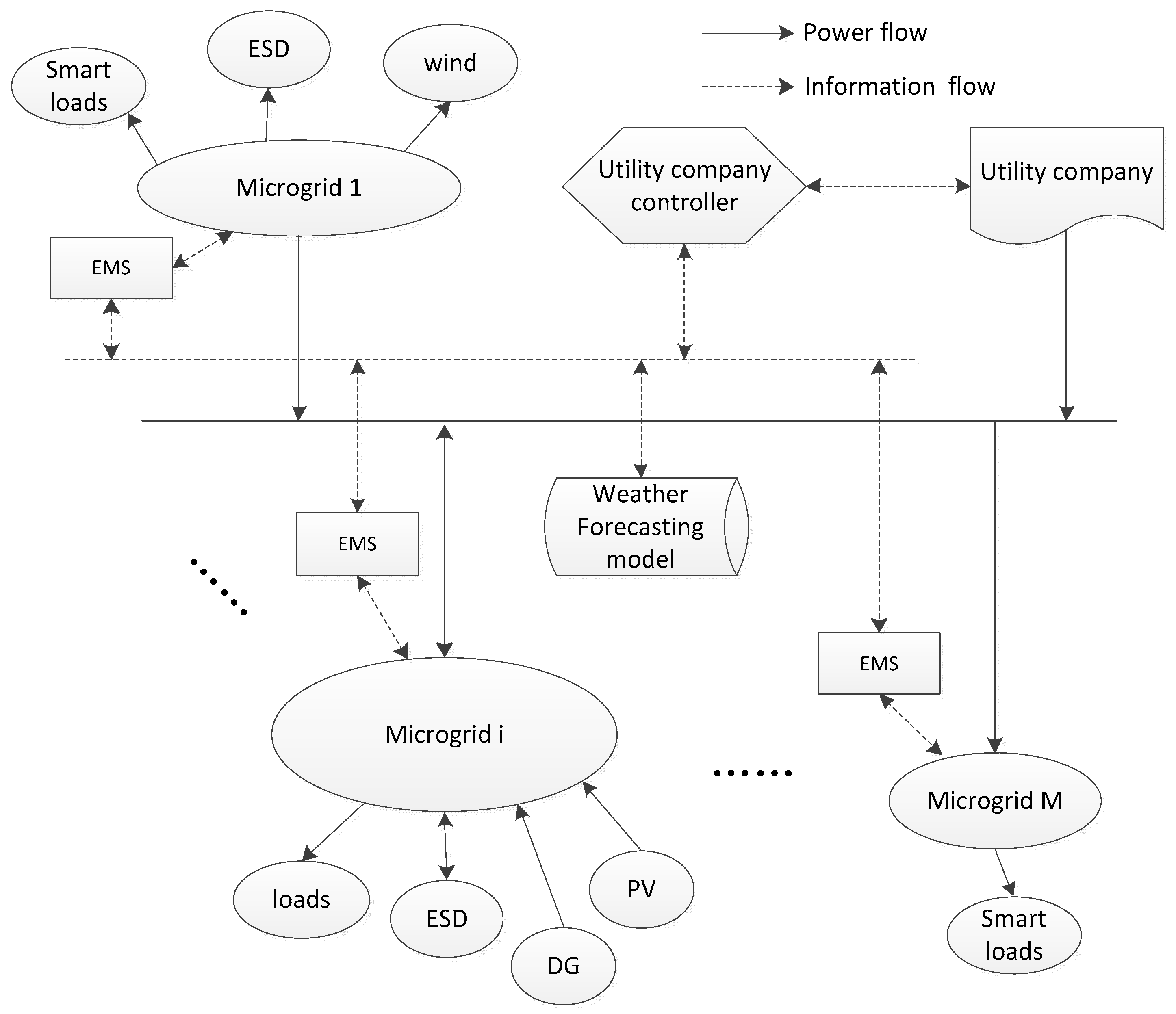
2. Problem Formulation

The basic structure of the smart grid is shown as Figure 1. It comprises several microgrid users. Some users only have smart loads, some users have no energy storage devices (ESDs), some users have no renewable energy sources (RESs), and other users have no controllable distributed generation (CDGs). The weather forecasting model collects the weather data of this area and predicts the needed data, such as wind speed, solar radiation, and load demand, and broadcasts this information to each microgrid user and the utility company controller. Smart metering devices measure the consumption of electricity, RESs generation, CDG generation, and ESD energy level in each microgrid. The EMS of each individual microgrid is responsible for optimizing the operation routines of dispatchable units in the microgrid to minimize the operation costs of its microgrid. The utility company controller receives the aggregates purchasing/selling power of each microgrid and schedule the generation plan of the generation units to minimize the costs of the utility company and broadcast the real-time electricity price to all the microgrids. In addition, the two-way communication between the microgrid EMS and the utility company controller is enabled.

The mathematical formulations of the optimal demand response problem of microgrids in a smart grid condition are shown as follows.

The essential work of the utility company is to satisfy the power demand of the smart grid in each time interval, i.e.,

$${\displaystyle \sum _{i=1}^M}\left(P_{i,gridI}\left(t\right)-P_{i,gridI}\left(t\right)\right)=P_{utility}\left(t\right)$$

(1)

where $t\in \left[1,T\right]$, and $T$ is the control and prediction horizon. $M$ is the amount of microgrids included in the smart grid system. $P_{i,gridI}\left(t\right)$, $P_{i,gridI}\left(t\right)$ are the purchasing and selling power of microgrid $i$ in time interval $t$, respectively, and $P_{utility}\left(\mathrm{t}\right)$ denotes the generation of the utility company in time interval $t$.

The generation of the utility company must be bounded by the system limit:

$$0\le P_{utility}\left(t\right)\le P_{utility}^{max}$$

(2)

$$-R_{utility}\left(t\right)\le P_{utility}\left(t\right)-P_{utility}\left(t-1\right)\le R_{utility}\left(t\right)$$

(3)

where $t\in \left[1,T\right]$. $P_{utility}^{max}$, $R_{utility}\left(t\right)$ are the maximum power generation and maximum ramp up/down power of the utility.

According to the rate-of-return regulations [13,15], the utility company can earn a fair revenue. Therefore, the real-time electricity price in present paper can be expressed as follows,

$$p_{buy}\left(t\right)=\phi \left(t\right)\frac{C\left(P_{utility}\left(t\right)\right)}{P_{utility}\left(t\right)}$$

(4)

$$p_{sell}\left(t\right)=\frac{C\left(P_{utility}\left(t\right)\right)}{P_{utility}\left(t\right)}$$

(5)

where $\phi \left(t\right),t\in \left[1,T\right]$ is the rate-of-return parameter of the utility company, its amount is determined by the coordination among the utility company, microgrid user, and the government organization. $C\left(P_{utility}\left(t\right)\right)$ indicates the operation cost of the utility company when its generation power is $P_{utility}\left(t\right)$. $p_{buy}\left(t\right)$, $p_{sell}\left(t\right)$ are the purchasing and selling power price for the microgrid users.

As the purchasing and selling power price are often different at the same time, the power interaction model between the $i\mathrm{th}$ microgrid and the utility company are modified as follows,

$$P_{i,gridI}^{min}{\delta }_{i,gridI}\left(t\right)\le P_{i,gridI}\left(t\right)\le P_{i,gridI}^{max}{\delta }_{i,gridI}\left(t\right)$$

(6)

$$P_{i,gridI}^{min}{\delta }_{i,gridI}\left(t\right)\le P_{i,gridO}\left(t\right)\le P_{i,gridO}^{max}{\delta }_{i,gridO}\left(t\right)$$

(7)

$${\delta }_{i,gridI}\left(t\right)+{\delta }_{i,gridO}\left(t\right)\le 1$$

(8)

where $t\in \left[1,T\right]$, $i\in \left[1,M\right]$. $P_{i,gridI}^{min}$, $P_{i,gridI}^{max}$ are the minimum, maximum purchasing power limit for the $i\mathrm{th}$ microgrid, respectively. Correspondingly, $P_{i,gridO}^{min}$, $P_{i,gridO}^{max}$ are the minimum, maximum selling power limit for the $i\mathrm{th}$ microgrid, respectively. ${\delta }_{i,gridI}\left(t\right)$, ${\delta }_{i,gridO}\left(t\right)$ are the purchasing, selling statuses of the $i\mathrm{th}$ microgrid in time interval $t$, respectively.

Equations (6) and (7) are the purchasing and selling power limits, respectively, and Equation (8) is the purchasing and selling action constraints, as a microgrid cannot purchase and sell power at the same time.

For each microgrid, it must satisfy the supply and demand balance in every time interval, i.e.,

$$P_{i,gridI}\left(t\right)+P_{i,CDG}\left(t\right)+P_{i,Ed}\left(t\right)+P_{i,wind}\left(t\right)+P_{i,PV}\left(t\right)=P_{i,Ec}\left(t\right)+l_{i,load}\left(t\right)+P_{i,gridO}\left(t\right);$$

(9)

where $t\in \left[1,T\right]$, $i\in \left[1,M\right]$. $P_{i,CDG}\left(t\right)$, $P_{i,wind}\left(t\right)$, $P_{i,PV}\left(t\right)$ are the generation of CDG units, wind farms, and PV plants in the microgrid, respectively. $P_{i,Ed}\left(t\right)$, $P_{i,Ec}\left(t\right)$ are the discharging and charging power of the ESD units, respectively. $l_{i,load}\left(t\right)$ is the aggregated load demand of this microgrid. It is worth mentioning that not all microgrids have all the elements in Equation (9)—some microgrids only have part of the elements.

Similar to the generators in the utility company, the CDG unit in this study is bounded as follows.

$$P_{i,CDG}^{min}{\delta }_{i,CDG}\left(t\right)\le P_{i,CDG}\left(t\right)\le {\delta }_{i,CDG}\left(t\right)P_{i,CDG}^{max}$$

(10)

$$-R_{i,CDG}\left(t\right)\le P_{i,CDG}\left(t\right)-P_{i,CDG}\left(t-1\right)\le R_{i,CDG}\left(t\right)$$

(11)

where $t\in \left[1,T\right]$, $i\in \left[1,M\right]$. $P_{i,CDG}^{min}$, $P_{i,CDG}^{max}$ are the minimum and maximum power generation of the CDG units, and $R_{i,CDG}\left(t\right)$ is the ramp up/down power of the CDG units.

The ESD units in the microgrid play an important role in the system planning and scheduling. They can discharge power during high price hours and charge power during low price hours to make money, and can act as a backup when dealing with emergency conditions. The operation of the ESD units should satisfy the energy level, charging power, discharging power, operation status, and dynamic model constraints. i.e.,

$$E_{i,E}^{min}\le E_{i,E}\left(t+1\right)\le E_{i,E}^{max}$$

(12)

$${\delta }_{i,Ec}\left(t\right)P_{i,Ec}^{min}\le P_{i,Ec}\left(t\right)\le {\delta }_{i,Ec}\left(t\right)P_{i,Ec}^{max}$$

(13)

$${\delta }_{i,Ed}\left(t\right)P_{i,Ed}^{min}\le P_{i,Ed}\left(t\right)\le {\delta }_{i,Ed}\left(t\right)P_{i,Ed}^{max}$$

(14)

$${\delta }_{i,Ec}\left(t\right)+{\delta }_{i,Ed}\left(t\right)\le 1$$

(15)

$$E_{i,E}\left(t+1\right)=E_{i,E}\left(t\right)+\left({\eta }_{i,Ec}{P}_{i,Ec}\left(t\right)-1/{\eta }_{i,Ed}{P}_{i,Ed}\left(t\right)\right)∆t-{\epsilon }_{i,E}$$

(16)

where $t\in \left[1,T\right]$, $i\in \left[1,M\right]$. $E_{i,E}\left(t\right)$ denotes ESD unit energy level of the $i\mathrm{th}$ microgrid in period $t$. ${\eta }_{i,Ec}$, ${\eta }_{i,Ed}$, ${\epsilon }_{i,E}$ are the charge efficiency, discharge efficiency, and self-discharge loss of the ESD unit in the $i\mathrm{th}$ microgrid, respectively. $P_{i,Ec}^{min}$, $P_{i,Ec}^{max}$ are the minimum and maximum charging power, respectively. Also, $P_{i,Ed}^{min}$, $P_{i,Ed}^{max}$ are the minimum and maximum discharging power, respectively.

Equation (14) is the energy level constraint, and Equations (15) and (16) are the charging and discharging power constraints, respectively. Equation (17) is the charging/discharging operation status constraint, because the ESD unit cannot charge and discharge at the same time. Equation (18) is the dynamic model of the ESD unit. The ESD unit model presented in this paper can effectively express the hybrid dynamic feature of the energy storage without introducing extra auxiliary variables and extra models.

The loads in the $i\mathrm{th}$ microgrid include critical loads, schedulable loads, and flexible loads [27]. Therefore, the load demand in microgrid $i$ can be denoted as follows,

$$l_{i,load}\left(t\right)=l_{i,cri}\left(t\right)+l_{i,F}\left(t\right)\left(1-{\theta }_{i,F}\left(t\right)\right)+{\displaystyle \sum _{a=1}^{A_{i,S}}}{l}_{i,a}\left(t\right)$$

(17)

where $t\in \left[1,T\right]$, $i\in \left[1,M\right]$. $l_{i,cri}\left(t\right)$, $l_{i,F}\left(t\right)$ are the forecasted critical load demand and curtaillable load demand, respectively. ${\theta }_{i,F}\left(t\right)$ is the power curtailment ratio of the $i\mathrm{th}$ microgrid in time interval $t$. $A_{i,S}$ is the set of schedulable appliances of the $i\mathrm{th}$ microgrid, and $l_{i,a}\left(t\right)$ is the load demand of appliance $\mathrm{a}$ of the $i\mathrm{th}$ microgrid in time interval $t$. The detailed constraints are shown as follows,

$$0\le {\theta }_{i,F}\left(t\right)\le {\theta }_{i,F}^{max}$$

(18)

$$0\le l_{i,F}\left(t\right)\le l_{i,F}^{max}$$

(19)

$$0\le l_{i,cri}\left(t\right)\le l_{i,cri}^{max}$$

(20)

$$\{\begin{array}{cc}{l}_{i,a}^{min}\le l_{i,a}\left(t\right)\le l_{i,a}^{max},& if{T}_{i,a}^{start}\le t\le T_{i,a}^{end}\\ l_{i,a}\left(t\right)=0,& otherwise\end{array}$$

(21)

$${\displaystyle \sum _{t=1}^T}{l}_{i,a}\left(t\right)∆t=E_{i,a}$$

(22)

where ${\theta }_{i,F}^{max}$, $l_{i,F}^{max}$ are the maximum curtailment ratio and rated power of the curtailable loads in microgrid $i$. $l_{i,cri}^{max}$ is the maximum power of the critical loads. $T_{i,a}^{start}$, $T_{i,a}^{end}$ are the earliest start and latest end time of appliance $a$, respectively, and $E_{i,a}$ is the total energy demand that appliance $\mathrm{a}$ requires to complete its task.

Equations (18) and (19) are the curtailment ratio and demand power limit of the curtailable loads, respectively. Equation (20) is the demand power constraints for critical loads. Equations (21) and (22) are the optimization time during and total demand constraints of the schedulable appliances.

In addition, the non-dispatchable RESs generation used in demand response also should be bounded by the capacity limits, i.e.,

$$0\le P_{i,PV}\left(t\right)\le P_{i,PV}^{max}$$

(23)

$$0\le P_{i,wind}\left(t\right)\le P_{i,wind}^{max}$$

(24)

where $t\in \left[1,T\right]$, $i\in \left[1,M\right]$. $P_{i,PV}^{max}$, $P_{i,wind}^{max}$ are the capacity of the PV plant and the wind farm of the $i\mathrm{th}$ microgrid. Since only forecasts of the wind and PV generation are used in demand response optimization, the above constraints are necessary.

The aim of each microgrid with demand response is to minimize the expected operation cost within a future horizon.

$$\begin{array}{c}{C}_i=min{\displaystyle {\sum }_{t=1}^T}\{-P_{i,gridO}\left(t\right)p_{buy}\left(t\right)∆t+P_{i,gridI}\left(t\right)p_{sell}\left(t\right)∆t+C\left(P_{i,CDG}\left(t\right)\right)+\\ c_{i,F}^{curt}{\theta }_{i,F}\left(t\right)l_{i,F}\left(t\right)∆t+c_{i,E}^{O\&M}\left(P_{i,Ec}\left(t\right)+P_{i,Ed}\left(t\right)\right)∆t\};\end{array}$$

(25)

$$s.t.\left(1\right)–\left(24\right),i\in \left[1,M\right]$$

where $C\left(P_{i,CDG}\left(t\right)\right)$ indicates the operation cost, $c_{i,F}^{curt}$ is the penalty cost coefficient for curtailing flexible loads, and $c_{i,E}^{O\&M}$ is the operation and maintenance cost of the ESD units in the $i\mathrm{th}$ microgrid, respectively.

The first term of Equation (25) is the revenue by selling extra energy back to the utility company, the second term is the electricity cost from purchasing power from the utility, the third term is the operation cost of the CDG units, the fourth term is the penalty cost of curtailing loads, and the last term is the operation cost of the ESD units in the $i$th microgrid.

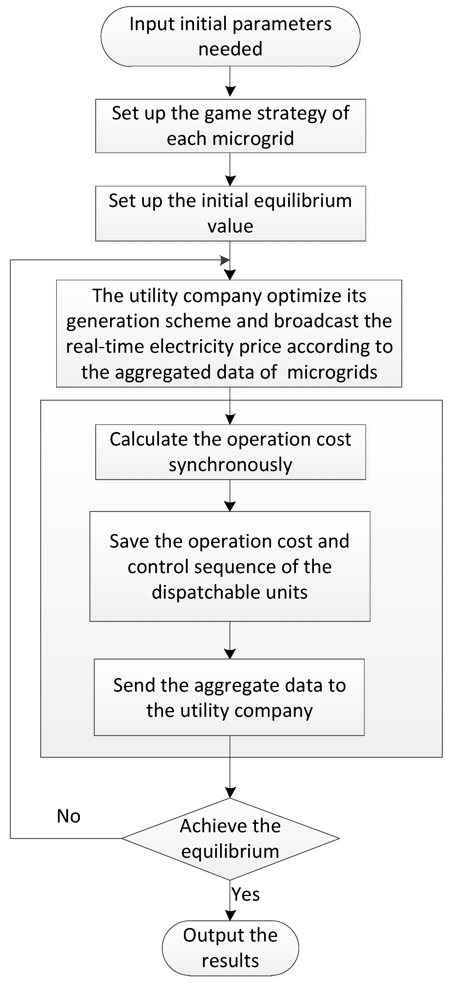
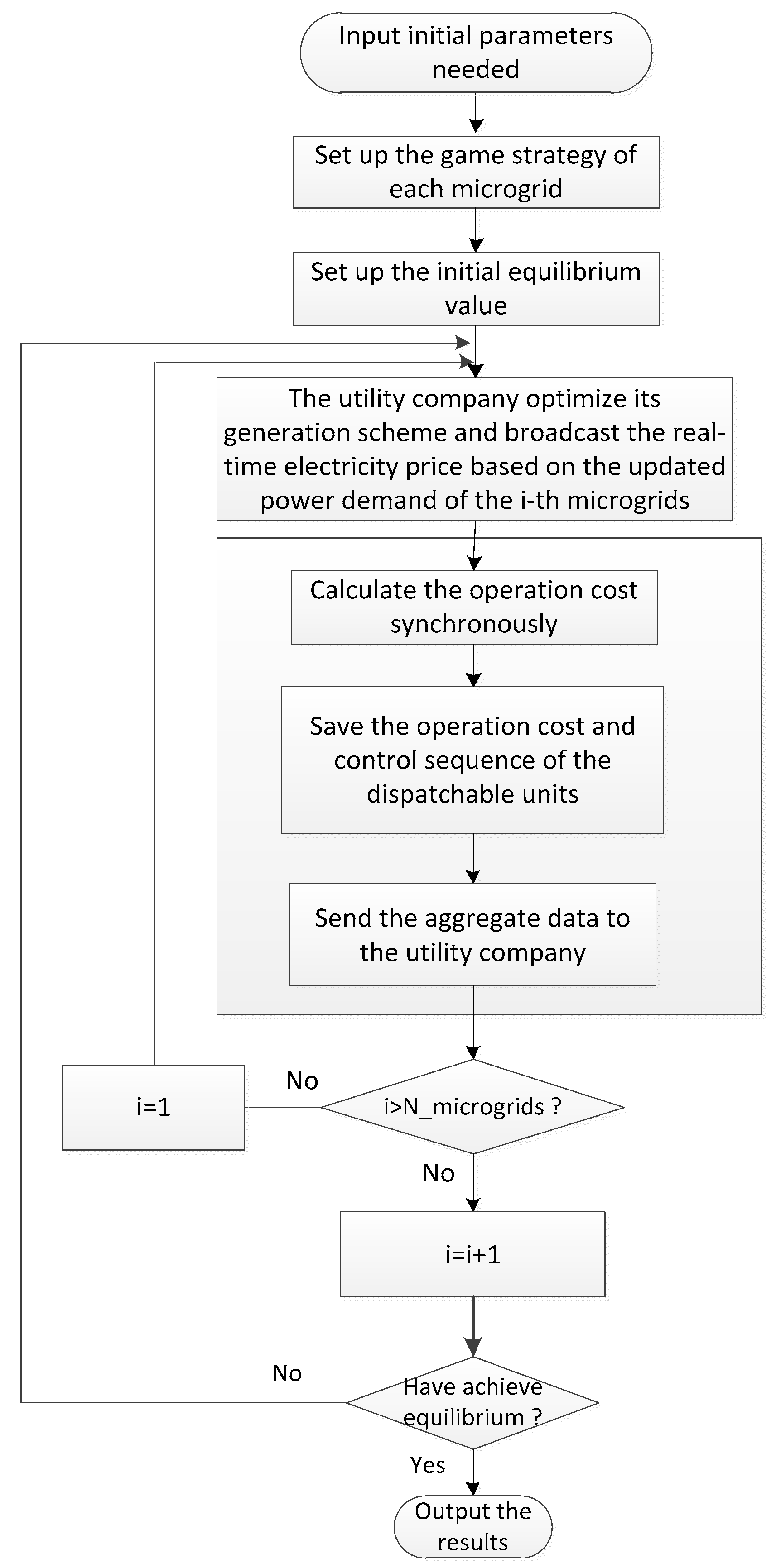
3. The Demand Response Algorithm

In most of studies, a sequential-like optimization algorithm is often used to solve the demand response problem. However, the algorithm has a guaranteed convergence: it only suits a small power system. Therefore, in this study, a parallel distributed demand response algorithm is proposed. The optimal demand response operation of each microgrid is implemented synchronously. This algorithm allows the EMS of the microgrid to autonomously minimize their own operation cost by properly scheduling the dispatchable units, e.g., ESD units, CDG units, curtailable loads, and schedulable loads. A non-cooperative games model is used to describe the relationship among the microgrids. Moreover, for guaranteeing the convergence of the proposed algorithm, a penalty function is introduced as that is used in [14].

The penalty cost in iteration $k$ ($k\ge 2$) is calculated as follows,

$$C_{i,penalty}^k={\lambda }_i^k({\Vert (P_{i,Ed}^k-P_{i,Ec}^k)-(P_{i,Ed}^{k-1}-P_{i,Ec}^{k-1})\Vert }_2^2+{\Vert l_{i,load}^k-l_{i,load}^{k-1}\Vert }_2^2+{\Vert P_{i,CDG}^k-P_{i,CDG}^{k-1}\Vert }_2^2)$$

(26)

where ${\lambda }_i^k$ is a parameter that has close relation to the importance of the $i\mathrm{th}$ microgrid in the power system, and it is used to adjust the iteration steps needed to achieve the convergence. $P_{i,Ed}^k$ is a vector that denotes the discharging power of the ESD units in microgrid $i$ during the future control horizon. The other variables can be thought of with the same principle.

The formulation of ${\lambda }_i^k$ is shown as follow,

$${\lambda }_i^k\propto {\left({\Vert \frac{{\sum }_{t=1}^T{P}_{utility}^k\left(t\right)}{{\sum }_{t=1}^T\left(P_{i,gridI}^k\left(t\right)+P_{i,gridO}^k\left(t\right)\right)}\Vert }_2^2\right)}^{\alpha }$$

(27)

where $\alpha >0$ is the adjustment coefficient, and its value is determined by the specially power grid condition. Equation (27) shows that the less power exchanged between the microgrid and the utility company, the less important is the demand response, and the higher ${\lambda }_i^k$ will be obtained. In the contrast, the more power exchanged between the microgrid and the utility company, the more important is the demand response, and the lower ${\lambda }_i^k$ value that will be obtained. It can effectively avoid a large fluctuant for the little important microgrid in successive iteration steps.

Therefore, the objective function used for the microgrids in the $k\mathrm{th}$ ($k>1$) is,

$$C_i+C_{i,penalty}^k$$

(28)

when the algorithm converges, $C_{i,penalty}^k\approx 0$. On the other side, when $k=1$ the objective function for the microgrids is $C_i$.

The criterion used to check the convergence of the distributed demand response strategy is shown as follows,

$$\begin{array}{c}\Vert C^k\left(P_{utility}\right)-C^{k-1}\left(P_{utility}\right)\Vert \le {\xi }_1\\ \left|\Vert (P_{i,gridI}^k-P_{i,gridO}^k)\Vert -\Vert P_{i,gridI}^{k-1}-P_{i,gridO}^{k-1}\Vert \right|\le {\xi }_2\\ \Vert l_{i,load}^k-l_{i,load}^{k-1}\Vert \le {\xi }_3\\ \Vert P_{i,CDG}^k-P_{i,CDG}^{k-1}\Vert \le {\xi }_4\end{array}$$

(29)

where ${\xi }_1$, ${\xi }_2$, ${\xi }_3$, ${\xi }_4$ are the corresponding parameters to evaluate the equilibrium; their values are determined by the specially system condition.

Therefore, the procedure of the distributed demand response algorithm is shown in Figure 2.

4. Simulation and Results

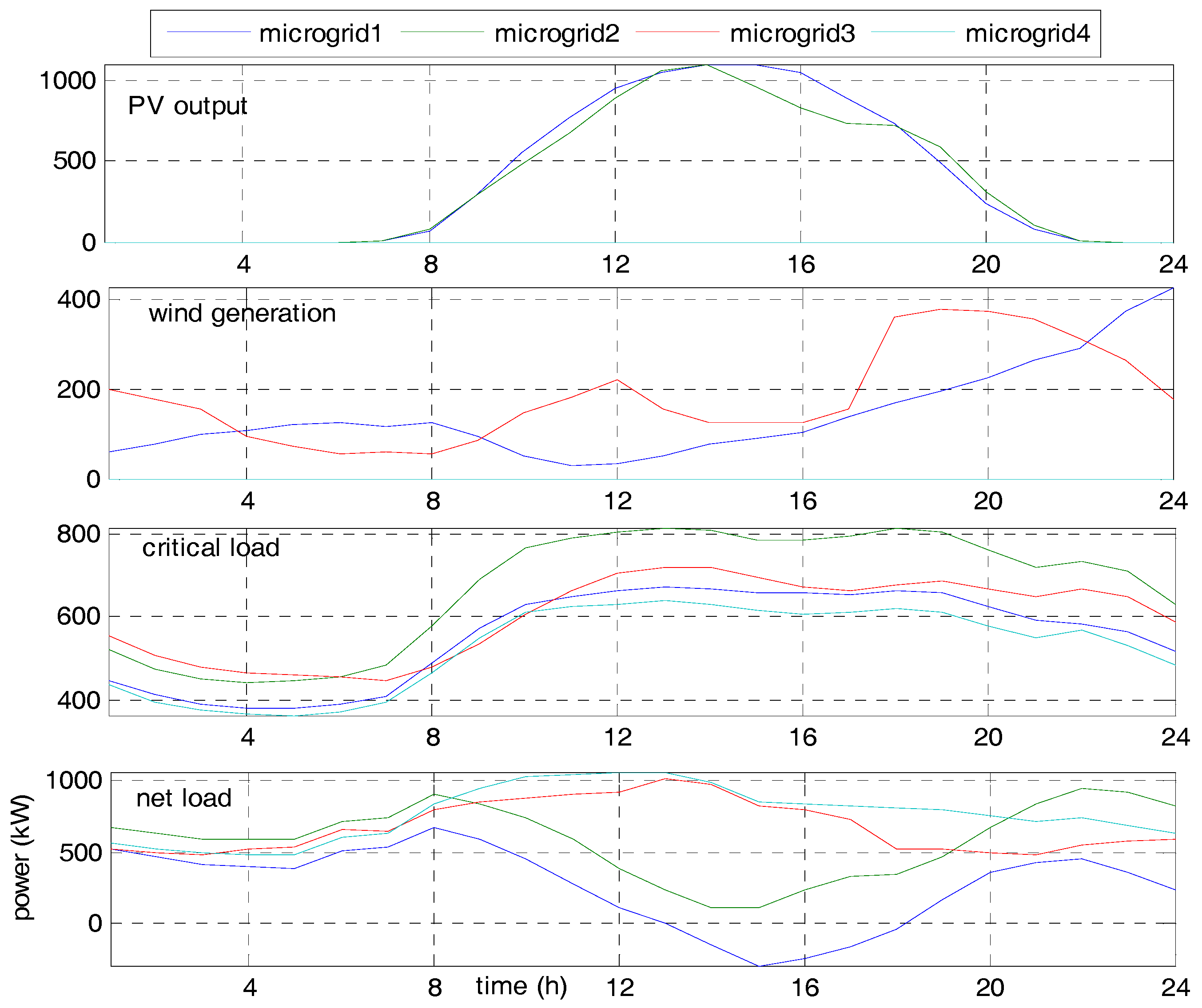
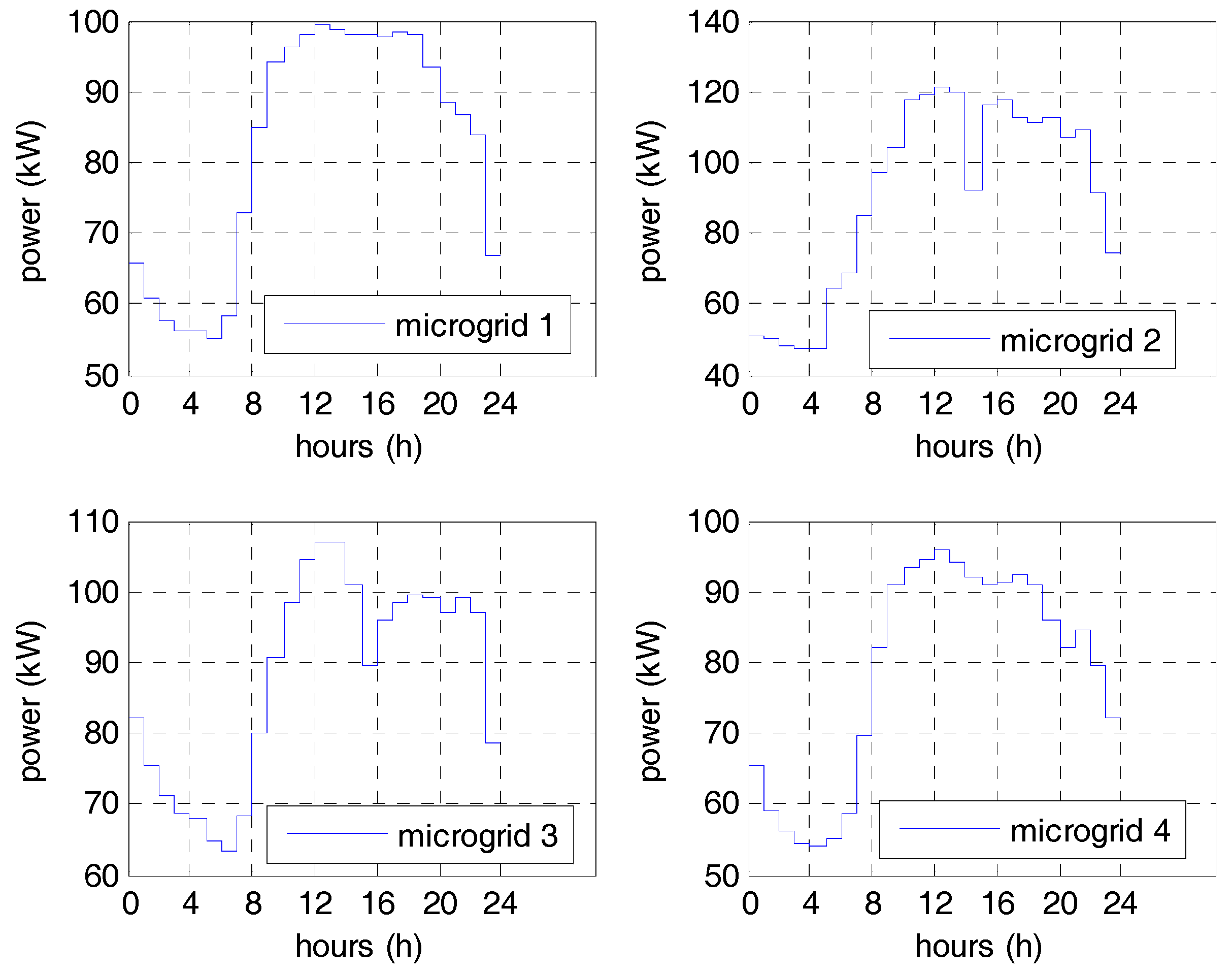
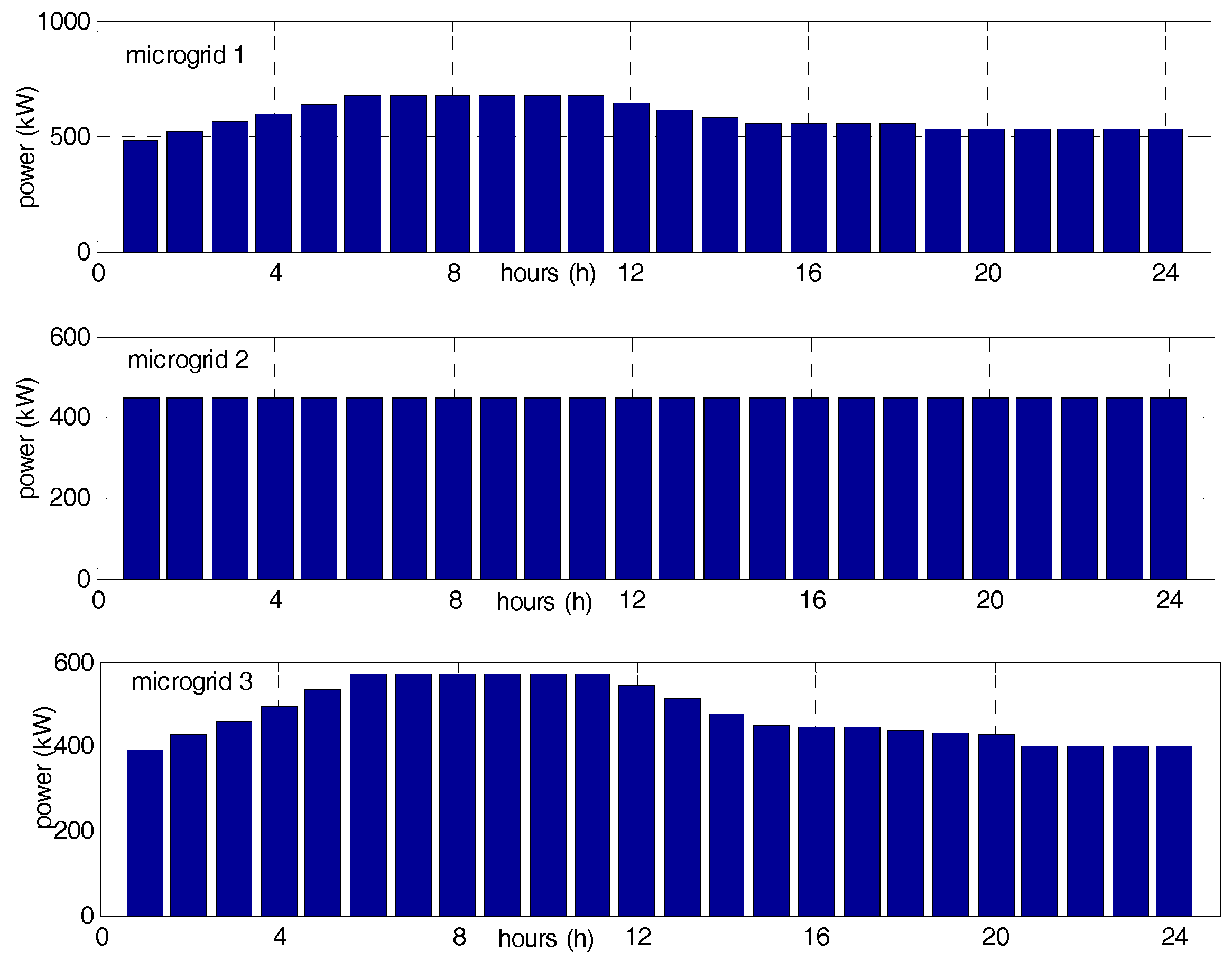
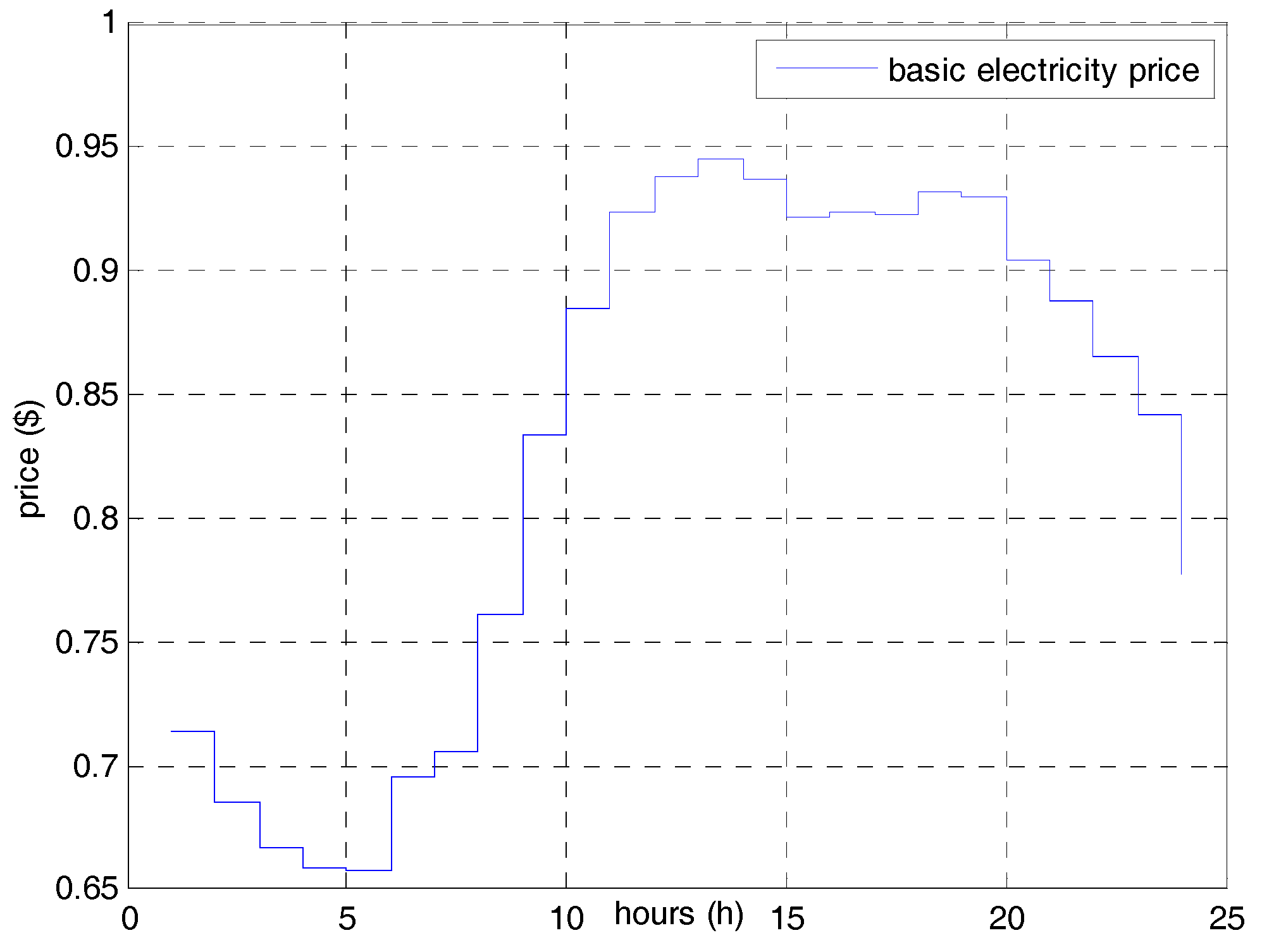
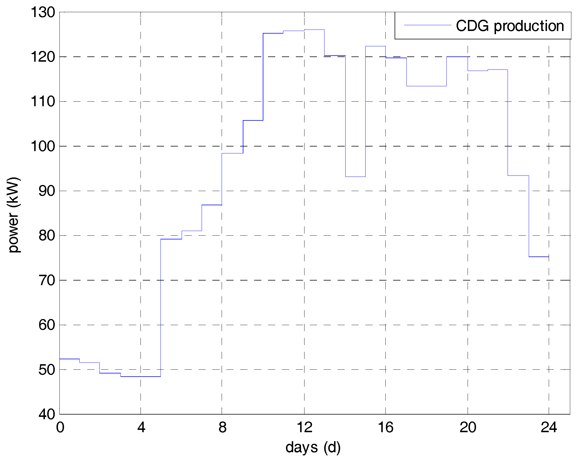
4.1. Test Description

In order to verify the proposed distributed optimal demand response strategy, a power system similar to Figure 1 is used. Four microgrid users, a utility company is integrated into this power system; the microgrids user is scheduled and controlled by its own EMS, and the generators of the utility company are controlled by the utility company controller. As mentioned earlier, not all microgrids have all the dispatchable units discussed in the above, most of them only have parts of the units.

History data used in this study is collected and modified from [28], Belgium’s electricity transmission system operator. The primary and forecasted data of wind generation, PV power production, critical load demand, and the net-load demand at the beginning of a day is shown in Figure 3. The control and prediction horizon $T$ is one day and the time interval $∆t$ between two-time steps is one hour. The capacity of the PV plants and wind farms, the maximum of the critical load demand, and the maximum purchasing/selling power of each microgrid is listed in

Table 1. Limits of the photovoltaic (PV), wind, purchasing/selling power, and the critical loads.

	PV Capacity (kW)	Wind Capacity (kW)	Maximum Exchanging Power (kW)	Maximum Critical Load (kW)
Microgrid 1	1100	530	1000	670
Microgrid 2	100	0	1000	810
Microgrid 3	0	660	1200	720
Microgrid 4	0	0	1500	640

. We assume that the curtailable load demand in each time interval is 30% of that of the critical load demand. The generators of the utility company can fully satisfy the demand of the microgrids, and we use the parameter of a generator to represent the whole parameter of the generator units. Thus, the parameter of the utility company is listed in

Table 2. Power limits of the controllable generators.

	Max Power	Min Power	Ramp Rate	Cost Coefficients
Microgrid 2	450	25	400	0.0055/0.44
Utility company	4000	100	4000	0.00018/0.30

, and the parameter of the CDG unit is also listed in Table 2. The parameter of ESD units used in this the average power generation is 3.3712 × 10³ kW paper is listed in

Table 3. Parameters of the ESD (energy storage devices) units.

	Max Charge/Discharge Power	Min Charge/Discharge Power	O&M Cost	Min Energy Level	Max Energy Level	Charge/Discharge Efficiency
Microgrid 1	320	10	0.054	128	960	0.95
Microgrid 2	280	16	0.058	120	900	0.95
Microgrid 3	240	12	0.057	104	780	0.95

; the initial state of the ESD units at the beginning of one day must near the middle energy level to respond to the emergency conditions.

According to the rate-of-return regulations, we assume the actual purchasing electricity price is 1.2 times of the basic price, which is calculated by Equation (5). The maximum curtailment of the curtailable loads in each time interval is 0.5, but the penalty coefficient to the curtailment action is 3 times the basic electricity price in that time interval, because the curtailment operation of the loads only can be used in emergency conditions.

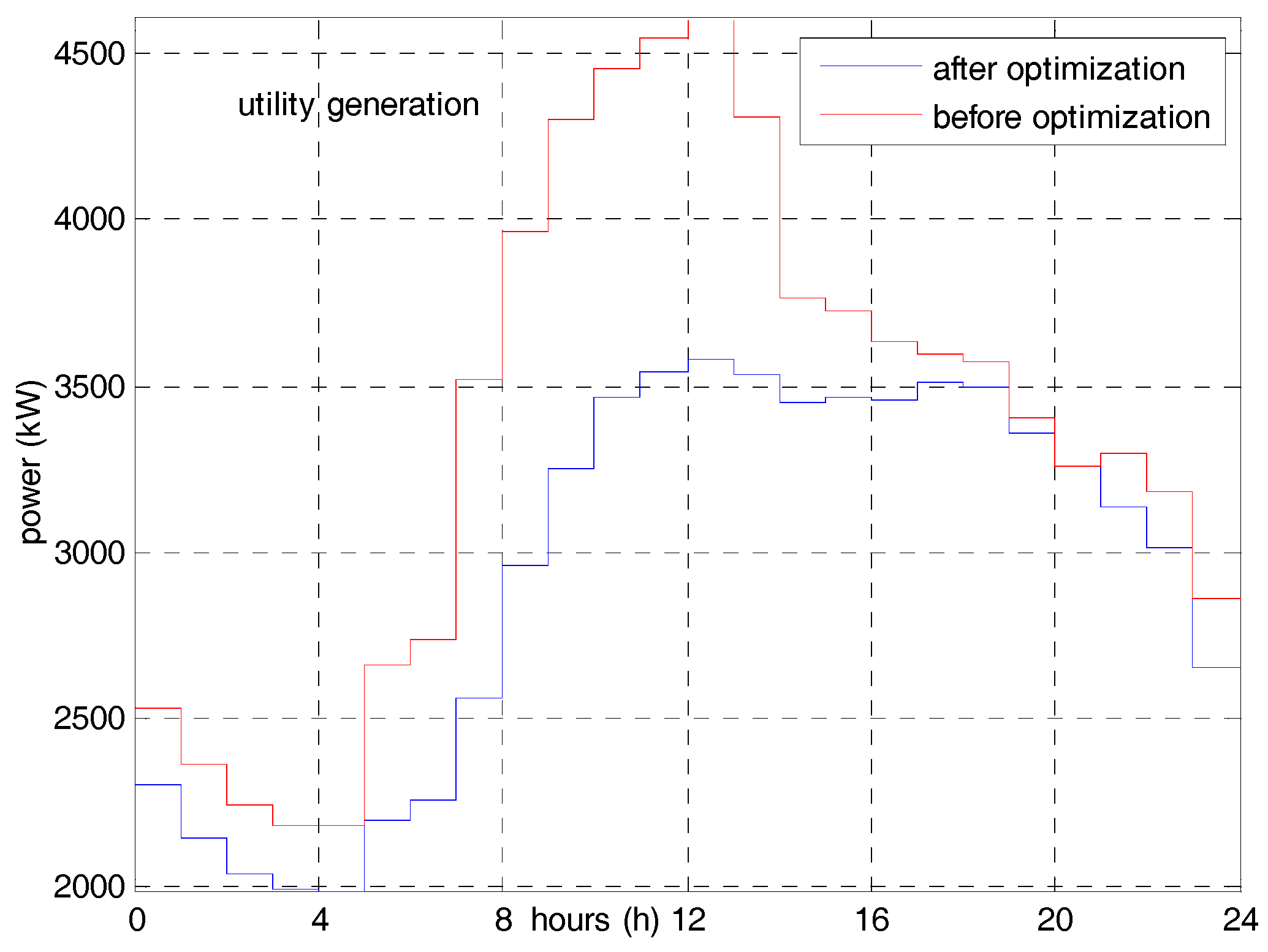
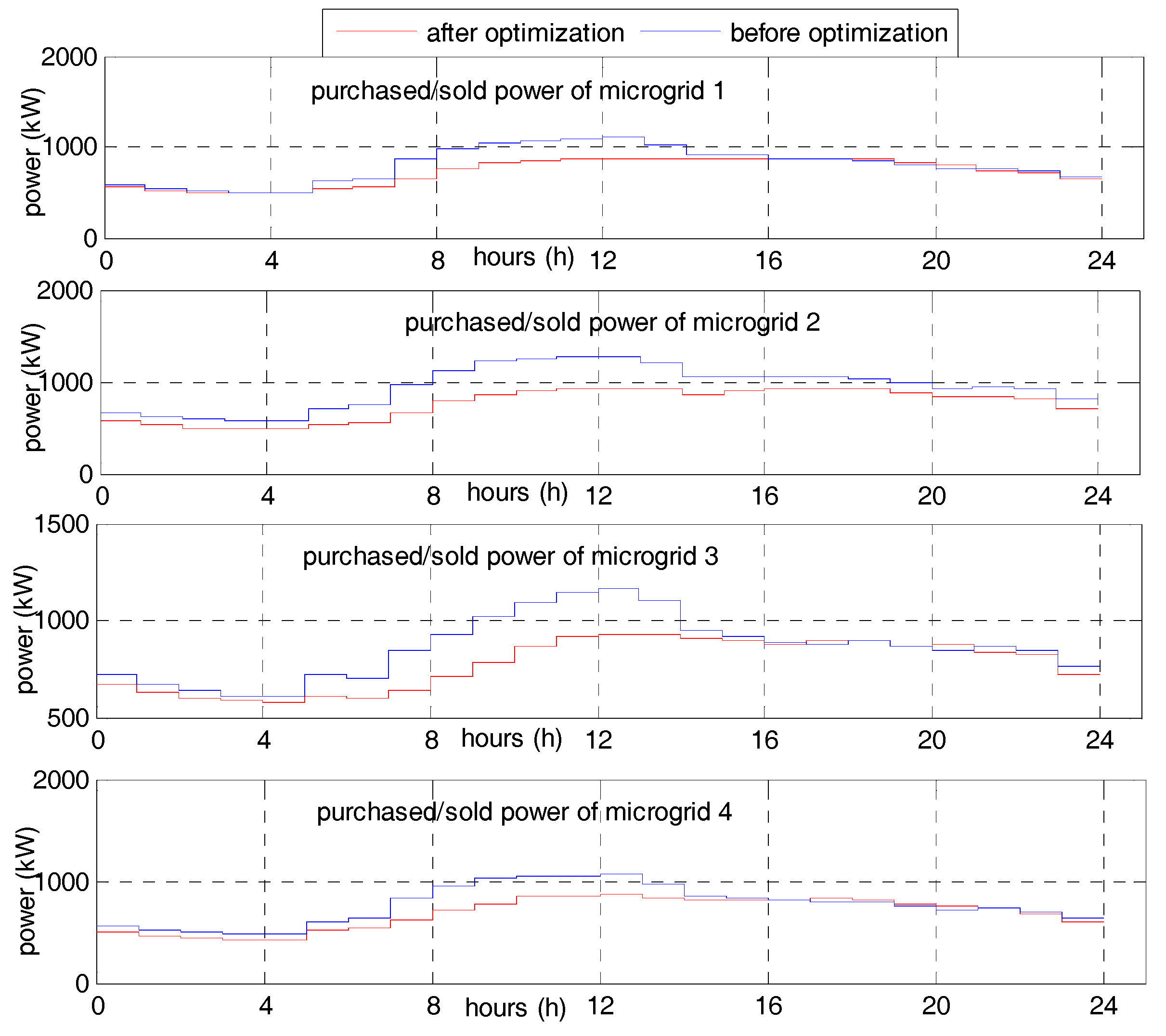
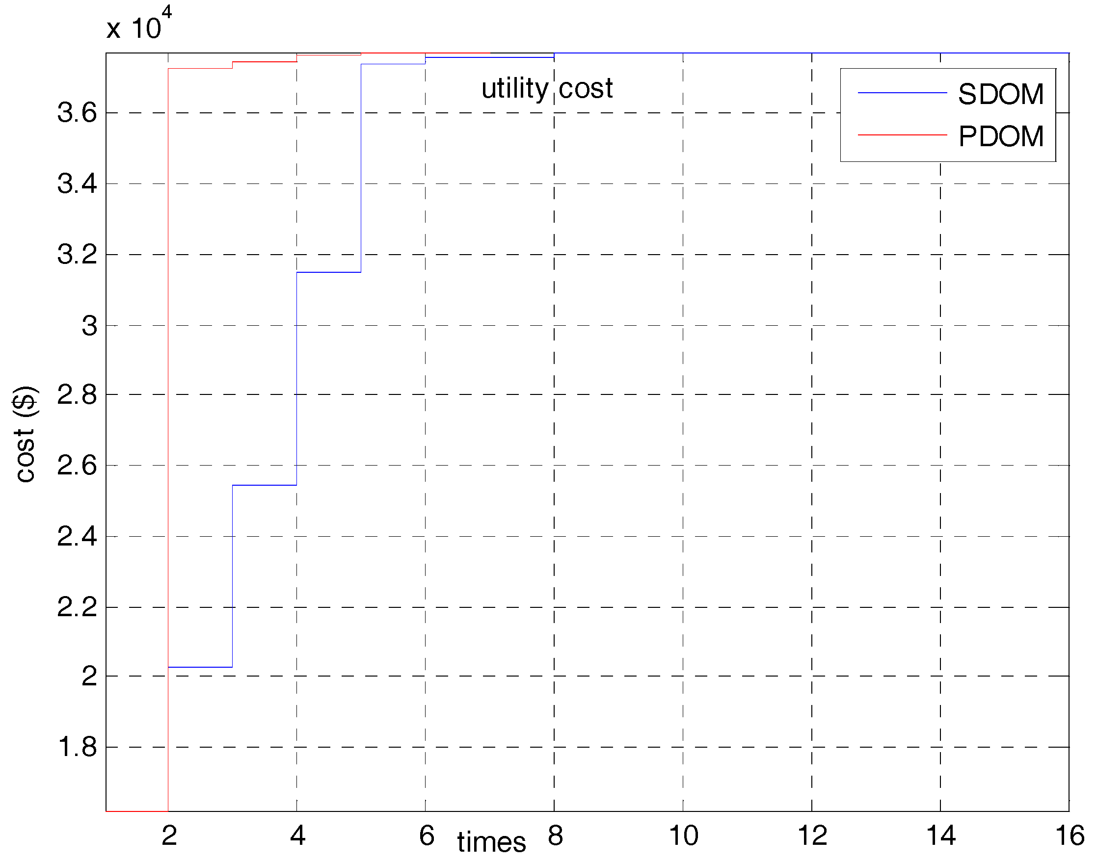
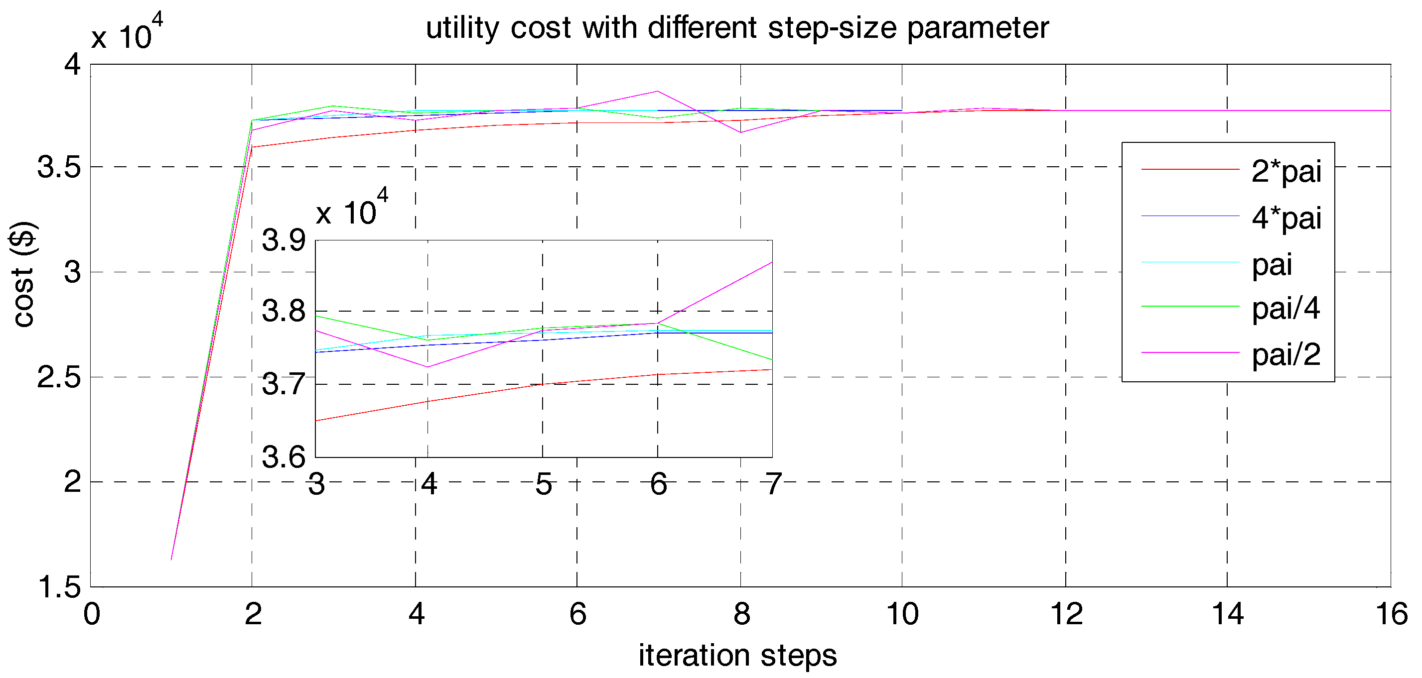
4.2. Simulation Results

All simulations were run on the PC with Intel(R) Core(TM) i5-3470 CPU @3.2 GHz and 8.00 GB memory. The ILOG’s CPLEX v.12 optimization solver is utilized for solving the mixed integer linear programming (MILP) model; MATLAB 2013a and YALMIP toolbox are used for linking the CPLEX solver and computing the model.

Figure 4 shows the generation of the utility company before and after optimization. Seen from the blue line, the maximum generation power is 4.6028 × 10³ kW, the average power generation is 3.3712 × 10³ kW, but the minimum generation power is only 2.1804 × 10³ kW; thus, the peak-to-valley ratio and peak-to-average ratio are 2.111 and 1.3653, respectively. Meanwhile, for the red line, the maximum generation is 3.5836 × 10³ kW, the average power generation is 2.9438 × 10³ kW, but the minimum generation power is only 1.9873 × 10³ kW; thus, the peak-to-valley ratio and peak-to-average ratio are 1.803 and 1.2173. Therefore, Figure 5 shows that the proposed algorithm can effectively reduce the peak load of smart grid, increase the peak-to-valley ratio and peak-to-average ratio, and decrease the operation cost of the utility company.

Figure 5 further indicates the advantage of our proposed algorithm. The peak load of microgrids is reduced effectively. The peak load of each microgrid decreases by 232.6624 kW, 355.0183 kW, 237.9369 kW, and 192.9663 kW, respectively. Though each microgrid curtails part of flexible loads at the same time, as shown in Figure 6, the curtailed flexible load, however, is obviously lower than the decreased power.

Figure 7 shows energy variation of the BESS in each microgrid. Since the electricity price is determined by the coordination of all microgrids, all BESS units take part in the coordination. This results in the fact that the BESS units are not as important as in traditional power systems. The BESS of microgrid 1 and microgrid 3 both charge power when the electricity price is low and discharge power when electricity price is high, see Figure 8. For the same reason, the CDG unit, as shown in Figure 9, generates more power during high electricity price periods than low electricity price periods.

5. Discussion

In order to analyze the superiority of the parallel distributed optimization method (PDOM) proposed in this paper, a sequential distributed optimization method (SDOM) is utilized as the base method. The schematic diagram of the SDOM is shown as follows:

As shown in Figure 10, the utility company has to keep calculating its generation schedule and real-time electricity price once a microgrid updates its own purchasing/selling schedule or the operation schedules of the dispatchable units in it.

Table 4. Operation costs of each microgrid for the two distributed optimization methods.

	Cost of SDOM	Cost of PDOM
Microgrid 1	5291 $	5266 $
Microgrid 2	11,303 $	11,349 $
Microgrid 3	13,598 $	13,574 $
Microgrid 4	15,314 $	15,342 $

indicates the operation cost of microgrids for PDOM and SDOM. From the table, we can see that the total operation cost induced by PDOM and SDOM is nearly the same. The PDOM is only 25 $ more than SDOM. However, it can be seen from Figure 11 that the utility only needs to update its generation schedule seven times for the PDOM so as to achieve equilibrium; the value for the SDOM is sixteen times. Moreover, the utility cost for the PDOM when it achieves the equilibrium is 37,738.9 $, and the utility cost for the SDOM is 37,721.7 $.

Next, we discuss the impacts of step-size parameter to the PDOM convergence. We select the base $\pi =1$ as used in Equation (27) and then perform a series of simulations with the parameter ${\pi }_{sim}$ selected as $1/4\pi$, $1/2\pi$, $\pi$, $2\pi ,$ and $4\pi$. Experimental results are shown in Figure 12.

The results in Figure 12 indicates that the convergence of the game theory among microgrids can be achieved as few as seven iterations when ${\pi }_{sim}=1$, ten iteration steps when ${\pi }_{sim}=1/2\pi$, and fifteen iteration when ${\pi }_{sim}=1/4\pi$. The lower the ${\pi }_{sim}$, the more iterations the PDOM needs to converge. This is because the constraint exerted on the microgrid is not enough to prevent large power change. Meanwhile, the larger the ${\pi }_{sim}$, the more iterations of the PDOM need to converge. Specifically, nine iterations are needed to converge when ${\pi }_{sim}=2\pi$, and sixteen iterations when ${\pi }_{sim}=4\pi$. The reason is that a large parameter will strictly constrain the power change in the consecutive iteration steps, such that the convergence speed is slowed down. Such results confirm again the conclusions of [13,17].

6. Conclusions and Future Studies

This study proposed a distributed optimal demand response approach to minimize the operation cost of multi-microgrids in a smart grid. The power purchasing/selling of the microgrid and the operation routines of the dispatchable units are controlled by EMS of each individual microgrid. A mixed integer quadratic programming model is formulated to describe the energy management problem. Experimental results show that the proposed method is both effective and efficient.

With respect to future studies, the first thing is to further investigate the cooperative games among multiple microgrids. Second, the model is solved using CPLEX; however, the CPLEX might not be effective when the problem scale becomes large. Therefore, we would like also to develop new effective solvers, e.g., evolutionary algorithms. Moreover, this study has only considered minimizing the operation cost. In fact, there are other objectives, e.g., related to environment, that need to be optimized. Thus, a multi-objective optimization model and algorithms [29,30,31,32,33] should also be considered.

References

1. Wang, W.; Xu, Y.; Khanna, M. A survey on the communication architectures in smart grid. Comput. Netw. 2011, 55, 3604–3629. [Google Scholar] [CrossRef]
2. Barroso, L.A.; Rudnick, H.; Sensfuss, F.; Linares, P. The Green Effect. IEEE Power Energy Mag. 2010, 8, 22–35. [Google Scholar] [CrossRef]
3. Yassine, A. Cooperative Games among Consumers in the Smart Grid. In Proceedings of the 2013 IEEE GCC Conference and Exhibition, Doha, Qatar, 17–20 November 2013; pp. 70–75. [Google Scholar]
4. Zhang, D.; Shah, N.; Papageorgiou, L.G. Efficient energy consumption and operation management in a smart building with microgrid. Energy Convers. Manag. 2013, 74, 209–222. [Google Scholar] [CrossRef]
5. Parisio, A.; Glielmo, L. A Mixed Integer Linear Formulation for Microgrid Economic Scheduling. In Proceedings of the Virtual Power Plants, Distributed Generation, Microgrids, Renewables and Storage (IEEE SmartGridComm), Brussels, Belgium, 17–20 October 2011; pp. 505–510. [Google Scholar]
6. Zhang, Y.; Zhang, T.; Liu, Y.; Guo, B. Stochastic Model Predictive Control for Energy Management Optimization of an Energy Local Network. Proc. CSEE 2016, 36, 3451–3462. [Google Scholar]
7. Palensky, P.; Dietrich, D. Demand Side Management: Demand Response, Intelligent Energy Systems, and Smart Loads. IEEE Trans. Ind. Inform. 2011, 7, 381–388. [Google Scholar] [CrossRef]
8. Yang, P.; Chavali, P.; Nehorai, A. Parallel Autonomous Optimization of Demand Response with Renewable Distributed Generators. In Proceedings of the IEEE SmartGridComm 2012 Symposium-Demand Side Management, Demand Response, Dynamic Pricing, Tainan, Taiwan, 5–8 November 2012; pp. 55–60. [Google Scholar]
9. Wu, Q.; Wang, L.; Cheng, H. Research of TOU power price based on multi-objective optimization of DSM and costs of power consumers. In Proceedings of the International Conference on Electric Utility Deregulation, Restructuring and Power Technologies, Hong Kong, China, 5–8 April 2004; pp. 343–348. [Google Scholar]
10. Celebi, E.; Fuller, J.D. A model for efficient consumer pricing schemes in electricity markets. IEEE Trans. Power Syst. 2007, 22, 60–67. [Google Scholar] [CrossRef]
11. Chen, C.; Wang, J. MPC-Based Appliance Scheduling for Residential Building Energy Management Controller. IEEE Trans. Smart Grid 2013, 4, 1401–1410. [Google Scholar] [CrossRef]
12. Dominguez-Garcia, A.D.; Hadjicostis, C.N. Distributed Algorithms for Control of Demand Response and Distributed Energy Resources. In Proceedings of the 2011 50th IEEE Conference on Decision and Control and European Control Conference (CDC-ECC), Orlando, FL, USA, 12–15 December 2011; pp. 27–32. [Google Scholar]
13. Yang, P.; Chavali, P.; Gilboa, E.; Nehorai, A. Parallel Load Schedule Optimization with Renewable Distributed Generators in Smart Grids. IEEE Trans. Smart Grid 2013, 4, 1431–1441. [Google Scholar] [CrossRef]
14. Tan, Z.; Yang, P.; Nehorai, A. An Optimal and Distributed Demand Response Strategy with Electric Vehicles in the Smart Grid. IEEE Trans. Smart Grid 2014, 5, 861–869. [Google Scholar] [CrossRef]
15. Mírez, J.; Hernández-Callejo, L.; Horn, M.; Bonilla, L.M. Simulation of DC Microgrid and Study of Power and Battery Charge/Discharge Management. Energetic Technol. Energ. Energy Distrib. 2017, 92, 673–679. [Google Scholar]
16. Mírez, J. A modeling and simulation of optimized interconnection between DC microgrids with novel strategies of voltage, power and control. In Proceedings of the 2017 IEEE Second International Conference on DC Microgrids (ICDCM), Núremberg, Germany, 27–29 June 2017; pp. 536–541. [Google Scholar]
17. Ou, T.C.; Hong, C.M. Dynamic operation and control of microgrid hybrid power systems. Energy 2014, 66, 314–323. [Google Scholar] [CrossRef]
18. Ou, T.C.; Su, W.-F.; Liu, X.-Z.; Huang, S.-J.; Tai, T.-Y. A Modified Bird-Mating Optimization with Hill-Climbing for Connection Decisions of Transformers. Energies 2016, 9, 671. [Google Scholar] [CrossRef]
19. Ou, T.C.; Lu, K.H.; Huang, C.J. Improvement of Transient Stability in a Hybrid Power Multi-System Using a Designed NIDC (Novel Intelligent Damping Controller). Energies 2017, 10, 488. [Google Scholar] [CrossRef]
20. Amini, M.H.; Nabi, B.; Haghifam, M.R. Load management using multi-agent systems in smart distribution network. In Proceedings of the 2013 IEEE Power and Energy Society General Meeting, Vancouver, BC, Canada, 21–25 July 2013; pp. 1–5. [Google Scholar]
21. Bui, V.H.; Hussain, A.; Kim, H.M. Optimal Operation of Microgrids Considering Auto-Configuration Function Using Multiagent System. Energies 2017, 10, 1484. [Google Scholar] [CrossRef]
22. Gomez-Sanz, J.J.; Garcia-Rodriguez, S.; Cuartero-Soler, N.; Hernandez-Callejo, L. Reviewing Microgrids from a Multi-Agent Systems Perspective. Energies 2014, 7, 3355–3382. [Google Scholar] [CrossRef]
23. Haider, H.T.; See, O.H.; Elmenreich, W. Residential demand response scheme based on adaptive consumption level pricing. Energy 2016, 113, 301–308. [Google Scholar] [CrossRef]
24. Safamehr, H.; Rahimi-Kian, A. A cost-efficient and reliable energy management of a micro-grid using intelligent demand-response program. Energy 2015, 91, 283–293. [Google Scholar] [CrossRef]
25. Ou, T.C. A novel unsymmetrical faults analysis for microgrid distribution systems. Int. J. Electr. Power Energy Syst. 2012, 43, 1017–1024. [Google Scholar] [CrossRef]
26. Ou, T.C. Ground fault current analysis with a direct building algorithm for microgrid distribution. Int. J. Electr. Power Energy Syst. 2013, 53, 867–875. [Google Scholar] [CrossRef]
27. Erdinc, O. Economic impacts of small-scale own generating and storage units, and electric vehicles under different demand response strategies for smart households. Appl. Energy 2014, 126, 142–150. [Google Scholar] [CrossRef]
28. Grid Data. Available online: http://www.elia.be/en/grid-data/ (accessed on 1 December 2017).
29. Zhang, Y.; Zhang, T.; Wang, R.; Liu, Y.; Guo, B. A Model Predictive Control Based Distributed Coordination of Multi-microgrids in Energy Internet. Acta Autom. Sin. 2017, 43, 1443–1456. [Google Scholar]
30. Wang, R.; Purshouse, R.C.; Fleming, P.J. Preference-inspired co-evolutionary algorithms for many objective optimization. IEEE Trans. Evol. Comput. 2013, 17, 474–494. [Google Scholar] [CrossRef]
31. Wang, R.; Zhang, Q.F.; Zhang, T. Decomposition based algorithms using Pareto adaptive scalarizing methods. IEEE Trans. Evol. Comput. 2016, 20, 821–837. [Google Scholar] [CrossRef]
32. Wang, R.; Li, G.; Ming, M.; Wu, G.; Wang, L. An efficient multi-objective model and algorithm for sizing a stand-alone hybrid renewable energy system. Energy 2017, 141, 2288–2299. [Google Scholar] [CrossRef]
33. Ming, M.; Wang, R.; Zha, Y.B.; Zhang, T. Multi-objective Optimization of Hybrid Renewable Energy System using an Enhanced Evolutionary Multi-objective Algorithm. Energies 2017, 10, 674. [Google Scholar] [CrossRef]
Figure 1. Schematic diagram of the smart grid with multiple microgrids.
Energies 11 00215 g001
Figure 2. Schematic diagram of the smart grid calculated by parallel distributed method.
Energies 11 00215 g002
Figure 3. Schematic of the history data used in present paper.
Energies 11 00215 g003
Figure 4. The utility generation before and after optimization.
Energies 11 00215 g004
Figure 5. The purchased/sold power of all the microgrids before and after optimization.
Energies 11 00215 g005
Figure 6. The curtailed flexible loads for microgrids 1 to 4.
Energies 11 00215 g006
Figure 7. Varying of BESS (battery energy storage system) energy level for all the microgrids.
Energies 11 00215 g007
Figure 8. Basic electricity price of the smart grid.
Energies 11 00215 g008
Figure 9. The generation of CDG (controllable distributed generation) unit in microgrid 2.
Energies 11 00215 g009
Figure 10. Schematic diagram of the smart grid calculated by sequential distributed method.
Energies 11 00215 g010
Figure 11. Utility cost at each iteration for PDOM (parallel distributed optimization method) and SDOM (sequential distributed optimization method).
Energies 11 00215 g011
Figure 12. Convergence of PDOM with different step-size parameters.
Energies 11 00215 g012