Collaborative Scheduling between OSPPs and Gasholders in Steel Mill under Time-of-Use Power Price

Abstract

Byproduct gases generated during steel production process are the main fuels for on-site power plants (OSPPs) in steel enterprises. Recently, with the implementation of time-of-use (TOU) power price in China, increasing attention has been paid to the collaborative scheduling between OSPPs and gasholders. However, the load shifting potential of OSPPs has seldom been discussed in previous studies. In this paper, a mixed integer linear programming (MILP)-based scheduling model is built to evaluate the load shifting potential and the corresponding economic benefits. A case study is conducted on two steel enterprises with different configurations of OSPPs, and the optimal operation strategy is also discussed.

1. Introduction

As one of the most energy intensive industries, the steel-making industry accounts for approximately 15% of the total electricity consumption in China [1]. To decrease the power purchase as well as increase the reliability of power supply, plenty of on-site power plants (OSPP) are built in steel enterprises. Generally, these OSPPs can cover 40–80% of overall electricity consumption in steel enterprises, and the remaining demand is supplied by the main grid [2,3].

Byproduct gases generated from the steel production process are the main fuels for OSPPs. Because the steel production process is unstable, both the production and consumption of byproduct gases suffer from fluctuations. Currently, steel enterprises establish buffer units such as gasholders and boilers to reduce the fluctuations, and thus decrease levels of byproduct gas flaring or shortage [4]. Plenty of studies have been conducted on the optimal scheduling of byproduct gases in the steel sector, where linear programming (LP), mixed integer linear programming (MILP), genetic algorithms (GA) and other optimization methods have already been successfully applied [5,6].

Recently, with the implementation of time-of-use (TOU) power price in China, increasing attention has been paid to the collaborative scheduling between OSPPs and gasholders. Through reducing the electricity generation during the valley price period (VPP) and increasing the electricity generation during the peak price period (PPP), the peak-valley shifting of the electricity generation can be achieved and the electricity purchasing cost can be reduced.

However, few studies have been conducted on this topic. He and Wang proposed a static model to evaluate the economic benefits of peak load shifting of OSPPs in the Chinese steel industry under TOU power price [7]. Zeng considered the power exchange cost with the main grid and proposed a mixed integer linear programming (MILP)-based scheduling model for a byproduct gas system. The results demonstrated that the overall operation cost could be reduced by 6% [8]. We considered the influence of the operation load on boiler efficiency and applied Pareto optimality and fuzzy sets to determine the best compromise solution for byproduct gas scheduling under TOU power price [3].

The abovementioned models usually generate a compromised solution between the stability and the profitability of the byproduct gas system, and the maximum load shifting potential of this method is still unclear. Therefore, an improved MILP model is proposed in this paper. To our knowledge, this is the first work to consider the configuration difference of OSPPs in the collaborative scheduling under the TOU tariff. Of special emphasis is the evaluation of load shifting potential for different configurations of OSPPs. In addition, the optimal operation strategy under the TOU tariff is also discussed.

2. Problem Statements

A typical byproduct gas system is outlined in Figure 1a. Around 60% of the byproduct gases were used for heating in the metallurgical process, and the flexibility of the gas consumption is very limited because the regular steel production is stable [9]. On the other hand, the rest of the byproduct gases can be adjusted more flexibly, either consumed by the OSPPs or stored in gasholders. Generally, the OSPPs in steel plants include two types of generation units: combined cycle power plants (CCPPs) and simple steam boilers as well as their corresponding turbines, as shown in Figure 1a.

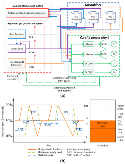
Figure 1. (a) Diagram of a byproduct gas system in a steel plant; (b) schematic view of the collaboration between the gasholder level and the electricity generation of the on-site power plant (OSPP) under the time-of-use (TOU) tariff.

The imbalance between the production and consumption of byproduct gases makes the overall system suffer from fluctuations, which is liable to make gas flaring necessary or negatively affect the gas supply of the boilers and CCPPs. Therefore, in previous studies, gasholder levels were preferably sustained around the middle level, since the middle level possesses the best anti-fluctuation ability [3,4,9,10,11]. The significance of the gas storage function of the gasholder becomes obvious for the electricity cost reduction if the time-of-use (TOU) electricity tariff is considered [12,13,14]. Generally, the electricity price during the peak period is two to three times higher than that in the valley period in China [15,16]. This offers the possibility of reducing the electricity cost by producing more electricity in the OSPP during the PPP and purchasing more electricity from the main grid during the VPP, with the gas storage level in the gasholder changing between the higher and lower levels, as shown in Figure 1b.

In order to access the maximum load shifting potential of the byproduct gas system, the gasholders are required to fully utilize their storage ability [5,17], and the safety of the gasholders is ensured by constraints defined in Section 3.2.3 [18,19].

3. Mathematical Model

3.1. Objective Function

The objective function of the proposed model is to minimize the electricity purchasing cost of the byproduct gas system under the TOU tariff, as shown in Equation (1):

$$Y=\min \{EPC\}=C_t^{\mathrm{elec}}{\displaystyle \sum _{t=1}^P{E}_{t,\mathrm{pur}}}=C_t^{\mathrm{elec}}{\displaystyle \sum _{t=1}^P(E_{t,\mathrm{dem}}-E_{t,\mathrm{gen}})}$$

(1)

where $C_t^{\mathrm{elec}}$, $E_{t,\mathrm{dem}}$, $E_{t,\mathrm{pur}}$, and $E_{t,\mathrm{gen}}$ are the unit price, overall electricity demand, electricity purchased from the main grid, and electricity generated from the OSPP during time period t, respectively; lastly, P stands for scheduling periods. It should be noted that selling power back to the grid is not considered in the proposed model.

3.2. Constraints

3.2.1. Mass Balance

The mass balance of the byproduct gases is shown in Equation (2), where $V_{j,t}$ and $V_{j,t-1}$ are the holder levels of byproduct gas j for period t and period t − 1, respectively; furthermore, B, C, and G represent boilers, CCPPs, and byproduct gases, respectively. The difference between these levels is equal to the surplus volume of the byproduct gases (production minus consumption) in the steel-making process during ∆t, minus the difference of byproduct gas j consumption in the boilers and CCPPs during ∆t. The mass balance of steam is presented in Equation (3), where $F_{i,t}^{\mathrm{stm}}$ is the steam generated from the boilers, which is the sum of the steam consumed in the steel-making process ($F_{i,t}^{\mathrm{dem}}$) and that consumed by the turbines ($F_{i,t}^{\mathrm{tb}}$).

$$V_{j,t}-V_{j,t-1}=(F_{j,t,\mathrm{gen}}-F_{j,t,\mathrm{con}})-{\displaystyle \sum _{i=1}^B{\displaystyle \sum _{j=1}^G(f_{i,j,t}-f_{i,j,t-1})}}\mathsf{\Delta }t-{\displaystyle \sum _{k=1}^C{\displaystyle \sum _{j=1}^G(f_{k,j,t}-f_{k,j,t-1})}}\mathsf{\Delta }t$$

(2)

$$F_{i,t}^{\mathrm{stm}}=F_{i,t}^{\mathrm{dem}}+F_{i,t}^{\mathrm{tb}}$$

(3)

3.2.2. Energy Balance

The energy balance of boiler i and CCPP k is shown in Equations (4) and (5), where $f_{i,t}^{\mathrm{stm}}$, the production of steam (t/h) in boiler i during time period t, is equal to the constant value a_i multiplied by the combustion heat (GJ/h) of the byproduct gases, ${\displaystyle \sum _{j=1}^G{f}_{i,j,t}{H}_j}$ (the sum of the consumption rate (m³/h) of three different gases in boiler i multiplied their corresponding lower heating values, as shown in Equation (4)), plus the constant value b_i,. Furthermore, $p_{k,t}^{}$, the power output (MW) in CCPP k during time period t, is equal to the constant value c_k multiplied by the combustion heat (GJ/h) of the byproduct gases, plus the constant value d_k. a_i, b_i, c_k, and d_k are regression parameters from the historical operation data of boiler i and CCPP k. $f_{i,BFG,t}$, $f_{i,COG,t}$, and $f_{i,LDG,t}$ are the consumption rates of blast furnace gas (BFG), coke oven gas (COG), and Linz-Donawitz process gas (LDG) in boiler i during time period t, respectively. $f_{k,BFG,t}$ and $f_{k,COG,t}$ are the consumption rate of BFG and COG in CCPP k during time period t, respectively. $H_{BFG}$, $H_{COG}$, and $H_{LDG}$ are the lower heating values of BFG, COG, and LDG, respectively. The energy balance of turbine m is shown in Equation (6), where $p{w}_{m,t,\mathrm{gen}}$ is the electricity produced from turbine m, which equals the steam consumption of turbine m multiplied by the enthalpy of steam ($H^{\mathrm{stm}}$) and the steam-electricity converting efficiency (${\eta }_m^{\mathrm{se}}$).

$$f_{i,t}^{stm}=a_i\times {\displaystyle \sum _{j=1}^G{f}_{i,j,t}{H}_j}+b_i=a_i\times (f_{i,BFG,t}{H}_{BFG}+f_{i,COG,t}{H}_{COG}+f_{i,LDG,t}{H}_{LDG})+b_i$$

(4)

$$p_{k,t}^{}=c_k\times {\displaystyle \sum _{j=1}^G{f}_{k,j,t}{H}_j}+d_k=c_k\times (f_{k,BFG,t}{H}_{BFG}+f_{k,COG,t}{H}_{COG})+d_k$$

(5)

$$p{w}_{m,t,\mathrm{gen}}=F_{i,t}^{\mathrm{tb}}{H}_{}^{\mathrm{stm}}{\eta }_m^{\mathrm{se}}$$

(6)

3.2.3. Restrictive Parameters of the Gasholder Operation

The holder level of byproduct gas j must be kept between the lower level (minimum level) and the higher level (maximum level) (Equation (7)). $V_{j,t}$ refers to the holder level of the jth byproduct gas for period t, and $G{H}_{j,\mathrm{HH}}$ and $G{H}_{j,\mathrm{LL}}$ represent the higher and lower levels of gasholder j, respectively. Equation (8) is the storage/supply rate limitation of gasholder j, where $|V_{j,t}-V_{j,t-1}|$ is the holder level change between two adjacent time points (t−1 to t), which should be less than the maximum allowed level ($\mathsf{\Delta }{V}_j^{\max }$).

$$G{H}_{j,\mathrm{HH}}^{}\le V_{j,t}^{}\le G{H}_{j,\mathrm{LL}}^{}$$

(7)

$$\left|V_{j,t}^{}-V_{j,t-1}^{}\right|\le \mathsf{\Delta }{V}_j^{\max }$$

(8)

3.2.4. Restrictive Parameters of the Boiler and CCPP Operation

The operation load and the rate of byproduct gas consumed by the boilers and CCPPs must be kept between the minimum and the maximum levels, as shown by Equations (9) through (12). In these equations, $q_i^{\max }$, $q_k^{\max }$, $q_i^{\min }$, and $q_k^{\min }$ represent the maximum and minimum operation loads of boiler i and CCPP k, respectively, and $f_{i,j}^{\max }$, $f_{k,j}^{\max }$, $f_{i,j}^{\min }$, and $f_{k,j}^{\min }$ represent the maximum and minimum rates of the jth byproduct gas consumed by boiler i and CCPP k, respectively. The change in the jth byproduct gas consumed by boiler i and CCPP k between two adjacent time points should be less than the maximum allowed rate ($\mathsf{\Delta }{f}_{i,j}^{\max }$ and $\mathsf{\Delta }{f}_{k,j}^{\max }$, respectively), as shown in Equations (13) and (14).

$$q_i^{\min }\le {\displaystyle \sum _{j=1}^G{f}_{i,j,t}{H}_j}\le q_i^{\max }$$

(9)

$$q_k^{\min }\le {\displaystyle \sum _{j=1}^G{f}_{k,j,t}{H}_j}\le q_k^{\max }$$

(10)

$$f_{i,j}^{\min }\le f_{i,j,t}^{}\le f_{i,j}^{\max }$$

(11)

$$f_{k,j}^{\min }\le f_{k,j,t}^{}\le f_{k,j}^{\max }$$

(12)

$$\left|f_{i,j,t}-f_{i,j,t-1}\right|\le \mathsf{\Delta }{f}_{i,j}^{\max }$$

(13)

$$\left|f_{k,j,t}-f_{k,j,t-1}\right|\le \mathsf{\Delta }{f}_{k,j}^{\max }$$

(14)

4. Case Study

A case study was conducted for two steel plants in China, namely plant A and plant B. Plant A is a typical middle-sized integrated steel mill with three gasholders and five steam boilers in its byproduct gas system. Plant B is a large-sized integrated steel mill with six gasholders, two steam boilers, and two CCPPs in its byproduct gas system. The configurations for these gasholders, boilers, and CCPPs are listed in Table 1. The similarity between two plants is that they both have three kinds of gasholders in their byproduct gas system, which provides the possibility to implement power load shifting. However, their power generation efficiency is different because only plant B has CCPPs in its OSPP, and the thermal efficiency of CCPP (40–50%) is larger than the simple steam boiler with a turbine (20–30%).

Table 1. The configurations for gasholders, boilers, and combined cycle power plants (CCPPs) in Plant A and Plant B.

Items	Plant A	Plant B
BFG holders	120,000 m3 × 1	300,000 m3 × 1, 200,000 m3 × 1
COG holders	30,000 m3 × 1	150,000 m3 × 2
LDG holders	50,000 m3 × 1	160,000 m3 × 1, 150,000 m3 × 1
Boilers	35 t/h ×3, 75 t/h × 2	130 t/h × 2
CCPPs	-	150 MW × 1, 50 MW × 1

4.1. Electricity Generation

The electricity generation for plant A and plant B in each period before and after optimization is shown in Figure 2. The manual operation relied on the decision maker’s (scheduler) experience. We can see that the power load shifting of plant B is better than plant A when manual operation is considered. It can be also observed that, after optimization, electricity generation increased markedly during the peak price period (PPP) and decreased during the valley price period (VPP). On the other hand, the purchased electricity (the difference between electricity demand and generation) for plant A and B increased by 42.24% and 20.20% during PPP after optimization, respectively, and decreased by 7.41% and 20.79% during VPP after optimization, respectively. The electricity generation in both plant A and plant B responded more sensitively to the TOU power price.

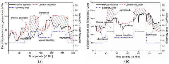
Figure 2. (a) Electricity generation of plant A in each period before and after optimization; (b) electricity generation of plant B in each period before and after optimization.

4.2. Electricity Purchasing Cost

The comparison of the electricity purchasing cost for plant A and plant B is shown in Table 2. The decreased electricity purchasing cost is the result of the optimal load management of the boilers under the TOU power price. Thus, the optimized management would result in daily electricity cost savings of approximately 0.15 million CNY for plant A and 0.53 million CNY for plant B, and would result in annual savings of 54 million CNY and 190.8 million CNY, respectively, if considering 360 calendar days of regular production per year.

Table 2. The comparison of the electricity purchasing cost for plant A and plant B.

Items	Plant A	Plant B
Manual operation (CNY)	431,191	2,607,736
Optimal calculation (CNY)	284,428	2,078,560
Reduction percentage	34.04%	20.30%

4.3. Gasholder Levels

The BFG holder was taken as an example to illustrate the gasholder level change before and after optimization, as shown in Figure 3. For manual operation, the BFG holder level in plant A was below the middle level. The 300,000 m³ BFG holder level in plant B was above the middle level and the 200,000 m³ BFG holder level in plant B was sometimes above and sometimes below the middle level. After optimization, the adjusting scope of these three BFG holders was 102.5%, 158.6%, and 90.2% larger than the manual operation, respectively. The gasholders collaborated more closely with the OSPP in the optimization results. Taking the 120,000 m³ BFG holder in plant A as an example, the holder level dropped (ending level minus starting level) for optimal calculation during two PPPs: T = 80–110 and T = 160–210 were 81,511 m³ and 76,509 m³, respectively. For manual operation, the corresponding holder level drops were only 4810 m³ and 19,565 m³, respectively, which demonstrated that the storage ability of the BFG holder was fully developed. In addition, the BFG holder adjusted more closely to the TOU power price after optimization.

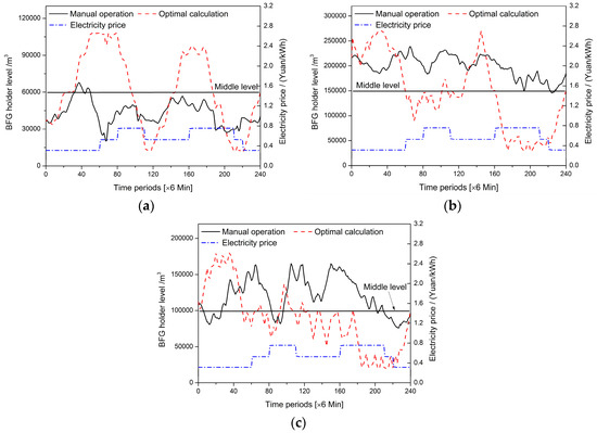
Figure 3. (a) Comparison of manual operation and optimal calculation results for the 120,000 m³ (Blast furnace gas) BFG holder of plant A; (b) comparison of manual operation and optimal calculation results for the 300,000 m³ (Blast furnace gas) BFG holder of plant B; (c) comparison of manual operation and optimal calculation results for the 200,000 m³ (Blast furnace gas) BFG holder of plant B.

4.4. Operation Strategy

Because the OSPP in plant A mainly consists of boilers and corresponding turbines, the priority of byproduct gas supply is given to high-efficiency boilers or boilers that are highly sensitive to operation load changes. However, for plant B, the thermal efficiency of CCPPs is much higher than the steam boilers and thus the priority of byproduct gas supply is given to CCPPs at all times. Only if the surplus volume of byproduct gases is very large and exceeds the maximum capacity of both 150 MW and 50 MW CCPPs will the two 130 t/h steam boilers consume the rest of the gases. Therefore, for the end users of steel plants, different operation strategies should be conducted according to their configurations of OSPPs. The proposed model can provide the optimal adjustment value for boilers, CCPPs, and gasholders in each scheduling period, which helps the decision maker to operate the byproduct gas system. The goal is to achieve economic benefits and improve the overall efficiencies of the OSPPs.

5. Conclusions

This paper proposed an MILP-based optimal scheduling model of byproduct gases in steel plants concerning the time-of-use (TOU) power price. Of special emphasis is the discussion on the load shifting potential of on-site power plants (OSPP). The peak-valley shifting of the electricity generation was better realized in the proposed scheduling model. Calculation results demonstrate that the electricity purchasing can be reduced by 34.04% and 20.30% for plant A and plant B, respectively, which is important for production cost reduction in the steel industry. In addition, the future energy systems in steel plants could fully develop their flexibility in power generation to balance the fluctuated power demand in the main grid. The proposed model has also good potential to be applied in real practice, especially for energy intensive industries with on-site power generation units and energy storage units.

References

- Consumption of Electricity and Its Main Varieties by Sector. Available online: http://data.stats.gov.cn/english/easyquery.htm?cn=C01 (accessed on 10 April 2017).
- Liu, J.; Cai, S.; Chang, Y. Economic benefit between autonomous power and purchasing power from state grid in iron and steel enterprises. J. Northeast. Univ. 2015, 36, 980–984. (In Chinese) [Google Scholar]
- Zhao, X.; Bai, H.; Shi, Q.; Lu, X.; Zhang, Z. Optimal scheduling of a byproduct gas system in a steel plant considering time-of-use electricity pricing. Appl. Energy 2017, 195, 100–113. [Google Scholar] [CrossRef]
- Kong, H.; Qi, E.; Li, H.; Li, G.; Zhang, X. An MILP model for optimization of byproduct gases in the integrated iron and steel plant. Appl. Energy 2010, 87, 2156–2163. [Google Scholar] [CrossRef]
- Yang, J.; Cai, J.; Liu, J.; Sun, W. Supply-demand forecast of byproduct gas system and optimized allocation of surplus gas. J. Northeast. Univ. 2015, 36, 1125–1129. (In Chinese) [Google Scholar]
- Porzio, G.F.; Nastasi, G.; Colla, V.; Vannucci, M.; Branca, T.A. Comparison of multi-objective optimization techniques applied to off-gas management within an integrated steelwork. Appl. Energy 2014, 136, 1085–1097. [Google Scholar] [CrossRef]
- He, K.; Zhu, H.; Wang, L. A new coal gas utilization mode in China’s steel industry and its effect on power grid balancing and emission reduction. Appl. Energy 2015, 154, 644–650. [Google Scholar] [CrossRef]
- Zeng, Y.; Sun, Y. Short-term Scheduling of Steam Power System in Iron and Steel Industry under Time-of-use Power Price. J. Iron Steel Res. Int. 2015, 22, 795–803. [Google Scholar] [CrossRef]
- Zhao, X.; Bai, H.; Lu, X.; Shi, Q.; Han, J. A MILP model concerning the optimisation of penalty factors for the short-term distribution of byproduct gases produced in the iron and steel making process. Appl. Energy 2015, 148, 142–158. [Google Scholar] [CrossRef]
- Zhao, X.; Bai, H.; Li, H.; Wang, C.; Zheng, L.; Han, J. Dynamic optimal distribution model of surplus byproduct gases in iron and steel making process. Chin. J. Eng. 2015, 37, 97–105. [Google Scholar]
- Zhang, X.; Zhao, J.; Wang, W.; Cong, L.; Feng, W. An optimal method for prediction and adjustment on byproduct gas holder in steel industry. Expert Syst. Appl. 2011, 38, 4588–4599. [Google Scholar] [CrossRef]
- Maneschijn, R.; Vosloo, J.C.; Mathews, M.J. Investigating load shift potential through the use of off-gas holders on South African steel plants. In Proceedings of the International Conference on the Industrial and Commercial Use of Energy (ICUE), Cape Town, South Africa, 17–19 August 2015. [Google Scholar]
- Li, T.; Castro, P.M.; Lv, Z.M. Life cycle assessment and optimization of an iron making system with a combined cycle power plant: A case study from China. Clean Technol. Environ. Policy 2016, 19, 1–13. [Google Scholar] [CrossRef]
- Hadera, H.; Harjunkoski, I. Continuous-time Batch Scheduling Approach for Optimizing Electricity Consumption Cost. Comput. Aided Chem. Eng. 2013, 32, 403–408. [Google Scholar]
- Zhu, Q.; Luo, X.; Zhang, B.; Chen, Y. Mathematical modelling and optimization of a large-scale combined cooling, heat, and power system that incorporates unit changeover and time-of-use electricity price. Energy Convers. Manag. 2016, 133, 385–398. [Google Scholar] [CrossRef]
- Gong, C.; Tang, K.; Zhu, K. An optimal time-of-use pricing for urban gas: A study with a multi-agent evolutionary game-theoretic perspective. Appl. Energy 2016, 163, 283–294. [Google Scholar] [CrossRef]
- Liu, J.; Cai, J. An Optimization Model Based on Electric Power Generation in Steel Industry. Math. Probl. Eng. 2014, 8, 1–10. [Google Scholar] [CrossRef]
- Azadeh, M.; Michael, F. Transition of Future Energy System Infrastructure; through Power-to-Gas Pathways. Energies 2017, 10, 1089. [Google Scholar]
- Kim, J.H.; Yi, H.S.; Han, C. A novel MILP model for plant-wide multi-period optimization of byproduct gas supply system in the iron and steel making process. Chem. Eng. Res. Des. 2003, 81, 1015–1025. [Google Scholar] [CrossRef]
© 2017 by the authors. Licensee MDPI, Basel, Switzerland. This article is an open access article distributed under the terms and conditions of the Creative Commons Attribution (CC BY) license (http://creativecommons.org/licenses/by/4.0/).