Abstract
The large-scale integration of electric vehicles (EVs) into power systems is expected to lead to challenges in the operation of the charging infrastructure. In this paper, we deal with the problem of an aggregator coordinating charging schedules of EVs with the objective of minimizing the total charging cost. In particular, unlike most previous studies, which assumed constant maximum charging power, we assume that the maximum charging power can vary according to the current state of charge (SOC). Under this assumption, we propose two charging schemes, namely non-preemptive and preemptive charging. The difference between these two is whether interruptions during the charging process are allowed or not. We formulate the EV charging-scheduling problem for each scheme and propose a formulation that can prevent frequent interruptions. Our numerical simulations compare different charging schemes and demonstrate that preemptive charging with limited interruptions is an attractive alternative in terms of both cost and practicality. We also show that the proposed formulations can be applied in practice to solve large-scale charging-scheduling problems.
1. Introduction
The ongoing transformation of modern energy systems around the world entails increasing, large-scale integration of electric vehicles (EVs). However, this poses challenges for the operation of the power system and the charging infrastructure, such as voltage variation, transformer lifespan reduction, and congestion-related problems [1,2,3]. EVs’ negative impacts on the power grid can be significantly mitigated by coordinating and controlling the charging behavior of EVs. This is possible because most EV users are indifferent about how charging rates vary during the charging process, as long as the EVs can be charged to their target levels by the desired departure time.
Coordination and control of aggregated charging load can be performed by an aggregator or a charging operator, which is a central entity acting as an interface between EV users and the system operator or electricity market [4]. The aggregator can provide the power grid with regulation services by increasing or decreasing charging rates in response to grid conditions, thereby helping to maintain stability. The aggregator could also be a for-profit entity and thus might try to reduce charging costs by distributing the aggregated charging load appropriately so that the charging amount increases as much as possible when the electricity price is relatively low. The for-profit aggregator could also determine energy retail prices as means to indirect load control [5]. The benefits obtained from such charging management can be shared between the aggregator and EV users. Therefore, it is important for the aggregator to take various charging-process and EV-user constraints into account when designing algorithms for optimal charging control.
In this paper, we envision a scenario wherein a charging station is operated by a single aggregator that coordinates and controls the charging schedules of all EVs subscribing under pre-determined payment schemes. The aggregator procures electricity from the electricity market (e.g., day-ahead, intraday, or balancing market) based on the EV charging-load forecasts and real-time charging-load fluctuations. He then optimizes the EV charging schedule centrally based on collected EV information such as arrival time, deadline, current state of charge (SOC), and desired SOC. The aggregator optimizes the charging schedule to minimize the total charging cost while satisfying all EVs’ charging requirements. The EV users can benefit from the implementation of such optimized charging control by sharing part of the saved charging costs with the aggregator. Consideration of this business model, however, is not within the scope of the present paper; rather, we focus on the optimization of EV charging scheduling and the objective of minimizing charging costs from the perspective of the aggregator.
Coordination and control of EV charging has been much studied over the past few years. Most work has modeled EV charging scheduling in the forms of optimization problems with different objectives. Many studies have focused on the total charging-cost-minimization problem from the perspective of EV users [6,7,8,9]. Some other investigations have focused on grid operator problems such as the minimization of distribution system losses [2] and the maximization of a valley-filling effect [10]. Various aggregator problems, meanwhile, also have been studied. Wu et al. [11] proposed EV-scheduling algorithms that aggregators can use to maximize energy-trading profits in the wholesale electricity market. In [12], the problem of finding optimal bid volumes and prices for the day-ahead market was solved, and in [13], a novel charging strategy for a smart charging station was proposed. Jin et al. [14], with the objective of aggregator-profit maximization, studied the problem of the optimization of an EV charging schedule with energy storage in the electricity market. In [15], distributed optimization algorithms for valley filling and charging-cost-minimization problems were proposed.
The structure of the EV charging-scheduling problem is highly dependent on the given charging schemes. In the literature, most papers assume a continuous charging scheme under which the EV can vary its charging rate continuously between zero and its maximum charging rate ([1,7,13,16,17], etc.). However, in practice, EVs are more likely to be charged at discrete charging rates. Several works have considered problems under the assumption that the EVs are charged at a constant charging rate [18,19,20,21,22]. In [19,20,21], the EV charging-scheduling decision was reduced to the determination of EV charging start times under the assumption that the charging process is uninterruptible. By contrast, Refs. [18,22] considered the case where the charging process can be interrupted. In this case, the problem is to decide whether to charge or not for each time period for each EV. Furthermore, in [23], the authors addressed a finite set of available charging rates.
There are two different approaches to the control of EV charging: centralized charging [2,11,14,24,25,26] and decentralized charging [13,15,20,27]. In centralized charging control, the aggregator determines the charging scheduling of all EVs. Information on the overall EV charging requirement usually is sent to the aggregator, who performs the schedule optimization accordingly. In decentralized charging control, the decision on the charging scheduling of each EV is made by each EV, while some communication between the aggregator and the EV is needed for coordination of the charging schedules of all EVs.
The previous work on EV charging scheduling also can be classified by the optimization techniques used to solve problems. To that end, traditional mathematical programming approaches, including linear programming [6,28], nonlinear programming [15,29], mixed-integer programming [14], and dynamic programming [23], have been extensively applied. Some other studies have also utilized meta-heuristic algorithms including genetic algorithm [30], particle swarm optimization [8], simulated annealing [31], and others. Still other approaches include game theory [32], queueing theory [33], and multi-agent systems [34], among others. For a detailed review of EV charging scheduling, the reader is referred to [35,36].
The main focus of this study is to schedule a large number of single-aggregator-subscribing EVs in such a way that minimizes the total charging cost from the aggregator perspective. Accordingly, the charging control considered in this paper can be classified as aggregator-based centralized charging control. As for the charging scenario, we focus on realistic charging schemes that take into account variable maximum charging power. Note that most work in the literature assumes that the maximum charging power is fixed over time. In reality, the typical lithium-ion-battery charging profile that most EVs employ has variable maximum charging power that normally is dependent on the current SOC. To be specific, the maximum charging power usually decreases as the battery level approaches full charge. Therefore, consideration of variable maximum charging power is necessary so as to reflect current practice. Under the assumption of variable maximum charging power, we consider two charging schemes: non-preemptive and preemptive charging. Under both schemes, the EV is charged according to a pre-determined profile, but the difference between the two is that preemptive charging allows interruptions during the charging process, whereas non-preemptive charging does not. For both charging schemes, we propose mathematical formulations of the EV charging-scheduling problem. Our formulations can deal with any charging profiles provided that the charging power can be represented as a function of the SOC.
The contributions of our study are as follows:
- We consider the aggregator’s EV charging-scheduling problem under the assumption of variable maximum charging power.
- We propose mathematical formulations for two different charging schemes: non-preemptive and preemptive charging.
- We also introduce an adaptation of the proposed formulation as a way of preventing frequent interruptions in the charging process.
- Our numerical simulations compare the different charging schemes and demonstrate that preemptive charging with limited interruptions is an attractive alternative in terms of both cost and practicality.
- We also show that our formulation is computationally efficient in solving practical, large-scale charging-scheduling problems.
This paper is organized as follows. Section 2 describes the EV charging scenario considered in this paper. The formulations of the EV charging scheduling problem under variable maximum charging power are given in Section 3. The results of our numerical simulations are presented and discussed in Section 4, and our conclusions are summarized in Section 5.
2. Scenario Description
2.1. Aggregator Settings
We consider the scenario in which a single aggregator operates a charging station that might be located in commercial or residential parking lots and controls the charging of all EVs that subscribe to the aggregator. We assume a discretized charging horizon with finite time periods () within which the EVs () start and finish charging. In practice, the duration of each time interval () is given as an hour or 15 min, which correspond to the time intervals at which the electricity price is determined in the electricity markets. We also assume that the electricity price changes depending on time (e.g., time-of-use (TOU) or real-time pricing), which encourages the aggregator to minimize charging costs by optimizing charging schedules. Let denote the electricity price at time t. In this paper, we assume that the electricity price can be estimated precisely in advance. Recently, there has been a growing literature investigating centralized EV charging scheduling problems under stochastic electricity prices [9,12]. Other sources of uncertainty such as EV charging demand and renewable supply have also been considered [24,25,26].
In addition, for the aggregator, let denote the maximum allowable charging load at time t, which can have different meanings depending on the way the aggregator operates the charging station: it could be the amount of power the aggregator purchased at the day-ahead market—or the aggregator could also make a contract with the utility company for the maximum amount of power that can be used for each time period. can also be given by the system operator according to the overall load information of the distribution grid and can vary over time to help achieve valley filling.
The aggregator, prior to executing the optimization process, collects information on each EV’s charging requirement. We assume that EV v informs the aggregator that it arrives at time with initial battery level and leaves the charging station at time with desired battery level . We denote as the set of time periods during which EV v can be charged.
2.2. Variable Maximum Charging Power
We consider the case wherein the maximum charging power can vary over time. In practice, it is common to charge EVs according to pre-determined charging profiles once the charging process starts. Such charging profiles are determined in consideration of the maximum charging power, which is expressed as a function of the SOC of the EV and is usually not constant. For example, the SOC curve shown in Figure 1 represents how the maximum charging power of a typical lithium-ion EV battery changes according to the current SOC [7]. Basically, the maximum charging power decreases slowly when the SOC is relatively low and starts to decrease rapidly as the SOC approaches its limit. Under such an SOC curve, a typical lithium-ion-battery charging profile can be approximated as shown in Figure 2a [37]. As indicated, charging power is treated as a function of the SOC. Note that it is also assumed that the EV is charged at constant power until the SOC reaches a certain level , after which the charging power decreases to zero as the SOC approaches full charge. The charging power of this charging profile can also be represented as a function of the elapsed time using a piecewise linear function, as shown in Figure 2b, which we call a piecewise linear charging profile. Most of the studies in the literature have adopted the assumption of the fixed maximum charging power for reasons of simplicity, and therefore assume that actual charging power can vary between 0 and the maximum at any time. However, such an assumption, because it neglects current practice, can produce sub-optimal or infeasible charging schedules.
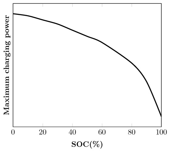
Figure 1.
SOC curve.
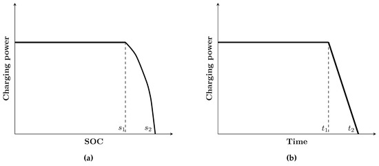
Figure 2.
Piecewise linear charging profile: (a) function of SOC; and (b) function of time.
For this study, we adopted a piecewise linear charging profile, since most EVs nowadays use lithium-ion batteries, the charging power of which is determined by the current SOC. However, the mathematical formulations we propose in this paper can be used for any charging profiles, provided that the charging power can be represented as a function of the current SOC or elapsed time; in any case, we will restrict our attention herein to the piecewise linear charging profile. Given this charging profile, we propose two different charging schemes: non-preemptive charging and preemptive charging.
2.3. Charging Schemes
Under the non-preemptive charging scheme, the EV is charged without interruptions once the charging starts. An example of non-preemptive charging scheduling under the piecewise linear charging profile is illustrated in Figure 3a, where the EV is charged at constant power (3.5 kW) for six consecutive hours after which, for the next two hours, the charging power is decreased (3 kWh and 1 kWh of energy are charged) to a charge total of 25 kWh. Note that the duration of each time interval is given as an hour. It is also important to note that, once the charging start time is determined, the charging power for each time period can be known a priori. Similarly, for any given charging profiles, we can produce discretized charging schedules for a fixed charging start time.
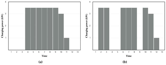
Figure 3.
Examples of charging schedules: (a) non-preemptive charging; and (b) preemptive charging.
In non-preemptive charging, the aggregator is supposed to control only the starting time, as the charging scheduling depends only on the charging start time, which restricts flexibility in charging control. In order to increase the charging flexibility, therefore, we additionally allow interruptions during the charging process, which leads to the preemptive charging scheme. Figure 3b depicts an example of preemptive charging, which incorporates two interruptions into the charging schedule of Figure 3a. We can see that the number of time periods during which the EV is charged and the charging power for such time periods is the same as those for non-preemptive charging. From a technology standpoint, the preemptive charging requires additional on-off switchings to interrupt the on-going charging process. However, frequent interruptions may introduce extra deterioration for batteries or threaten the stability of distribution transformer [22]. In order to overcome these limitations, we adapt our formulation in such a way that prevents frequent interruptions.
3. Problem Formulation
In this section, we propose mathematical formulations of the EV charging-scheduling problem under two charging schemes, non-preemptive charging and preemptive charging. Note that, in order to increase readability of the formulations, given parameters and sets are denoted by capital letters while decision variables and indexes are denoted by lower case letters.
3.1. Non-Preemptive Charging
As mentioned in the previous section, if interruptions during the charging process are not allowed, once the charging start time is determined, the charging power for each time period can be calculated automatically. The non-preemptive charging problem then, thus reduced to determining the charging start times of the EVs, can be developed as
where the binary variable takes value 1 if EV v starts its charging at time t, and 0 otherwise. Constraints (2) ensure that EV v must start charging between its arrival and departure time. Constraints (3) impose an upper bound on the aggregated charging power at time t, where represents the charging power of EV v at time t when the charging is started at time s. Note that the additional continuous variable represents the excess charging power required to satisfy the total charging requirements at time t. Finally, objective (1) minimizes the total charging cost over a planning horizon. It should be noted that is the unit cost needed to procure additional power exceeding the maximum allowable charging load at time t. For example, could be the electricity price in the balancing market if the aggregator purchases of power from the day-ahead market with the price and also procures additional power from the balancing market. If the aggregator has his own generator, could be the unit cost needed to procure additional power using self-generation. The constant in the objective represents the total charging cost of EV v that starts the charging at time t and can be calculated a priori.
3.2. Preemptive Charging
Formulating the EV charging-scheduling problem for preemptive charging is not as straightforward as for non-preemptive charging, since the amount of charging power at a certain time period is represented as a function of the SOC at the outset of the time period. Therefore, it is necessary to include variables representing the SOC at each time period as well as those representing whether EVs are charged for each time period or not. For an EV v, let be the number of different SOC values that it can take at the beginning and end of each time period, and let . Then, the k-th SOC value that EV v can take is denoted by . Note that and , i.e., initial and final SOC of EV v. Finally, the amount of charging power when the starting SOC value is is denoted by , which can be determined a priori according to a given charging profile. The idea of the formulation is that, for each EV, we assign one of the different SOC values to each time period in such a way that when k-th SOC value is assigned to time t, (k + 1)-th SOC value is assigned to time t + 1 if the EV is charged at time t and the SOC value remains unchanged at time t + 1 if the EV is not charged at time t. With the notation defined, the mathematical formulation for the preemptive charging case can be developed as
The binary variable takes value 1 if EV v is charged at time t, and 0 otherwise. The continuous variable represents the actual charging power of EV v at time t. Note that it takes value 0 if EV v is not charged at time t. The binary variable takes value 1 if EV v takes the k-th SOC value at the outset of time t, and 0 otherwise. Then, the values of the variable representing the SOC value of EV v at the outset of time t and the variable representing the charging power of EV v at time t if it is charged are both determined by . The meaning of the variable should not be confused with that of the variable . The variable represents the amount of charging power needed to charge EV v if it is charged at time t while represents the actual charging power of EV v at time t and thus can have value 0 if it is not charged. Constraints (6)–(8) state that the SOC value and the charging power of each time period must take one of the predetermined SOC values and charging powers. Constraints (9) and (10) together determine actual charging power () of each EV by enforcing the relation between the variables and : if , and if . Note that in the constraints represents the upper limit of charging power for EV v. Constraint (11) describes the relation of the SOC values for two consecutive time periods.
The formulation PCP can be quite large and impractical when the number of EVs and time periods is large. For this reason, we propose the extended formulation PCP-E, which makes use of a transition network defined for each EV, a path of which corresponds to a feasible charging schedule. We expect that the resulting formulation will enable us to reduce computation time, since optimization solvers are expected to exploit the intrinsic network structure of the formulation.
Prior to developing the extended formulation, let us first associate a transition network to each EV v by which the charging schedule of the EV can be visualized. Nodes in the network are defined by a pair , where t defines the time period and k defines the SOC level ranging from 1 to , the number of different SOC levels. The transitions between nodes are of two types:
- Charging transition : EV v with SOC level k at the outset of time t is charged during time t,
- Idle transition : EV v with SOC level k at the outset of time t is not charged during time t.
In this transition network, a path from node to node constitutes a feasible charging schedule of EV v, which is to say, a charging schedule that can charge the required power no later than the deadline set by the EV user. Note that the charging power associated with the charging transition → can be calculated a priori because we know the SOC value of the EV battery when the EV is at node (). Figure 4 graphically illustrates the possible transitions associated with node of a certain EV.
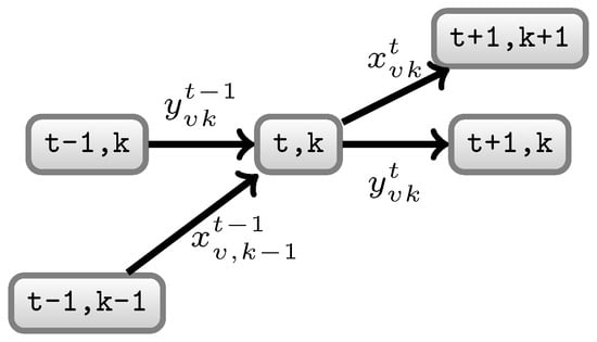
Figure 4.
Transitions associated with node .
A path in a transition network can be modeled via network flow by making use of the property such that, for each node, the number of transitions entering and leaving the node is always the same [38]. We now develop the extended formulation of the charging-scheduling problem under the preemptive charging scheme by modeling network flow on the transition networks. We associate binary variables and with each of the two types of transition. The variable takes value 1 if EV v with SOC level k at the outset of time t is charged during time t, and 0 otherwise. The variable takes value 1 if EV v with SOC level k at the outset of time t is not charged during time t, and 0 otherwise. The formulation PCP-E can then be developed as
here, objective (15) is to minimize the total charging costs over a planning horizon, where represents the charging power of EV v if it is charged during a certain time period from SOC level k. Constraints (16) enforces maximum limits on the total charging load at each time period. Constraints (17)–(19) represent flow conservations at each node in the transition networks. Note that constraints (18) and (19) correspond to flow conservation at the source and sink nodes, respectively. Finally, the integrality of variables is imposed by constraints (20).
A feasible solution to PCP-E constitutes paths on each transition network, which, in turn, yields feasible charging schedules of each EV. Conversely, we can also derive, from the given feasible charging schedule, feasible paths in each transition network. This leads to the following proposition.
Proposition 1.
The formulation PCP-E is equivalent to the formulation PCP.
3.3. Controlling Frequency of Interruption
Although preemptive charging provides additional flexibility relative to non-preemptive charging, in practice, it might be desirable to avoid frequent interruptions during the charging process, as they require additional on/off control. Frequent interruptions can also shorten the lifespan of a battery [19]. In order to prevent frequent interruptions in the charging schedule, we can adapt our formulation by introducing the following additional cost term to objective (15):
where is a penalty parameter of EV v for not charging during time period t. Note that we penalize the transition → such that k is between 2 and , meaning that the time periods during which the EV is not charged are penalized after the EV starts charging until the EV finishes charging. The resulting charging schedule becomes closer to the non-preemptive charging schedule as we increase the penalty parameter , which will be shown in detail in the numerical experiments of the following Section 4.
4. Numerical Simulations
In this section, we report the results of our numerical simulations comparing the two different charging schemes proposed in this paper and also testing the computational performances of the proposed formulations. All of the tests were performed on a 3.1-GHz Intel Core i7 processor with 16 GB RAM. We solved all of the formulations using Xpress 8.0 with the default parameter settings.
4.1. Simulation Settings
We consider a time horizon of 17 h from 5:00 p.m. to 10:00 a.m. the next day, and we assume that each time period is one hour. The hourly electricity price is the actual day-ahead price of PJM Interconnection from 1 July to 30 July of 2016 [39]. We assume that all EVs have a battery capacity of 25 kWh and are charged following the piecewise linear charging profile, under which an EV is charged with a charging rate of 3.5 kW for the first 6 h, 2.97 kW for the 7th hour, and 1.03 kW for the last hour, if it is charged from zero battery level [37]. The initial SOC is assumed to follow a uniform distribution from 0 to 12 kWh, which implies that each EV requires a different time for charging depending on the initial SOC. We also assume that all EVs want to fully charge their battery (i.e., the desired SOC is 25 kWh for all EVs). The arrival time of each EV is assumed to follow a normal distribution with a mean of 7:00 p.m. and a standard deviation of 1 h, and the departing time is also assumed to follow a normal distribution with a mean of 8:00 a.m. and a standard deviation of 1 h.
4.2. Results and Discussion
We first compared the computational performance of the formulations PCP and PCP-E developed for the preemptive charging problem; the results are shown in Table 1. We solved two formulations for 18 sets of instances by varying the number of EVs ( = 500, 1000, 1500, 2000, 2500, and 3000) and the maximum allowable hourly charging load ( = 1.2, 1.5, and 1.8 MWh). For each set, we generated 10 different instances by randomly generating the arrival time, departure time, and initial SOC of each EV using the probability distribution introduced above; thus, each row in the table reports the average, minimum, and maximum solution times over those ten instances. The hourly electricity price corresponds to that for 1 July 2016. A time limit of five minutes (300 s) was imposed on each instance. From the table, we can see that PCP-E was able to solve all of the tested instances within approximately 15 s and that PCP was able to solve all but one tested instance within the limit of 300 s, which demonstrates that PCP-E is much faster than PCP. This might be due to the fact that the optimization solver was able to detect the intrinsic network structure of PCP-E and therefore to take advantage of it in solving large-sized mixed integer programming problems. As the formulation PCP-E proved to be efficient in solving the preemptive charging problem up to 3000 EVs, it is expected that it will prove to be a practical means of solving the large-scale charging-scheduling problem.

Table 1.
Comparison of solution times (in seconds) between two formulations.
We next compared the two charging schemes, non-preemptive charging and preemptive charging, in terms of the total charging cost. To do this, for each of six different numbers of EVs ranging from 500 to 3000, we randomly generated EV information such as arrival time, departure time, and initial SOC. We then solved the formulations NCP and PCP-E for six generated instances by varying the maximum allowable hourly charging load ( = 1.2, 1.5, and 1.8 MWh) and the hourly electricity price data from 1 July to 30 July 2016. Therefore, we solved a total of instances. The results are shown in Table 2. In the table, each row presents the average, minimum, and maximum total charging costs over 30 instances, each of which corresponds to one of 30 days. We can see that preemptive charging yields a smaller total charging cost than does non-preemptive charging, since the former provides for more charging flexibility. The average cost reduction achieved due to allowing interruptions amounted to 1.49–3.72% of the total charging cost of non-preemptive charging. We also observed that such cost reductions decreased as the maximum allowable hourly charging load increased. This trend can be explained by the fact that when the maximum charging load is sufficient, charging schedules are likely to be already optimized enough and thereby leave little room for cost reduction from interruptions.
Table 2.
Comparison of total charging costs (in thousand dollars) between non-preemptive and preemptive charging schemes.
Figure 5 plots the total charging costs as a function of the duration of time interval . Note that the charging flexibility can be increased by reducing the duration of each time interval, since it is equivalent to having more decisions to make on whether to charge an EV or not for each time period. To see how total charging costs change, we solved a randomly generated instance with 50 EVs for different values and price data. The meaning of the abbreviations that are used in the figure is summarized as follows:
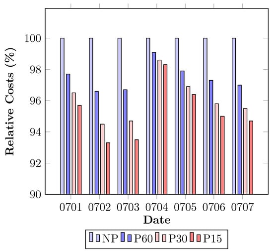
Figure 5.
Total charging cost as a function of time interval duration.
- NP: Non-preemptive charging,
- P60: Preemptive charging with = 60 min,
- P30: Preemptive charging with = 30 min,
- P15: Preemptive charging with = 15 min.
We plotted the results corresponding to each price data from 1 July to 7 July 2016, and we represented the total charging costs as the percentage relative to the total charging cost of NP. We can observe that reducing the duration of each time interval leads to a decrease in total charging costs. However, such an impact on cost reduction diminishes as the time interval duration is reduced. Specifically, the average cost reductions over 30 days achieved from “P60”, “P30”, and “P15” relative to the cost of NP were 2.63, 3.97 and 4.72%, respectively. Figure 6 shows how the EV charging schedule is influenced by charging schemes and the time interval duration, which depicts the charging schedules of a certain EV among 50 EVs. Note that the obtained charging schedules are all depicted on an hourly basis for the purpose of comparison. It can be easily observed that charging flexibility increases by allowing interruptions, thereby further decreasing the time interval duration.
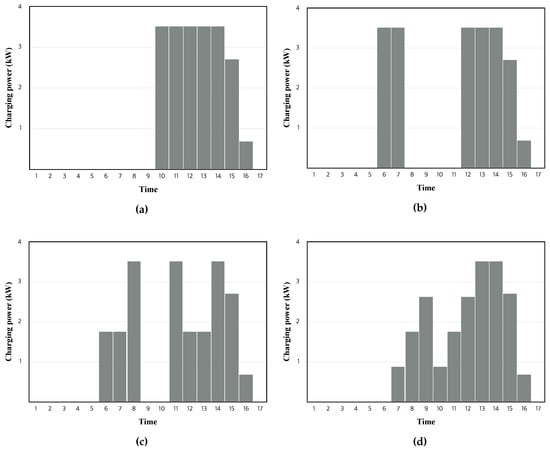
Figure 6.
Examples of charging schedules corresponding to different charging schemes: (a) non-preemptive charging; (b) preemptive charging with = 60 min; (c) preemptive charging with = 30 min; and (d) preemptive charging with = 15 min.
As mentioned in the previous section, increased charging flexibility is accompanied by additional charging controls that could be complicated and lead to additional costs. For this reason, we introduced a simple modification of the proposed formulation PCP-E that can be used to control the frequency of interruptions in the obtained charging schedule. We now present results indicating how effective such a modification is in reducing the number of interruptions in preemptive charging. We solved an randomly generated instance with 50 EVs for different penalty parameters and price data. The results are shown in Table 3, where the x in the heading refers to the formulation PCP-E with and x has the values 0, 0.5, and 1. The average number of interruptions and the average total charging costs over 30 days are reported for each penalty parameter value. We can see that the average number of interruptions decreases with the increase of the penalty parameter. This decrease also results, as was expected, in the increase of the total charging cost. Note, however, that the number of interruptions per EV is already small (0.76 on average), even when the penalty parameter is not imposed, which is to say, when . A notable finding is the fact that the number of interruptions was reduced by approximately 32% with only a 0.04% increase of total charging cost. This demonstrates the highly significant impact of the introduction of our penalty parameter.
Table 3.
Effect of penalty parameter on number of interruptions and total charging costs (in dollars): The penalty parameter is given as .
5. Conclusions
In this paper, we investigated the EV charging-scheduling problem from the perspective of an aggregator who centrally coordinates and controls the charging behavior of all connected EVs so as to minimize total charging costs. Our main contribution to the existing literature is our development of mathematical formulations of the EV charging-scheduling problem under the assumption that maximum charging power can vary depending on the SOC of the EV battery. We considered two charging schemes: non-preemptive and preemptive charging. The latter allows interruptions during the charging process, whereas the former does not. In particular, preemptive charging can provide more charging flexibility than non-preemptive charging, although it can cause more charging control. We proposed an extended formulation for the preemptive charging problem, along with a modification to enable control of the frequency of interruptions. Our computational simulation demonstrated that the proposed extended formulation is solved quickly for large-scale instances and therefore can be used for practical purposes. As for the cost comparison between the charging schemes, it was shown that preemptive charging can reduce the total charging cost of non-preemptive charging by 1.5–3.7% for the tested instances, and that the total charging cost also can be reduced by decreasing the duration of each time interval. Finally, we showed that the number of total interruptions in the charging schedule can be reduced considerably with only a small increase of total charging cost, which can be achieved by adding penalty terms to the formulation. Therefore, our major finding is that the preemptive charging schedule with limited interruptions can be an attractive choice in terms of both cost and practicality.
Acknowledgments
This work was supported by the National Research Foundation of Korea (NRF) grant funded by the Korea government (MSIP) (No. 2017R1C1B2006144). This work was supported by Basic Science Research Program through the National Research Foundation of Korea (NRF) funded by the Ministry of Education (NRF-2015R1D1A1A01057719). The authors also thank the Institute for Industrial Systems Innovation of Seoul National University for the administrative support.
Author Contributions
Jinil Han proposed the mathematical formulations, designed the simulations, and wrote the paper; Jongyoon Park performed the simulations and analyzed the results; and Kyungsik Lee conceived the structure and the research direction of the paper.
Conflicts of Interest
The authors declare no conflict of interest.
References
- Clement-Nyns, K.; Haesen, E.; Driesen, J. The impact of charging plug-in hybrid electric vehicles on a residential distribution grid. IEEE Trans. Power Syst. 2010, 25, 371–380. [Google Scholar] [CrossRef]
- Sortomme, E.; Hindi, M.M.; MacPherson, S.J.; Venkata, S. Coordinated charging of plug-in hybrid electric vehicles to minimize distribution system losses. IEEE Trans. Smart Grid 2011, 2, 198–205. [Google Scholar] [CrossRef]
- Clement, K.; Haesen, E.; Driesen, J. Coordinated charging of multiple plug-in hybrid electric vehicles in residential distribution grids. In Proceedings of the 2009 IEEE/PES Power Systems Conference and Exposition, Seattle, WA, USA, 15–18 March 2009; pp. 1–7. [Google Scholar]
- Bessa, R.J.; Matos, M.A. The role of an aggregator agent for EV in the electricity market. In Proceedings of the 7th Mediterranean Conference and Exhibition on Power Generation, Transmission, Distribution and Energy Conversion (MedPower 2010), Agia Napa, Cyprus, 7–10 November 2010; pp. 1–9. [Google Scholar]
- Momber, I.; Wogrin, S.; San Román, T.G. Retail pricing: A bilevel program for PEV aggregator decisions using indirect load control. IEEE Trans. Power Syst. 2016, 31, 464–473. [Google Scholar] [CrossRef]
- He, Y.; Venkatesh, B.; Guan, L. Optimal scheduling for charging and discharging of electric vehicles. IEEE Trans. Smart Grid 2012, 3, 1095–1105. [Google Scholar] [CrossRef]
- Cao, Y.; Tang, S.; Li, C.; Zhang, P.; Tan, Y.; Zhang, Z.; Li, J. An optimized EV charging model considering TOU price and SOC curve. IEEE Trans. Smart Grid 2012, 3, 388–393. [Google Scholar] [CrossRef]
- Saber, A.Y.; Venayagamoorthy, G.K. Resource scheduling under uncertainty in a smart grid with renewables and plug-in vehicles. IEEE Syst. J. 2012, 6, 103–109. [Google Scholar] [CrossRef]
- Korolko, N.; Sahinoglu, Z. Robust Optimization of EV charging schedules in unregulated rlectricity markets. IEEE Trans. Smart Grid 2017, 8, 149–157. [Google Scholar] [CrossRef]
- Zhang, K.; Xu, L.; Ouyang, M.; Wang, H.; Lu, L.; Li, J.; Li, Z. Optimal decentralized valley-filling charging strategy for electric vehicles. Energy Convers. Manag. 2014, 78, 537–550. [Google Scholar] [CrossRef]
- Wu, D.; Aliprantis, D.C.; Ying, L. Load scheduling and dispatch for aggregators of plug-in electric vehicles. IEEE Trans. Smart Grid 2012, 3, 368–376. [Google Scholar] [CrossRef]
- Vayá, M.G.; Andersson, G. Optimal bidding strategy of a plug-in electric vehicle aggregator in day-ahead electricity markets under uncertainty. IEEE Trans. Power Syst. 2015, 30, 2375–2385. [Google Scholar] [CrossRef]
- You, P.; Yang, Z.; Chow, M.Y.; Sun, Y. Optimal Cooperative Charging Strategy for a Smart Charging Station of Electric Vehicles. IEEE Trans. Power Syst. 2016, 31, 2946–2956. [Google Scholar] [CrossRef]
- Jin, C.; Tang, J.; Ghosh, P. Optimizing electric vehicle charging with energy storage in the electricity market. IEEE Trans. Smart Grid 2013, 4, 311–320. [Google Scholar] [CrossRef]
- Rivera, J.; Goebel, C.; Jacobsen, H.A. Distributed convex optimization for electric vehicle aggregators. IEEE Trans. Smart Grid 2017, 4, 1852–1863. [Google Scholar] [CrossRef]
- Gan, L.; Topcu, U.; Low, S.H. Optimal decentralized protocol for electric vehicle charging. IEEE Trans. Power Syst. 2013, 28, 940–951. [Google Scholar] [CrossRef]
- de Hoog, J.; Alpcan, T.; Brazil, M.; Thomas, D.A.; Mareels, I. Optimal charging of electric vehicles taking distribution network constraints into account. IEEE Trans. Power Syst. 2015, 30, 365–375. [Google Scholar] [CrossRef]
- Han, S.; Han, S.; Sezaki, K. Development of an optimal vehicle-to-grid aggregator for frequency regulation. IEEE Trans. Smart Grid 2010, 1, 65–72. [Google Scholar]
- Gan, L.; Topcu, U.; Low, S.H. Stochastic distributed protocol for electric vehicle charging with discrete charging rate. In Proceedings of the Name of the Power and Energy Society General Meeting, San Diego, CA, USA, 22–26 July 2012; pp. 1–8. [Google Scholar]
- Binetti, G.; Davoudi, A.; Naso, D.; Turchiano, B.; Lewis, F.L. Scalable real-time electric vehicles charging with discrete charging rates. IEEE Trans. Smart Grid 2015, 6, 2211–2220. [Google Scholar] [CrossRef]
- Beaude, O.; Lasaulce, S.; Hennebel, M.; Mohand-Kaci, I. Reducing the Impact of EV Charging Operations on the Distribution Network. IEEE Trans. Smart Grid 2016, 7, 2666–2679. [Google Scholar] [CrossRef]
- Sun, B.; Huang, Z.; Tan, X.; Tsang, D.H. Optimal Scheduling for Electric Vehicle Charging with Discrete Charging Levels in Distribution Grid. IEEE Trans. Smart Grid 2016. [Google Scholar] [CrossRef]
- Rotering, N.; Ilic, M. Optimal charge control of plug-in hybrid electric vehicles in deregulated electricity markets. IEEE Trans. Power Syst. 2011, 26, 1021–1029. [Google Scholar] [CrossRef]
- Xu, Y.; Pan, F. Scheduling for charging plug-in hybrid electric vehicles. In Proceedings of the 2012 IEEE 51st Annual Conference on Decision and Control (CDC), Maui, HI, USA, 10–13 December 2012; pp. 2495–2501. [Google Scholar]
- Huang, Q.; Jia, Q.S.; Qiu, Z.; Guan, X.; Deconinck, G. Matching EV charging load with uncertain wind: A simulation-based policy improvement approach. IEEE Trans. Smart Grid 2015, 6, 1425–1433. [Google Scholar] [CrossRef]
- Xu, Y.; Pan, F.; Tong, L. Dynamic Scheduling for Charging Electric Vehicles: A Priority Rule. IEEE Trans. Autom. Control 2016, 61, 4094–4099. [Google Scholar] [CrossRef]
- Vayá, M.G.; Andersson, G.; Boyd, S. Decentralized control of plug-in electric vehicles under driving uncertainty. In Proceedings of the Innovative Smart Grid Technologies Conference Europe (ISGT-Europe), Istanbul, Turkey, 12–15 Octomber 2014; pp. 1–6. [Google Scholar]
- Sortomme, E.; El-Sharkawi, M.A. Optimal combined bidding of vehicle-to-grid ancillary services. IEEE Trans. Smart Grid 2012, 3, 70–79. [Google Scholar] [CrossRef]
- Yao, W.; Zhao, J.; Wen, F.; Xue, Y.; Ledwich, G. A hierarchical decomposition approach for coordinated dispatch of plug-in electric vehicles. IEEE Trans. Power Syst. 2013, 28, 2768–2778. [Google Scholar] [CrossRef]
- Talebizadeh, E.; Rashidinejad, M.; Abdollahi, A. Evaluation of plug-in electric vehicles impact on cost-based unit commitment. J. Power Sources 2014, 248, 545–552. [Google Scholar] [CrossRef]
- Valentine, K.; Temple, W.G.; Zhang, K.M. Intelligent electric vehicle charging: Rethinking the valley-fill. J. Power Sources 2011, 196, 10717–10726. [Google Scholar] [CrossRef]
- Ma, Z.; Callaway, D.S.; Hiskens, I.A. Decentralized charging control of large populations of plug-in electric vehicles. IEEE Trans. Control Syst. Technol. 2013, 21, 67–78. [Google Scholar] [CrossRef]
- Li, G.; Zhang, X.P. Modeling of plug-in hybrid electric vehicle charging demand in probabilistic power flow calculations. IEEE Trans. Smart Grid 2012, 3, 492–499. [Google Scholar] [CrossRef]
- Vandael, S.; Boucké, N.; Holvoet, T.; De Craemer, K.; Deconinck, G. Decentralized coordination of plug-in hybrid vehicles for imbalance reduction in a smart grid. In Proceedings of the Name of the 10th International Conference on Autonomous Agents and Multiagent Systems, Taipei, Taiwan, 2–6 May 2011; pp. 803–810. [Google Scholar]
- Mukherjee, J.C.; Gupta, A. A review of charge scheduling of electric vehicles in smart grid. IEEE Syst. J. 2015, 9, 1541–1553. [Google Scholar] [CrossRef]
- Yang, Z.; Li, K.; Foley, A. Computational scheduling methods for integrating plug-in electric vehicles with power systems: A review. Renew. Sustain. Energy Rev. 2015, 51, 396–416. [Google Scholar] [CrossRef]
- Zhang, P.; Qian, K.; Zhou, C.; Stewart, B.G.; Hepburn, D.M. A methodology for optimization of power systems demand due to electric vehicle charging load. IEEE Trans. Power Syst. 2012, 27, 1628–1636. [Google Scholar] [CrossRef]
- Ahuja, R.K.; Magnanti, T.L.; Orlin, J.B. Network Flows: Theory, Algorithms, and Applications; Prentice-Hall, Inc.: Upper Saddle River, NJ, USA, 1993; ISBN 0-13-027765-7. [Google Scholar]
- PJM. PJM Power Market, 2016. Available online: http://www.pjm.com (accessed on 30 October 2016).
© 2017 by the authors. Licensee MDPI, Basel, Switzerland. This article is an open access article distributed under the terms and conditions of the Creative Commons Attribution (CC BY) license (http://creativecommons.org/licenses/by/4.0/).