Abstract
The thermal conductivity of soils and rocks constitutes an important property for the design of geothermal energy foundations and borehole heat exchange systems. Therefore, it is interesting to find new alternatives to define this parameter involved in the calculation of very low enthalpy geothermal installations. This work presents the development of an experimental set-up for measurements of thermal conductivity of soils and rocks. The device was designed based on the principle of the Guarded Hot Plate method using as heat source a laboratory heater. The thermal conductivity of thirteen rocky and soil samples was experimentally measured. Results are finally compared with the most common thermal conductivity values for each material. In summary, the aim of the present research is suggesting a procedure to determine the thermal conductivity parameter by a simple and economic way. Thus, increases of the final price of these systems that techniques such as the “Thermal Response Test” (TRT) involvs, could be avoided. Calculations with software “Earth Energy Designer” (EED) highlighted the importance of knowing the thermal conductivity of the surrounding ground of these geothermal systems.
1. Introduction
With respect to the lithosphere, heat transfer is produced by thermal conduction; heat diffuses without transfer of matter. Conduction is the principal mechanism of thermal propagation that takes part in the process of thermal exchange in a very low temperature geothermal installation [1].
Thus, the parameter of thermal conductivity (W/mK) plays a fundamental role in these systems. When this value increases, the capacity of the ground to transmit the heat to the components of the installation is also bigger, increasing its efficiency. Therefore, thermal conductivity constitutes a reference to evaluate the speed of the energetic extraction through the geothermal pipes or the dissipation of heat through the ground. For these reasons, it is recommendable to define this parameter to carry out a suitable calculation of a low enthalpy geothermal installation [2,3,4].
There are many different ways to measure this thermal property. Generally, experimental methods can be grouped into two categories: (i) stable methods, which provide more precise results despite requiring long measurement periods; and (ii) non-stable methods, which stand out for their rapidity, although they offer a lower precision.
Regarding the geothermal field, in practice, tables providing reference values of thermal conductivity for a set of materials are commonly used. In such cases, only approximate values are used, so the calculation of the installation may not be completely correct. This fact usually causes over-measurements that, in some cases, involve considerable increases of the final cost [5,6].
In large projects, another less frequent practice is the execution of a “Thermal Response Test” (TRT) that allows obtaining “in situ” the thermal conductivity parameter. The test allows studying the behavior of the ground when a constant thermal power is transmitted through the geothermal pipe. It constitutes a suitable solution in spite of the high cost that its realization implies, especially in small installations where a TRT could mean an important increase of the global budget.
Laboratory studies of the thermal conductivity of soils and rocks are usually carried out on samples collected from the ground.
The “Guarded Hot Plate” (GHP) method is the standard technique for measuring thermal conductivity of solid materials in the range from about 0.01 to 15 W/mK [7]. Two main versions of the GHP method can be differentiated: the double-sided (2S-GHP) which implies the use of two identical specimens, and the single-sided (1S-GHP) that only uses one specimen. Different techniques based on this method are used in the laboratory to measure the thermal conductivity of rocky and soil samples [8].
Ramstad et al. [9] designed equipment to measure the thermal diffusivity of rock samples. Thermal conductivity was calculated as a product of density, specific heat capacity and thermal diffusivity. Lira-Cortés et al. [10] implemented a system of thermal conductivity measurement for solid conductive materials. The system measured the thermal conductivity of an aluminum bar using a reference material.
Liou and Tien [11] estimated the thermal conductivity of granite using a combination of techniques, the “Transient Plane Source” (TPS) method [12], the thermal probe method and heat transfer test.
Krishnaiah et al. [13] designed a thermal probe to estimate different thermal properties such as thermal resistivity and diffusivity, and specific heat of rocks.
Kukkonen and Lindberg [14] measured the thermal conductivity of rocks making use of the steady-state divided bar method.
Jorand et al. [15] used the TCS method based on contact-free thermal conductivity scanning of a plane or cylindrical surface [16]. This instrument uses a focused, mobile and continuously operating heat source, together with two infrared temperature sensors at small distances behind and in front of the source, for measuring the thermal conductivity along scanning lines.
Table 1 presents a comparison among the works previously cited and the method proposed in the present study.

Table 1.
Contributions and limitations of past thermal conductivity works.
As examples of more recent studies, Xiao et al. [17] proposed an analytical model for effective thermal conductivity of nanofluids, while Cai et al. [18] provide a complete review about the recent investigations on the fractal models and fractal-based approaches applied for effective thermal conductivity.
Devices commercially produced to measure this property are numerous at present. As example, the equipment commercially known as KD2-PRO is commonly used to determine the thermal conductivity of different materials including rocks and soils [19,20]. However, most of the equipment is not cheap and the price of the whole geothermal system immediately grows.
The present research offers a description of a thermal conductivity measuring apparatus based on the 1S-GHP (a single-sided guarded hot plate) principle. The aim is to present a new alternative to estimate this parameter making use of usual equipment in a soil science laboratory: a laboratory heater. Throughout this work, we describe a new experimental application of the 1S-GHP method; we apply the method to a set of heterogeneous rocks and soil samples; and we compare these values with the theoretical ones.
The novelty of this study is the combination of both rocks and soils thermal conductivity measurements in the same device. The main strength of the method is the simplicity in the calculation of the thermal conductivity parameter by measuring temperatures in four horizons. The measurement range reaches the thermal conductivity of aluminum, used as reference sample in the current work.
2. Materials and Methods
2.1. Description of the Suggested Method
In the laboratory of Rock Mechanics of the Higher Polytechnic School of Avila (Spain), a procedure to determine the thermal conductivity of different samples of rocks and soils was developed.
The method suggests, from two pattern samples (SR1-SR2) with well-known value of thermal conductivity, quantifying this property in any other sample (S) whose value of thermal conductivity wants to be known. A heat source (laboratory heater) that generates a constant heat flow Qx, was used. This flow goes through the three samples (SR1-S-SR2) placed contiguous as shown in Figure 2. Temperatures are controlled in four horizons (T1, T2, T3, and T4) by thermocouples (Figure 1). Once these temperatures are stabilized and known, they can be used in the corresponding calculation of the thermal conductivity parameter [21,22].
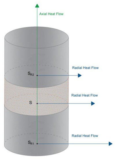
Figure 2.
Heat flux distribution.
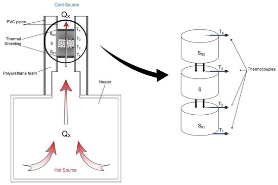
Figure 1.
Schema of the suggested method.
The cold source equally schematized in Figure 1 represents the temperature of the room where the measurement equipment was placed. It is important to highlight that this cold source was kept constant during the whole process of measurement, given that any variation could involve important changes in the results. Thus, the temperature of the cold source was controlled and set in the value of 296.65 K.
2.2. Theoretical Basis
In the system described in Figure 1, the transfer of heat only occurs by conduction with one-dimensional flux and permanent state. The possible convection phenomena were prevented placing two aluminum sheets that behaved as insulations. The action of these sheets made the thermal transfer among the different samples purely conductive. Thermal conductivity is the physical property that controls the conduction of heat in a solid. It is materialized by Fourier’s law (Equation (1)) which relates the specific heat flow and the gradient of temperature [23,24,25]:
where = Heat flux in the direction x; k = Thermal conductivity; A = Area of the transverse section of the conductive object; and = Gradient of temperature in the direction x.
If we apply Equation (1) to each one of the samples that are part of the system, the resultant equations are:
Heat flux was calculated using temperatures T1, T2, T3 and T4 (when they become steady) and Equation (1). This calculation was possible because of two main facts: the heat flux is constant and thus the same for each of the samples, and we use two reference samples with known thermal conductivity values (SR1 and SR2).
From value and considering the steady temperatures, the dimensions of sample S and Equation (1), thermal conductivity of the sample S can be easily calculated [26,27].
Therefore, by the implementation of the procedure detailed in the present paper, it is viable to obtain the value of thermal conductivity of a particular material S.
Equations (1) and (2) can be obtained based on Fourier’s law. Heat transport in geo-materials is known of dual-phase-lagging type. It is important to mention that Fourier’s law of heat conduction is valid only for some limiting cases, so the method will be limited to those situations.
2.3. Heat Flux Analysis
Until now, the heat flux has been considered as one-dimensional; it only flows in the longitudinal direction. However, after several tests and temperatures analysis, it was experimentally verified that, in spite of the insulation used, there was an additional heat flux in radial direction.
Analyzing temperatures T1, T2, T3 and T4, it was observed that, through the first pattern sample SR1, a substantial quantity of heat flux is lost as radial flux. As a result, sample SR1 was not used in the corresponding thermal conductivity calculations (it was only used as a stabilizing element of the system). The location of this sample minimizes the loss of heat as radial flux in the remaining samples (S and SR2).
Nonetheless, axial heat flux in samples S and SR2 must also be considered, because, although smaller, it alters the final results too. To quantify this radial flux, the method was previously used on a sample with known thermal conductivity value. Once this flux was quantified, final thermal conductivity results were exempt from this kind of error.
The distribution of the heat flow is represented in Figure 2.
2.4. Equipment Description
The device designed to measure the thermal conductivity parameter consists of the following components:
- Sterilization and drying heater “Dry-Big” (Figure 3):
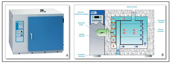 Figure 3. (A) Heater outside view; and (B) heater internal schema.Heater with air force circulation mechanism, regulated by a microprocessor and with temperature and time digital reading. It constitutes the heat source used for the calculation of the thermal conductivity parameter.A set of working temperatures was tested to analyze the evolution of the thermal conductivity with the temperature. Thus, heat source was regulated according to the most suitable temperature.
 - PVC pipes (Figure 1):Two PVC hollow cylinders were used in the construction of the equipment.
- Hollow cylinder of diameter slightly higher to the air outlet placed on the top of the heater. This PVC pipe of diameter (0.10 m) coupled to the air outlet was adiabatically insulated in the whole contour by polyurethane foam.
- Hollow cylinder 0.052 m of diameter, placed inside the previous pipe. It behaves as fastener of the samples. The space between both pipes was adiabatically insulated by polyurethane foam.
- Polyurethane foam (Figure 1):Polyurethane foam was used to insulate the system from any external influence getting at the same time one-dimensional circulation of the heat flux through the samples.It is a porous plastic material made up of a bubble aggregation. It consists of the chemical reaction of two polyol and isocyanate, although it accepts multiple additives. Its insulation capacity comes from the low thermal conductivity of the gas that its closed cells send.
- Pattern samples (Figure 2):Two reference samples with known thermal conductivity values were used. These samples are made of pure aluminum. Given the high thermal conductivity of this element, it facilitates the heat flux transmission through the system. The dimensions of both patterns are: 0.10 m of thickness and 0.05 m of diameter.
- Thermocouples (Figure 1):Four sounding lines (constituted by chrome and aluminum alloys) connected to a digital thermometer made possible the measurement of temperatures in four areas. Before its use, thermocouples were duly calibrated [28].
As explained in Section 2.2, calculations of the thermal conductivity parameter can only be carried out when the four temperatures recorded by the thermocouples keep a constant value over time. Figure 4 shows a graphical example of readings of these sounding lines. After a certain period of time, thermocouples record constant temperature values; these data are the ones used in the calculation of the thermal conductivity of sample S.
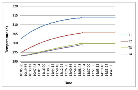
Figure 4.
Measuring of temperatures with thermocouples.
First, the PVC pipe of 0.1 m was coupled to the heater air outlet. A central opening was left for the subsequent placement of the second PVC pipe. Space between the first pipe and the opening was filled with polyurethane foam. A pattern sample (SR1) followed the sample whose conductivity wants to be measured (S) and the other pattern sample (SR2) was introduced in the second pipe. After placing thermocouples in the corresponding horizons, the second pipe was placed in the central opening to begin the test.
3. Methodology of the Thermal Conductivity Test
The methodology of the proposed thermal conductivity test includes the next stages.
3.1. Materials Selection
A series of materials (rocks and soil) were selected to carry out the thermal conductivity measurements. These materials have different composition and nature so the study covers a varied geological range, defining with more precision the reliability of the methodology in question.
Table 2 shows the materials used in the study.
Table 2.
Materials selected for the test.
3.2. Samples Preparation
Samples used to test the thermal conductivity equipment, required a specific preparation whether they are rocks or soils.
3.2.1. Rocky Samples
Rocky samples are cylindrical blocks of 0.05 m in diameter and variable thickness. The preparation of these samples was carried out as follows:
Sample extraction (Figure 5): Using a rotating drilling machine equipped with diamond circular crown, it was possible to obtain cylinder blocks of each of the rocky materials. The diameter of these blocks was of 0.05 m and variable thickness depending on the size of the origin rock. During the process of extraction, the crown was cooled by water.
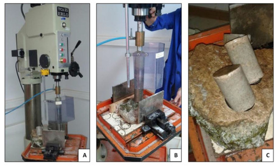
Figure 5.
Sample extraction: (A) rock placing; (B) drilling; and (C) final samples.
Carving of samples (Figure 6): Cylinder samples were cut using a cutting-machine supplied with diamond disk to give the samples a certain thickness. Samples of different thickness were prepared, with the aim of analyzing the influence of this factor in the calculation of the thermal conductivity. Thickness of each one of the samples was measured by electronic caliber.
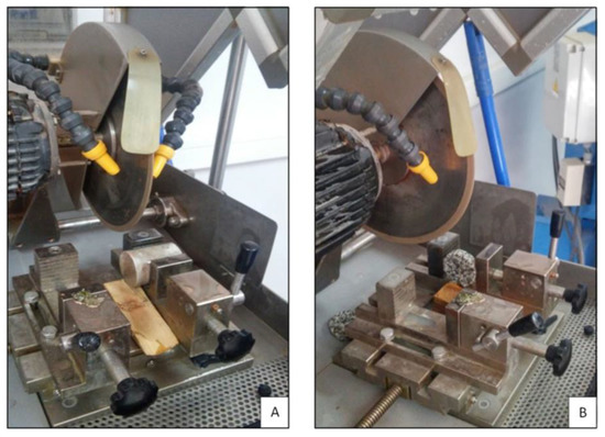
Figure 6.
(A) Cutting of a quartzite sample; (B) Cutting of a granitic sample.
Samples cleaning: Samples surfaces were thoroughly cleaned to minimize any possibility of error at the heat transmission. It facilitates the contact with the temperature sounding lines or thermocouples. Figure 7 shows the final appearance of some of these samples.
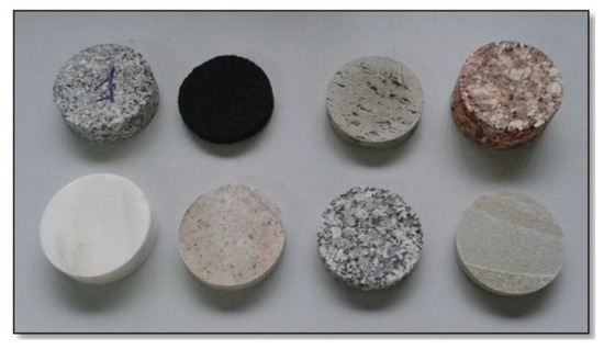
Figure 7.
Samples ready to be used in the suggested equipment.
3.2.2. Soil Samples
Soils materials followed a different procedure to equally get cylinder blocks of 0.05 m in diameter and variable thickness. The preparation of these samples was made according to the next steps.
Determination of humidity by drying in heater [29]: Thermal conductivity depends on the water content that a certain material has, thus, it is important to know the humidity conditions when measuring this parameter. Natural humidity of the soil at its origin was increased by adding a particular percentage of water. The addition of water facilitates the soil compaction in a mold to obtain cylinder samples that will be introduced into the measuring equipment.
Humidity was set to 11.55%.
Soil compaction: As already explained, the proposed system works with cylinder blocks of certain dimensions. Given that, in the case of soils, the material cannot be cut as rocks, it was compacted in a suitable mold. This compaction made easier the obtaining of cylinder samples ready for use in the thermal conductivity device
Soil compaction was made according to the Proctor Test conditions, in the point of the optimal humidity defined in the mentioned law [30].
3.3. Placing of Samples in the Measuring Equipment and Determination of Thermal Conductivities
Firstly, one of the aluminum reference samples SR1 was introduced in the carrier pipe, then sample S (whose thermal conductivity value wants to be measured) and finally the second aluminum reference sample SR2. It is important to highlight that, before the first reference sample and after the second one, two thin aluminum sheets were placed. The function of these sheets is to get a shielding that avoids convection phenomena. In this way, all the heat transfer just happens by thermal conduction.
Once placed the respective samples and thermocouples in the thermal conductivity equipment, it starts working, sending a constant heat flux that goes through the samples. After letting enough time to make the stabilization of temperatures T1, T2, T3 and T4, possible, the last step was making the correspondent calculations (as explained by the Section 2.2). Finally, thermal conductivities values of each of the samples were obtained.
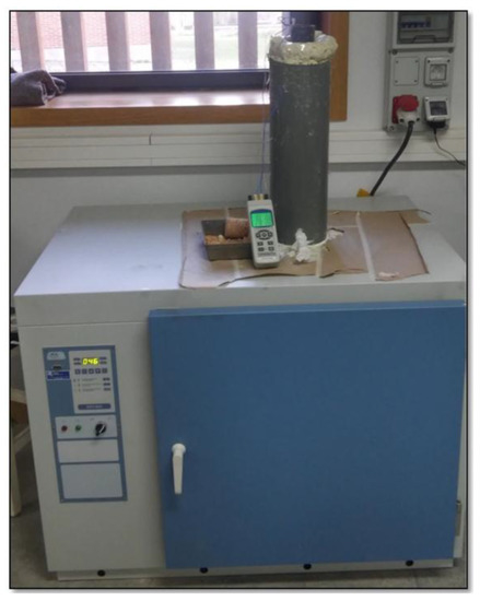
Figure 8.
Equipment designed to measure thermal conductivities.
4. Analysis of the Measuring Process
Before the measuring of the thermal conductivity parameter in different materials, a series of tests were carried out on the same rocky sample (granite). They were used to analyze how the thermal conductivity changes with the heater temperature and the thickness of the sample in question (S).
These tests allowed the establishment of the appropriate working conditions (temperature of the heat source and sample thickness) to be used in the subsequent measuring of thermal conductivities of the samples presented in Table 2.
4.1. Evolution of the Thermal Conductivity with Temperature
In a crystalline solid, thermal conductivity depends on temperature; however, this dependence is not homogeneous. This dependence can be divided in four regions, so the variation of conductivity will be different based on the region where it is. In region I, of low temperature (T ≤ 20 K), thermal conductivity quickly increases with temperature, being proportional to T3. In region II, it achieves a maximum value, usually at a temperature close to T ≈ θD/20 (where θD is the Debye’s temperature). At higher temperatures, in region III, thermal conductivity decreases proportionally to T−1. Finally, at very high temperatures (T ≥ θD) in region IV, it stops being dependent on temperature [31,32].
In this particular case, to analyze the behavior of the thermal conductivity with the temperature, the region where the present study is must be defined. To that end, in the first place, Debye’s temperature was determined. Table 3 shows the values of Debye’s temperatures for a series of substances.
Table 3.
Debye’s temperatures for a series of substances.
The substance in Table 3 with the most similar composition to the studied material (granite) is silica. It has a Debye’s temperature of 645 K, so that, if T ≈ 645 K/20 = 32.25 K, in this value, thermal conductivity will get its maximum value and will decrease at higher temperatures until the point of T ≥ 645 K where it starts being independent of temperature. Therefore, the assumption studied is in region III, which establishes an inversely proportional relation between temperature and thermal conductivity.
Figure 9 presents the distribution of the regions and the behavior that the system should have in the area where it is, region III.
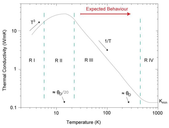
Figure 9.
Dependence of thermal conductivity with temperature for a crystalline solid.
Graphically, taking from the graphic in Figure 9 two temperatures and the corresponding values of thermal conductivity according to the curve represented in region III, it is possible to establish the reduction of thermal conductivity with the temperature in that region. Thus, if we select the temperatures of 95 K and 100 K, we can verify the decrease of thermal conductivity with an increase of temperature of 5 K. In this way, and according to Debye’s graphical, for the temperature of 95 K, the corresponding value of thermal conductivity is 2.01 W/mK, while for 100 K the value of thermal conductivity is 1.87 W/mK. It means that an increase of 5 K of temperature involves a reduction of thermal conductivity of 0.14 W/mK. That is to say, in a crystalline solid, per each grade of temperature increased, thermal conductivity decreases 0.028 W/mK.
Nevertheless, the granitic sample used to examine the variation of the thermal conductivity with the temperature, contains about 30% of silica. Thus, the reduction for this sample would not be of 0.028 W/mK (for a material constituted by 100% of silica), but 0.0084 W/mK per each grade of temperature increased in this material.
The above is the expected behavior of thermal conductivity based on theoretical knowledge. However, to know what really happens in the practice of this procedure, tests with this method were carried out at different working temperatures (313.15 K, 338.15 K and 358.15 K) and always with the same sample (granite whose content in silica is around 30%). It will allow determining the evolution of the thermal conductivity with these temperatures (Table 4).
Table 4.
Thermal conductivity for different values of temperature and sample thickness.
4.2. Variation of the Thermal Conductivity with the Sample Thickness
Another of the tests consisted in analyzing the variation of the thermal conductivity parameter with different thicknesses of the sample S. In this way, the range of sample thickness for which the equipment properly worked was established, discarding those ones where the results obtained moved away from the reference values. Thus, through these tests, the limits of the system regarding the sample thickness were set.
As in the previous case, a series of measurements were made with the same granitic sample modifying in this case its thickness.
The results of these tests (modifying the working temperatures and the sample thickness) are described in Table 4.
Analyzing the results presented in Table 4 and focusing on the variation of the working temperature, thermal conductivity was measured for three values of working temperature and for each of these cases, four thickness of the same granitic sample. Table 5 and Table 6 show the variation of the thermal conductivity for each thickness when the working temperature, increases from 313.15 K to 338.15 K and from 313.15 K to 338.15 K. Additionally, Table 5 and Table 6 present the decrease of the thermal conductivity parameter for each grade that the sample temperature increases.
Table 5.
Evolution of thermal conductivity when temperature increases from 313.15 K to 338.15 K.
Table 6.
Evolution of thermal conductivity when temperature increases from 338.15 K to 358.15 K.
Some deductions can be drawn:
- Most of the thermal conductivity values are around 2 W/mK. Increasing the temperature, these values decrease as it was expected for a crystalline solid. However, the reduction of the thermal conductivity parameter is not constant in the different sample thicknesses, and is not the expected 0.0084 W/mK calculated in Section 4.1. Evolution of thermal conductivity with temperature.Therefore, in a crystalline solid, thermal conductivity decreases when temperature grows. However, it was not possible to set a model of behavior of this reduction because it does not follow any constant pattern.
- Regarding the different sample thickness, Table 4 shows the measurements carried out at the laboratory equipment (four different thicknesses for each one of the three work temperatures). The optimal dimensions of the sample S could be established based on the results of these measurements.Thus, analyzing Table 4, it can be observed that, for the three temperatures, the values of thermal conductivity for each of the thickness are around the same value (~2 W/mK). These data agree with the expected thermal conductivity value for a granitic material. However, for the case of the highest thickness, the result of thermal conductivity moves away from the rest of results for lower thickness. All this made it possible to set the sample thicknesses for which the present method works properly.On the basis of these results, with sample thicknesses greater than 0.0131 m, the procedure described in this paper does not provide reliable values. In these cases, results are highly anomalous due to a high dissipation of the heat flux through the sample S.
- The following working conditions were established in the thermal conductivity apparatus:
- −
- Temperature of the heat source was set in 313.15 K. Although results were acceptable in the three temperatures (313.15 K, 338.15 K and 358.15 K), this value is closer to the ground temperature in a very low enthalpy geothermal installation.
- −
- Thickness of the sample S could not exceed in any case the mentioned 0.0131 m for the reasons previously justified.
5. Thermal Conductivity Results
The results of thermal conductivity measurements are presented in Table 7. Three measurements of this parameter were carried out on each of the samples considered.
Table 7.
Thermal conductivities, standard deviation and derivate error for each material studied.
When a certain measurement is repeated several times, medium values group around a central value. This distribution can be described by statistical the mean <x> (Equation (3)) and the standard deviation (Equation (4)) [33,34]:
Errors derived from the precision of the tools used to measure the different parameters (thickness and temperatures) must also be considered. For this reason, the total differential of our equation of calculation of conductivity was calculated (Equation (5)):
where
Equation (5) was transformed into increases, and absolutes values were taken to each partial derivate to estimate the derivate error (Equation (6)):
Increases represent the absolute errors of the measuring dispositive and the growth of k symbolizes the derivate error.
From each one of the three thermal conductivities measurements of each material, derivate error was calculated. It was found that the reduction in precision did not exceed in any case one order of magnitude with respect to the precision of the least precise dispositive (thermocouples with ±0.01 K). Derivate error was estimated as ±0.10 for all samples.
6. Validity of the Method
The validity of the suggested thermal conductivity device was analyzed by comparing the results presented in Table 7 with the ones commonly accepted at the “Technical Code of Building” (CTE). From this comparison, the difference, with respect to the officially accepted value for that sample, was calculated.
CTE provides a certain thermal conductivity value for a wide variety of materials, including rocks and soils. Given the heterogeneity of samples 1, 2, 3 and 4 (granitic rocks) and the high presence of these rocks in numerous European geothermal installations, a different reference value was assigned to each of these samples starting from the CTE value. This assignment was made based on studies that relate the thermal conductivity of a rock with its quartz content [35,36].
Thus, instead of the thermal conductivity value of 3 W/mK provided by the CTE for a granite rock, an interval of 2.0 W/mK–3.8 W/mK was taken for quartz contents between 3% and 50%.
Table 8 shows the reference thermal conductivity values set for each of the samples according to CTE. It also presents the thermal conductivity values measured with the equipment developed in this research and the difference between both values (common and measured values).
Table 8.
Comparison between values of thermal conductivity measured and the reference ones.
It is important to highlight that thermal conductivity parameter easily changes depending on different factors (temperature, anisotropy, humidity, etc.) and could be quite different in materials of similar geological origin. Despite these facts, the differences between the measured values and the reference ones are considerably low. The most unfavorable case was for sample 12 (0.37 W/mK of difference) and the most favorable one for sample 7 (0.01 W/mK of difference). Figure 10 shows a graphic of deviations presented in Table 8.
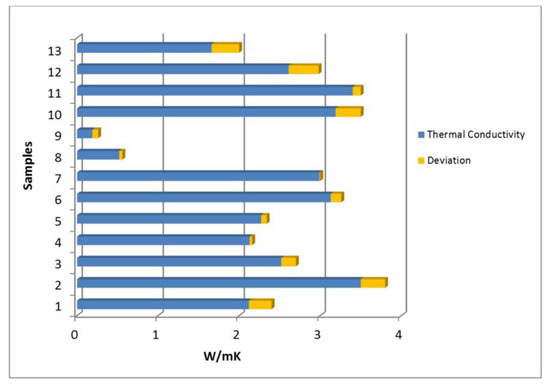
Figure 10.
Deviations between the common and the measured thermal conductivity values.
7. Influence of the Thermal Conductivity Parameter in the Geothermal Measuring
“Earth Energy Designer” (EED) is software developed by “Blocon Software” that allows knowing the total drilling depth of a vertical closed-loop system. The calculation process of EED is based on a series of initial data (provided by the user) of the ground where the installation is going to be placed. One of these initial data is the thermal conductivity of the surrounding ground.
In order to understand the importance that the thermal conductivity parameter has in the dimensioning of a geothermal installation, some calculations were made with this software. The total drilling depth was calculated with the same conditions but changing the thermal conductivity of the ground for each of the samples of this study. Thus, for each sample, calculations were made with the measured thermal conductivity value and with interval of ±15% of that value (Table 9).
Table 9.
Measuring with EED software.
Depending on the material, with a variation of only ±15% in the thermal conductivity value, the total drilling length significantly changes. The most notable case is sample 9, where increasing the thermal conductivity from 0.19 W/mK to 0.22 W/mK, the drilling length decreases 27 m, and reducing the thermal conductivity to 0.16 W/mK, the drilling length increases 34 m.
As Table 9 shows, for the rest of samples, large variations are also experimented. Therefore, a proper knowledge of the thermal conductivity of the ground means important variations in the total drilling depth of a very low enthalpy geothermal installation.
8. Conclusions
Thermal conductivity is a fundamental property in the process of measuring of a geothermal installation but, at the same time, it is a parameter of difficult quantification.
A series of difficulties of diverse nature appeared throughout this research:
- Temperature of the cold source (ambient temperature) was controlled at all times and set in a constant value to avoid external thermal influences on the thermal conductivity device.
- The insulation placed around the system minimized the radial heat flux but did not eliminate it. As a result, corrections of this heat flux were made for each of the temperatures set at the heater.
- A high precision was needed when measuring the sample thickness due to its excessive influence in the calculation of the thermal conductivity parameter.
- Thermocouples were carefully placed to ensure a complete contact with the faces of the samples.
- Long-term measurements to guarantee the stabilization of the heat flux.
Despite these facts, this method means an excellent solution when measuring the thermal conductivity parameter in an economical and simple way. It provides accurate results taking advantage of equipment present in most laboratories such as the heater. These results are applicable to the calculation of very low enthalpy geothermal installations, avoiding over measuring that raise the price of these renewable installations.
Finally, EED software allowed highlighting the importance of knowing the thermal conductivity of the surrounding ground in a geothermal system. This knowledge could mean important savings regarding the drilling length.
Acknowledgments
Authors would like to thank the Department of Cartographic and Land Engineering of the Higher Polytechnic School of Avila, University of Salamanca, for allowing us to use their facilities and their collaboration during the experimental phase of this research. Authors also want to thank the Ministry of Education, Culture and Sport for providing a FPU Grant (Training of University Teachers Grant) to the corresponding author of this paper what has made possible the realization of the present work.
Author Contributions
All authors conceived, designed and performed the experimental campaign. Cristina Sáez Blázquez, Arturo Farfán Martín and Ignacio Martín Nieto implemented the methodology and analyzed the results. Diego González-Aguilera provided technical and theoretical support. Cristina Sáez Blázquez wrote the manuscript and all authors read and approved the final version.
Conflicts of Interest
The authors declare no conflicts of interest.
References
- Leach, A.G. The thermal conductivity of foams. I: Models for heat conduction. J. Phys. D 1993, 26, 733–739. [Google Scholar] [CrossRef]
- Balbay, A.; Esen, M. Experimental investigation of using ground source heat pump system for snow melting on pavements and bridge decks. Sci. Res. Essays 2010, 5, 3955–3966. [Google Scholar]
- Balbay, A.; Esen, M. Temperature distributions in pavement and bridge slabs heated by using vertical ground-source heat pump systems. Acta Sci. Technol. 2013, 35, 677–685. [Google Scholar] [CrossRef]
- Kabar, M.; Nowak, W.; Sobanski, R. Principles of Exploitation Geothermal Energy Water at Targets of Heating Buildings; Project KBN; Energy Water at Targets of Heating Buildings: Szczecin, Poland, 1999. [Google Scholar]
- Blázquez, C.S.; Martín, A.F.; García, P.C.; Sánchez Pérez, L.S.; del Caso, S.J. Analysis of the process of design of a geothermal installation. Renew. Energy 2016, 89, 188–199. [Google Scholar] [CrossRef]
- Peláez, P.C.; Carnicero, J.M.P.; García, R.L.; Peragon, F.C. Desarrollo de equipo para la realización de test de respuesta térmica del terreno (TRT) en instalaciones geotérmicas. Dyna 2014, 89, 316–324. [Google Scholar] [CrossRef]
- ASTM International. ASTM Standard C 177-10, Standard Test Method for Steady-State Heat Flux Measurements and Thermal Transmission Properties by Means of the Guarded-Hot-Plate Apparatus; ASTM International: West Conshohocken, PA, USA, 2010. [Google Scholar]
- Terzic, M.; Miloševic, N.; Stepanic, N.; Petricevic, S. Development of a single-sided guarded hot plate apparatus for thermal conductivity measurements. Therm. Sci. 2016, 20, S321–S329. [Google Scholar] [CrossRef]
- Ramstad, R.K.; de Beer, H.; Midttømme, K.; Koziel, J.; Wissing, B. Thermal Diffusivity Measurement at NGU—Status and Method Development 2005–2008; Geological Survey of Norway: Trondheim, Norway, 2009. [Google Scholar]
- Lira-Cortés, L.; González Rodríguez, O.J.; Méndez-Lango, E. Sistema de Medición de la Conductividad Térmica de Materiales Sólidos Conductores, Diseño y Construcción; Simposio de Metrología Santiago de Querétaro: Querétaro, Mexico, 2008. [Google Scholar]
- Liou, J.-C.; Tien, N.-C. Estimation of the thermal conductivity of granite using a combination of experiments and numerical simulation. Int. J. Rock Mech. Min. Sci. 2016, 81, 39–46. [Google Scholar] [CrossRef]
- Gustafsson, S.E. Transient plane source techniques for thermal conductivity and thermal diffusivity measurements of solid materials. Rev. Sci. Instrum. 1991, 62, 797–804. [Google Scholar] [CrossRef]
- Krishnaiah, S.; Singh, D.N.; Jadhav, G.N. A methodology for determining thermal properties of rocks. Min. Sci. 2004, 41, 877–882. [Google Scholar] [CrossRef]
- Kukkonen, I.; Lindberg, A. Thermal Conductivity of Rocks at the TVO Investigation Sites Olkiluoto, Romuvaara and Kivetty; Report YJT-95-08, 29; Nuclear Waste Commission of Finnish Power Companies: Helsinki, Finland, 1995. [Google Scholar]
- Jorand, R.; Vogt, C.; Marquart, G.; Clauser, C. Effective thermal conductivity of heterogeneous rocks from laboratory experiments and numerical modeling. J. Geophys. Res. 2013, 118, 5225–5235. [Google Scholar] [CrossRef]
- Popov, Y.A. Optical scanning technology for nondestructive contactless measurements of thermal conductivity and diffusivity of solid matters. In Proceedings of the 4th World Conference on Experimental Heat Transfer, Fluid Mechanics and Thermodynamics, Brussels, Belgium, 2–6 June1997; pp. 109–116. [Google Scholar]
- Xiao, B.; Yang, Y.; Chen, L. Developing a novel form of thermal conductivity of nanofluids with Brownian motion effect by means of fractal geometry. Powder Technol. 2013, 239, 409–414. [Google Scholar] [CrossRef]
- Cai, J.; Hu, X.; Xiao, B.; Zhou, Y.; Wei, W. Recent developments on fractal-based approaches to nanofluids and nanoparticle aggregation. Int. J. Heat Mass Transf. 2017, 105, 623–637. [Google Scholar] [CrossRef]
- Blázquez, C.S.; Martín, A.F.; Nieto, I.M.; García, P.C.; Pérez, L.S.S.; Aguilera, D.G. Thermal conductivity map of the Avila region (Spain) based on thermal conductivity measurements of different rock and soil samples. Geothermics 2017, 65, 60–71. [Google Scholar] [CrossRef]
- Barry-Macaulay, D.; Bouazza, A.; Singh, R.M.; Wang, B.; Ranjith, P.G. Thermal conductivity of soils and rocks from the Melbourne (Australia) region. Eng. Geol. 2013, 164, 131–138. [Google Scholar] [CrossRef]
- ASTM International. ASTM D5334, Standard Test Method for Determination of Thermal Conductivity of Soil and Soft Rock by Thermal Needle Probe Procedure; ASTM International: West Conshohocken, PA, USA, 2008. [Google Scholar]
- ASTM International. ASTM E1225-99, Standard Test Method for Thermal Conductivity of Solids by the Guarded Comparative Longitudinal Heat Flow Technique; ASTM International: West Conshohocken, PA, USA, 1999. [Google Scholar]
- Jean-Baptiste, J.F. Remarques generales sur les temperatures du globe terrestre et des espaces plan etaires. Ann. Chim. Phys. 1824, 27, 136–167. [Google Scholar]
- Jean-Baptiste, J.F. Theorie Analytique de la Chaleur; Firmin Didot: Paris, France, 1822. [Google Scholar]
- Jean-Baptiste, J.F. Memoire sur les temperatures du globe terrestre et des espaces planetaires. Mem. l’Acad. R. Sci. 1827, 7, 569–604. [Google Scholar]
- Bevington, R.P.; Robinson, D.K. Data Reduction and Error Analysis for the Physical Sciences, 2nd ed.; WCB/McGraw-Hill: New York, NY, USA, 1992. [Google Scholar]
- Pei, W.; Yu, W.; Li, S.; Zhou, J. A new method to model the thermal conductivity of soil–rock media in cold regions: An example from permafrost regions tunnel. Cold Reg. Sci. Technol. 2013, 95, 11–18. [Google Scholar] [CrossRef]
- ASTM International. ASTM E220, Test Method for Calibration of Thermocouples by Comparison Techniques; ASTM International: West Conshohocken, PA, USA, 2013. [Google Scholar]
- AENOR. UNE 103-300-93. Determinación de la Humedad de un Suelo Mediante Secado en Estufa; AENOR: Marid, Spain, 1993. [Google Scholar]
- AENOR. UNE 103-500-94. Ensayo Proctor de Compactación; AENOR: Marid, Spain, 1994. [Google Scholar]
- Chung, P.W.; Tamma, K.K.; Namburu, R.R. Homogenization of temperature-dependent thermal conductivity in composite materials. J. Thermophys. Heat Transf. 2001, 15, 10–17. [Google Scholar] [CrossRef]
- Fernández, F.; Rondón, E.; Sánchez, F.; Salas, K.; García, V.; Briceño, J. Conductividad térmica en sólidos a altas temperaturas. Rev. Fac. Ing. UCV 2006, 21, 21–27. [Google Scholar]
- Nakshabandi, G.A.I.; Kohnke, H. Thermal conductivity and diffusivity of soils as related to moisture tension and other physical properties. Agric. Meteorol. 1965, 2, 271–279. [Google Scholar] [CrossRef]
- Taylor, R.J. An Introduction to Error Analysis: The Study of Uncertainties in Physical Measurements, 2nd ed.; University Science Books: Herndon, VA, USA, 1997. [Google Scholar]
- Kukkonen, I.; Lindberg, A. Thermal Properties of Rocks at the Investigation Sites: Measured and Calculated Thermal Conductivity. Specific Heat Capacity and Thermal Diffusivity; Geological Survey of Finland: Espoo, Filand, 1998. [Google Scholar]
- Prontuario de Soluciones Constructivas; Código Técnico de la Edificación; Instituto de Ciencias de la Construcción Eduardo Torroja e Instituto de Ciencias de la Construcción de Castilla y León: Castilla y León, Spain, 2007.
© 2017 by the authors. Licensee MDPI, Basel, Switzerland. This article is an open access article distributed under the terms and conditions of the Creative Commons Attribution (CC BY) license (http://creativecommons.org/licenses/by/4.0/).