Modelling and Optimization in Microgrids

Abstract

The expansion of renewable energies is progressing strongly. The influence on the power supply networks by the variability of the infeed must be met with new concepts. In this paper, we investigate the possibilities of integrating microgrids as a cooperating unit in the power supply network to support further expansion of renewable energy sources (RES) power plants. In this paper, a differentiation of microgrids from similar network structures is established, and a classification of proposed groups is made. Then, after the description of the simulation of the components in a microgrid, with practical advice, an example model is shown, which aids the dimensioning of the components within a microgrid to achieve a specified goal.

1. Introduction

The politically-promoted development of renewable energy sources (RES) in recent years is enormous. The breakdown of the RES plants by technology shows that wind energy (onshore) and photovoltaics are the most representative of the supplies in Europe [1]. The variability of energy supply by RES is a matter of concern and ongoing research. One of the studies on the variation of photovoltaics (PV) forecast in 2013 has shown that the average percentage of a day’s difference between forecast and gross annual average can be as high as 26.5% [2]. Variations in power generation and increasing harmonic distortion are the main problems related to PV systems [3].

The necessary network expansion proceeds very slowly due to very lengthy administrative approval processes. The addition of renewable energy sources, especially in the low-voltage network, however, is many times faster. Already, low voltage levels in some areas partly exceed the limits of permissible voltage differences according to EN 50160. Voltage dips, swells, transients and voltage harmonic content are the main issues [4,5]. The further construction of new renewable energy plants is therefore thwarted [6]. To ensure secure network operation, alternative concepts are therefore promoted. Microgrids represent a promising approach, acting as flexible, harmoniously cooperating cells of the power distribution system within the general context of smart grids.

The original idea of the microgrid presented in [7] is evolving: in this work, a microgrid can be defined as an association of sources, loads and storage that mutually compensate their outputs and are connected to a network node to the superimposed network as a harmoniously operating cell. Microgrids are able to smooth in this way the energy generated from volatile feeds and reproduce the defined load profile by appropriate control of the microgrid components, as proposed in [8]. Thus, also the forecast error will be minimized. Moreover, the construction of a microgrid can be done much more quickly than a network expansion, since the process for setting up a microgrid takes far less time and expense. Modelling and optimization of microgrids from the point of view of physics, system and control theory is shown in [9].

In [10], electric cars as a controllable load are considered together with the future potential of bidirectional operation. Electric vehicles’ (EV) grid interfacing is a challenging problem [9,10,11], as the simple load control fails when addressing issues that require a higher control level, such as managing congestion levels or enabling EVs to participate in the electricity markets. In [12], a similar concept of the balancing of local distribution grids with EV batteries is presented. In this paper, the simulation-based approach is applied to fully simulate a complex microgrid connected to a local medium voltage (MV) distribution grid, including charging stations and EVs.

Research related to the control of microgrids’ components, presented in [13,14], shows that the simulation-based approach is able to facilitate the evaluation of smart grid- and EV-related communication protocols, control algorithms for charging and the functionalities of local distribution grids as part of a complex, critical cyber-physical system. The resulting system can be applied to studying the balancing of local smart grids with EV batteries.

The main contributions of this paper lie in the presentation of practical considerations related to the operation and modelling of microgrids, the design of a complete framework for simulation and the optimization of a microgrid composed of photovoltaic generation, battery storage, combined heat and power (CHP) and an electrical vehicle charging pool. The flexible optimization approach to the components’ sizing is presented, as well. Most data are based on real measurements, recorded at a research facility.

The rest of the paper is organized as follows: the microgrid structures are described in Section 2, with differences presented in Section 3. In Section 4, the classification of microgrids into practically useful groups is justified, and in Section 5, the simulation aspects and recommendations are presented. In Section 6, the interconnections within microgrids are discussed, and in Section 7 and Section 8, an example of the simulation and optimization task is shown. The discussion of the results and concluding remarks is provided in Section 9.

2. Microgrid Structure

Similar to the smart grid architectural model (SGAM), a recognized architecture for independent analysis in the field of smart grids based on system layers, we adopt here an analogous treatment of microgrids [15].

2.1. Component Layer

The base of the microgrid is the component layer that contains the usual components of a network infrastructure: loads, generators and storage. Depending on the desired load characteristics, it is possible to curb individual consumers, if necessary, to increase or to reschedule the demand to a relevant time. Renewable energy producers as PV and wind turbines are only influenced by the energy supply and cannot be controlled in their feed. Cogeneration, biomass plants and diesel generators are also to be found in microgrids. The most common storage technology is the battery storage in the form of lead-acid or lithium-ion cells.

2.2. Communication Layer

Inside a microgrid, the interaction of individual subcomponents becomes essential. An interaction of the components can only be achieved through a comprehensive communication architecture. Due to various system components, communication media and manufacturers’ standards, the definition of interoperable system becomes essential. At the same time, one should consider the criteria, such as security, scalability, reliability, data protection, etc. The proven Internet IPv4 and IPv6 protocols offer in this regard a good solution. However, lack of data protection in the standard Internet protocols must be addressed by the application of special solutions. A further challenge is the collection of power consumption data from end users of the electrical energy. The Programmable Logic Controller (PLC) technology is an emerging technology for data transfer in low voltage power networks, however vulnerable to harmonic distortion.

2.3. Information Layer

This ensures the data processing based on the communication layer, standardized data models and a set of required data for each system component. The Standard 61850 provides definitions and models for substation automation as used in Supervisory Control and Data Acquisition (SCADA) systems.

2.4. Application Layer

This controls the operation of the microgrids. On this level operates the intelligent energy management system, a central control unit that interacts with the communication and component layer.

2.5. Business Layer

The top layer of the selected display employs the incentive schemes for an intelligent load management and marketing of the services provided by the microgrid control energy, but has to be compliant also with political and regulatory conditions.

3. Differences between Microgrid and Similar Network Structures

3.1. Standalone Grid

The standalone grid describes a spatially-delimited, autonomous power supply system, not permanently coupled to the public network. It contains internal loads, its own generation plants and energy storage. A stand-alone grid therefore is delimited primarily from the microgrid by a (permanently) non-available public grid work access. The comparatively low extent of the network leads to an increased load sensitivity, whereby above-average voltage and frequency fluctuations can be caused. In addition, permanent generating capacity according to the annual peak load needs to be assured, causing high power reserve costs. Standalone networks are found primarily in geographically-remote areas or as an emergency power supply in certain institutions (hospitals, etc.) [15].

3.2. Hybrid Power Plant

A hybrid power plant describes the local association of at least two different types of power generation equipment in a closed grid. The energy supply comes directly via a grid connection point (GCP) to the public transmission or distribution network. As far as renewable generators are integrated into the hybrid power plant, this allows a combination with flexible power generation units, such as a gas turbine or combined cycle plants, to balance volatile feed. The public grid is therefore less stressed.

This characteristic of a hybrid power plant thus is similar to the microgrid, but has its own network structure and has no internal loads, neither controllable nor uncontrollable. Additionally, there is only one input into the superimposed power grid [15].

3.3. Virtual Power Plant

A virtual power plant is characterized by the networked consortium of decentralized power generation plants. The central component is an energy management system. In this context, a virtual power plant can be active over a broad geographical area and at different voltage levels. It describes a kind of composite system of a decentralized generation plant, which reduces diverse fluctuations by diversity and large extent. The aim of a virtual power plant is to cope with the difficulty in forecasting the generation to follow a given supply profile. In this context, even small providers have access to grid services and can participate in the energy market. This is accompanied by an increased load on the network in the public grid. The objective of the entire system stands above the economic optimum of the individual plant [15]. It is also possible to limit the supply of renewable energy plants, so that stability is ensured within the whole system.

3.4. 100RE Grid

The so-called 100RE grid is a defined area in the public grid where the balance of generated and of consumed energy results over a set period of time to zero. Continuous equalization of production and consumption is thereby not sought. The above-average share of renewable production leads in these areas, especially in windy and sunny days, to strong network over-loads. Here, primary in this concept is to build a virtual motivational tool to increase the acceptance of renewable generation by public opinion [15].

4. Classification of Microgrids

The components within microgrids form a wide variety; therefore, a full list would be impractical here. Categorization into the most probable occurring groups, however, provides a clear overview and proposes possible structures’ solutions within the multitude of variations.

Studies [15,16,17] have shown that a categorization in the three variants urban, rural and industrial use is the most appropriate, as this categorization is based on the prevailing supply network structures. These three categories are shown below, and after a brief review of their structures, a classification of the relationships between load and possible supply is made, so that the size of the storage required and the possibilities for the support of secure grid operation can be roughly estimated.

4.1. Microgrids for Urban Use

The urban network is characterized by a high settlement and building density and thus characterized by a high load density. To increase the security of supply in these areas, grids are usually realized as partly-meshed cable networks with open separation points. PV generation plants are most often encountered. Cogeneration (CHP) is occasionally present; but the energy delivered depends heavily on the season, and CHP has the ability to smooth out the feed-in of PV systems. In the basements of the buildings, the installation of battery storage is also conceivable. The grid efficiency should be examined in individual cases in detail regarding the relatively low ratio of supply to consumption in urban microgrids. Since the available roof surface is low within the city compared to the number of housing units and the additional power supply partially provided by mini-CHP is also estimated as low compared to the overall demand, in such microgrids, very little reduction of energy consumption from the superimposed grid can be expected. Storage, however, can reduce the burden on the public grid. A completely self-sufficient supply without connection to the higher level grid cannot be realized because of the seasonal variations of infeed by photovoltaic systems.

The urban microgrid as an individually designed combination with possibly a high density of renewable energy and a sophisticated load management provides the opportunity to reduce the network load, to economically and optimally expand the space for renewable energy and to integrate local generation without affecting negatively the grid operation.

4.2. Microgrids for Rural Use

Power grids in rural areas are characterized by low population density. A small number of homes is facing a relatively high number of farms dispersed over a large area, characterized by long low-voltage transmission lines in the form of overhead lines. The vast territory of meadows and arable land offers ideal conditions for wind turbines. Large roof areas for PV systems are available, as well. Furthermore, biogas plants have been established, which are almost exclusively found in rural areas. Energy storage and a decentralized energy management system can act against overvoltage, caused by the high infeed by distributed generation. The ratio of supply to demand will be highest in this type of microgrid.

4.3. Microgrids for Industrial Use

An industrial microgrid is assumed to be a grid structure of medium-sized industrial companies with loads in the hundreds of kilowatts range and annual energy consumption greater than 100 MWh. Consumers of this size are usually supplied directly from the medium voltage grid. For that reason, microgrids are in this environment usually only encountered as a separate part of the network, implemented at the low-voltage level. In commercial areas or industrial sites, general estimation of the relationships between supply, load and storage is not possible because the design and choice of components depend on individual objectives. Thus, for example, only a portion of the load can be supplied from the storage. The variable objectives that can be implemented within microgrids (for example, increased self-consumption of energy from renewable sources) determine in this category the dimensioning of the components used.

5. Modeling of Components of Microgrids

5.1. Modeling of Controllable Loads: Electric Vehicles

Controllable loads have been in power supply systems, especially in the low-voltage level, only in a small proportion. In the future, electric vehicles will offer the greatest potential within medium and low-voltage distribution systems to become the most important controllable load of the grid.

The modeling of the behavior of electric vehicles as a controllable load is considered together with its future potential of bidirectional operation.

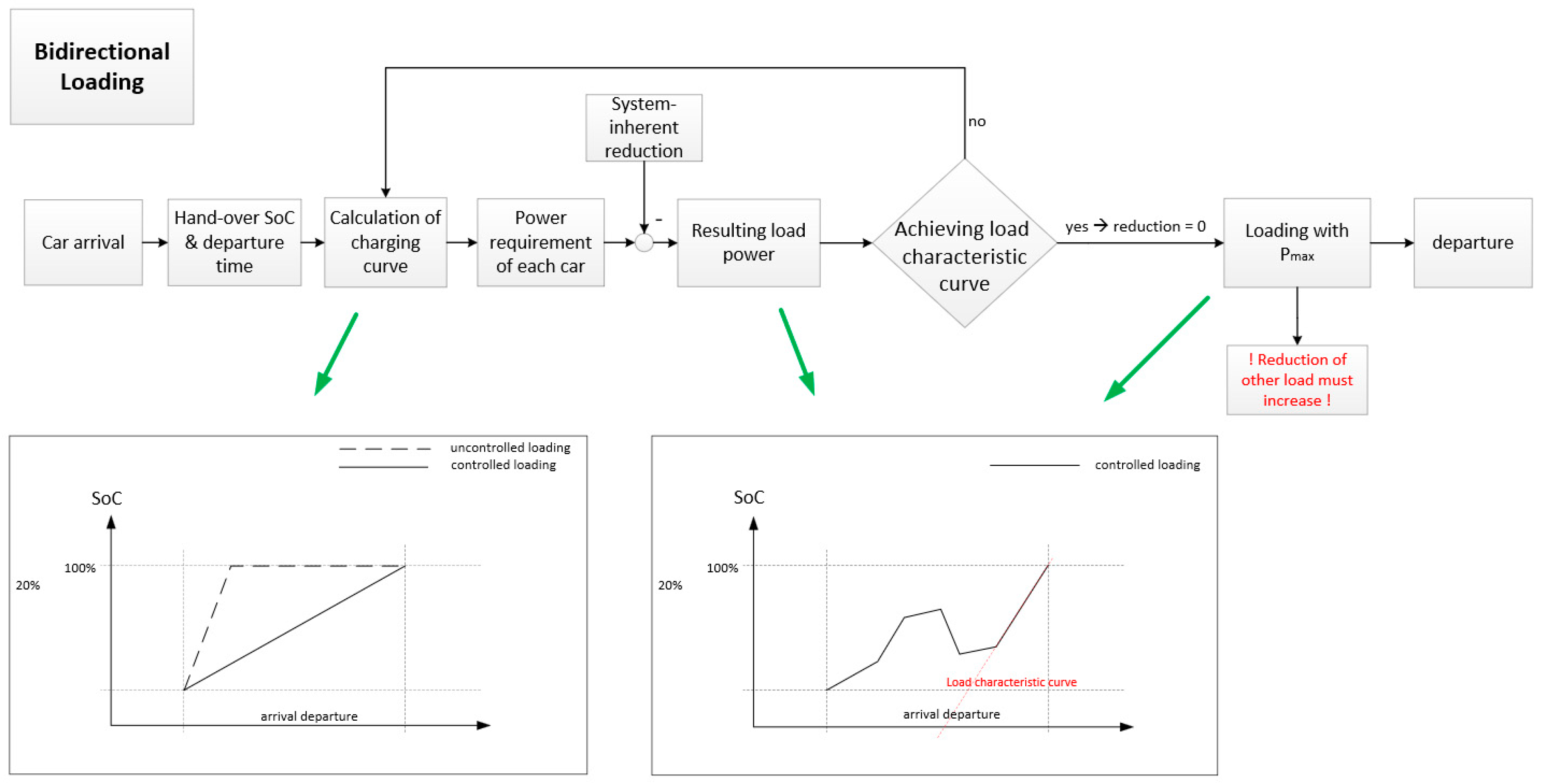
Upon arrival of the electric vehicle at the charging station, the current state of charge (SoC) and the maximum loading capacity of the car will be automatically transferred to the control system. Furthermore, the user of the car is required to communicate his/her most probable departure time via a user interface. From this information, the charging characteristic is calculated for the car to be loaded during the service time. Depending on the system, it may be advantageous if the car is loaded according to different charge characteristics, e.g., at lunchtime, the grid load should be minimized.

After calculating the charge curve, the car has a defined power requirement. This power requirement cannot be always provided due to lack of power or energy from the superimposed system. Therefore, the system calculates for each car a coefficient of attenuation that controls the power consumption of the car. From the departure time, initial SoC and the maximum load capacity of the car, its characteristic curve can be calculated, so that the battery achieves planned SoC for the specified departure time point.

If an additional parameter for the minimum SoC (<100%) is set for the departure time by the user, it increases the degree of freedom for the timing of maximum power charging. However, a minimal residual SoC should be always guaranteed to allow unexpected trips and emergency driving. If the characteristic curve is reached, the load attenuation is ignored, and the car is loaded with maximum power. This additional power requirement must be provided by attenuation of all other loads (or some selected loads) in the system. If this is not possible for technical reasons, the car at the departure time cannot be fully charged.

The following functional block diagram in Figure 1 shows the load behavior of a bi-directional electric car with the possibility of limiting the charge power by the host system.

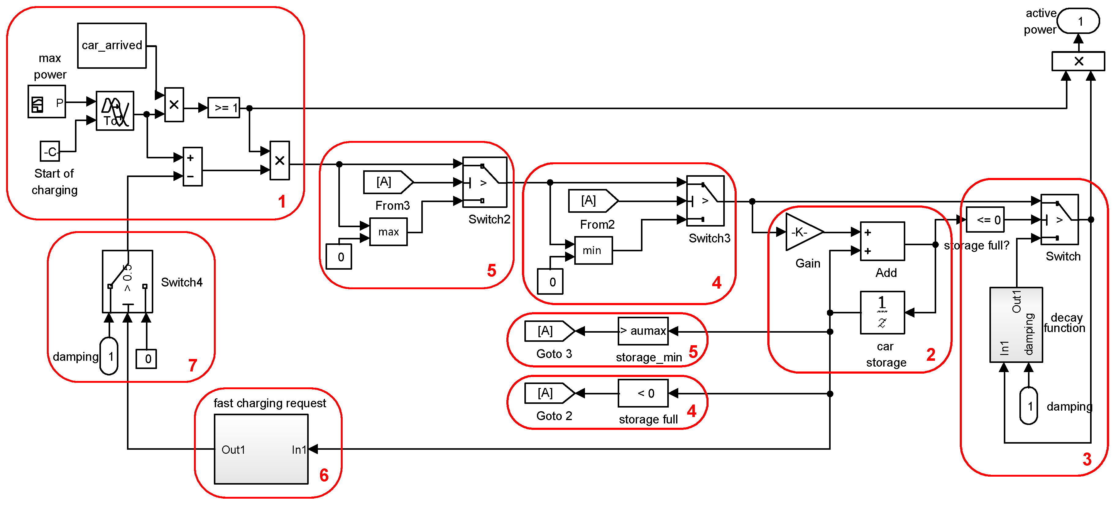
Example of a Controllable Load in Simulink

The following shows an implementation of controllable load. For clarity, only the active power is considered, since it is not presentable to include the reactive power in the model. The reactive power generation is however analogous to the active power generation. Figure 2 shows a screenshot of the Simulink model. For clarity, the model is divided into seven sections (red boxes), and subsections will be discussed separately below. The following paragraphs correspond to the order of the numbered boxes.

(1)

A binary block (0/1) tells if the electric vehicle is active during the day and performs initialization (car_arrived). A signal builder generates for the charging time of the car (here determined as the average of the field test data) the maximal charge in uncontrolled load mode. Power consumption is delayed to the arrival time at the charging station.

(2)

The initialization state of charge of the car (determined as the averaged value from field tests) will be loaded with the power value generated by the signal builder until the battery is fully charged. The exact value of the charge depends on the technology of the battery. In the absence of empirical data, a value of 99% can be assumed.

(3)

When the SoC threshold is achieved, the power consumption goes into a decay curve until eventually the battery is completely loaded. If the battery is fully charged, the system goes into trickle charge. This was in the field determined with 0.2 kW, but is heavily dependent on the particular system.

(4)

If the battery is fully charged before the departure time (set by the user) is reached, no more energy can be fed into the battery; however, the battery can still be discharged into the system, if allowed by other constraints.

(5)

The battery can be discharged to supply the system only until a minimum value is reached (to be defined by the user). Subsequently, only positive values can be transferred to the battery module.

(6)

As described previously, the charging characteristic must define when limiting of the charging power becomes ineffective, so that the battery at departure has the desired SoC.

(7)

The limit is determined from the available system power. If the available power of the microgrid is lower than the needs of all electric vehicles, all are limited to the extent that the power balance is reached. The limitation of charging power can be enforced uniformly. All active vehicles are limitable in the system that are not fully discharged or excluded by reaching the boundary of the charging characteristic. The individual limitation of electric cars requires high computing power and would cause the simulation to be unnecessarily complicated.

5.2. Modeling of Feature-Dependent Generation

Feature-dependent generation, as PV systems, means by their variability strong challenges to the secure network operation. Renewable energy sources may be disconnected only as a last resort to maintain the safe operation of the grid, according to widely-adopted grid codes. In the simulation, the calculation step must be set to less than one second to reflect the strong variability of infeed by PV systems. The loss of information about the system dynamics is at longer simulation steps not tolerable and leads to unacceptable errors [18].

Within a microgrid, the PV infeed must be cut down by the control system if the supply exceeds the load and the available storage is fully charged. Furthermore, there may be an important power surplus if the PV system is oversized. Again, appropriate action must be taken in the course of the supply-dependent feed. To record the loss by depression of the PV output, a separate measuring device is required, recording the history of the irradiation. Such a measuring device can consist of one or more measuring cells that are locally installed close to the PV system. Evidence that a PV system can be simulated accurately by a simple measuring device is shown [19]. It was demonstrated that a PV system with various geographical orientations of panels can be mapped by a few cells with acceptable error. 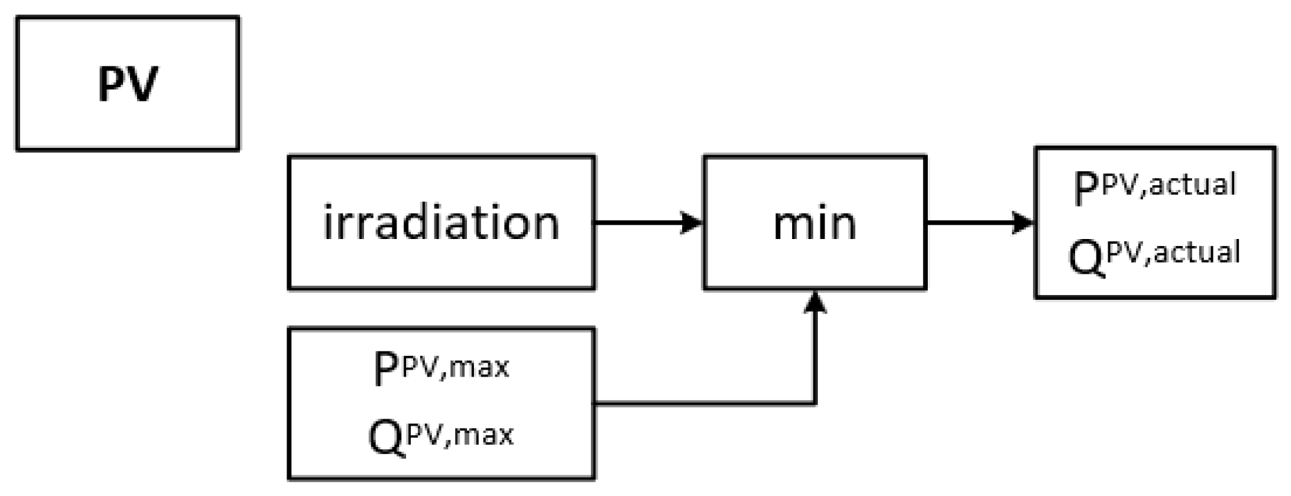Figure 3 shows the flowchart of the PV-irradiation model in a microgrid. P_PV,max and Q_PV,max represent the maximum possible feed, required at a given time point by the microgrid. Current infeed will have always a lower value (power generated from the current PV insolation or the maximum required power by the microgrid).

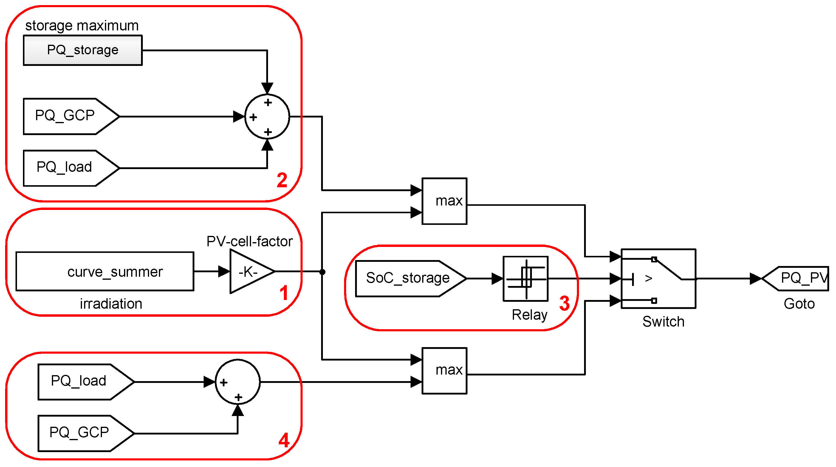
Example of PV Infeed Modelling in Simulink

The following shows an example implementation of the PV supply system. Figure 4 shows a screenshot of the Simulink model. For clarity, the model is divided into four sections (red boxes). The following paragraphs correspond to the order according to the numbering of boxes.

Through the block “From file”, the irradiation values are input to the simulation. Here, it is important to pay attention to the correct sign of the input values (for the used consumer power meter, negative values for active power are provided to the control system). By the factor K is set the size the PV system and efficiency. It is recommended not to set the direction and angle of the PV plant over a factor K in the simulation, but to do it beforehand in the irradiation values’ calculation. The factor K can be adjusted during an optimization. If no measured value series to define the PV infeed are available, the historical data from available databases can be used alternatively. However, doing so will cause loss of the real gradients of irradiation.

(1)

For the power balance within the closed unit of a microgrid, the radiation must be limited to the power requirements of the elements of the microgrid. For this purpose, the maximum power feed to the storage, real-time power requirement of the load, as well as the real-time power requirement superimposed grid are added together. This represents the upper limit of power consumption in the microgrid. The correct sign is assured via the matcher “min/max”, so the power in the system does not exceed the limit. From the comparison between the input values and system set values, the possible PV irradiation limitation can be determined. This comparison has not been realized in the model shown, since it can be determined (if desired) directly from the simulation system.

(2)

The limit on the PV infeed described in 2 must be adjusted as soon as the existing system storage cannot absorb more energy. For this, the SoC of the storage has to be incorporated into the PV model over a “From” block. Via a relay, the real-time SoC of storage is compared with a definable value. When achieved, the switch block is switched to the second path. In order to prevent an infinite loop in the circuit of the switch block (when the state of the storage corresponds to the limit value and with the switching, the level drops, this forces the repeated switching), a second threshold value may be set in the relay; for that, the relay is to be only switched again. For the upper limit, a value less than 100% should be selected since the microgrid elements may show a time constant, so although the switching command has been issued, the response is delayed (SoC recommendation = 99%). The lower threshold should have a distance of less than 2% of the SoC to prevent unnecessary PV limitations (SoC recommendation = 98%).

(3)

If the limit of the SoC is reached, the power cannot be fed into the system, resulting from the real-time power requirement of the load and the real-time power demand from the grid. This summed power demand corresponds to the maximum power that is fed into the system.

In this model, the size and the efficiency of the PV system is set and the infeed by the PV system is regulated by the observation of the SoC of the storage. The comparison of the possible and the actual PV output is determined by the simulation. Other provisions of the infeed regulation are not necessary.

5.3. Modeling of Controllable Generation

Controllable feeds (feature-independent feeds) supply the system with power on the desired schedule or in response to a demand for support coming from the control system. A variant of controllable feeds represents current-controlled CHPs.

From the standby state, the micro-CHP must be synchronized once to the grid after the start command issued by the control system. After this synchronization, the CHP unit can be adjusted to the desired infeed. The time constant for the change from one state to another depends on the device. The heat production (if included in the simulation) can be passed to the heat storage, if available in the system. The heat storage unit represents a limitation to the mini-CHP. When heat storage is full, the mini-CHP unit must be shut down.

In a simulation, the current-controlled mini-(micro-)CHP can be viewed as a simple infeed that can provide full power at any time. The distinction between active and reactive power is important, as both powers can be provided independently and have different minimums and maximums. Reactive power can be provided as capacitive or inductive.

Reaction times when changing between the set values of the active power can be estimated with a maximum of 5 s, as long as no measurements or the manufacturer’s data are available. Reactive power can be assumed to change step-wise. For network synchronization, a time constant of less than 30 s can be assumed. The thermal power of the mini-CHP is in direct reference to the electric power. If the manufacturer’s data are not given, the ratio of 1:2 can as first approximation be assumed (double heat output for the electric power output). With this ratio, a rough estimate can be made whether an existing size of storage is sufficient. In [20], the ratio of 1:1 for future current-controlled CHP is proposed. If the storage is completely full, the mini-CHP unit cannot be operated if no other heat dissipation in the system is available. Where the micro-CHP is connected to the district heating network, the heat production can be neglected and heat storage assumed to be infinite.

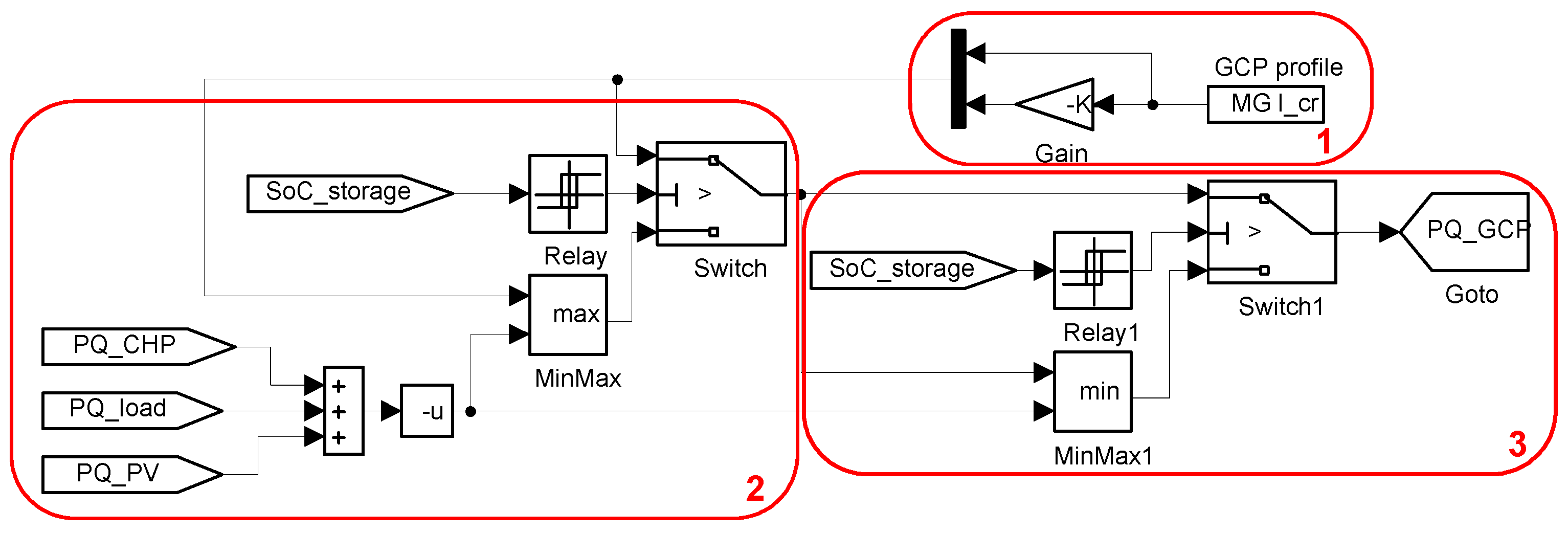
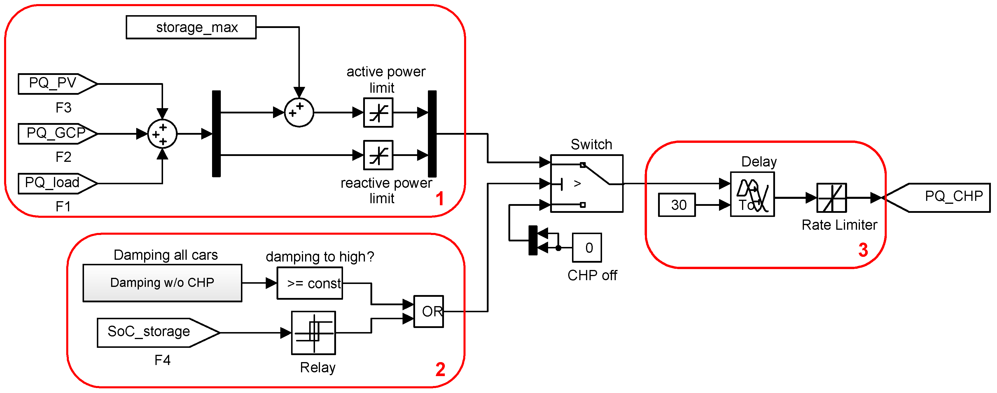
Example of CHP Modelling in Simulink

In the following, an exemplary implementation of the mini-CHP can be carried out in Simulink. Figure 5 shows a screenshot of the Simulink model.

(1)

In order to determine the active and reactive power required by the system, the real-time power values of the active components are added. Only real power is to be made available to the storage from the mini-CHP. The minimum (=0), as well as the maximum (>0) are limited for the active power by means of a “saturation” block. The maximum can be set by a variable during the initialization, which was defined in the workspace. As a result, the power of the mini-CHP can be easily adapted during optimization. The reactive power has independent limits of the real power, so a separate “saturation block” is necessary.

(2)

A logical “OR” operator is used to decide under which conditions the mini-CHP is required. On the one hand, the mini-CHP is switched on when the storage level falls below a defined SoC (e.g., 10%). Then, the mini-CHP remains switched on until the storage reaches a second threshold value (e.g., 50%). On the other hand, the mini-CHP is used as support to charge the electric cars. When limiting the charging power per car (50% of the maximum power), the mini-CHP is also switched on until the load limitation of the load drops below this value.

(3)

A “delay” block and a “rate limiter” block are used for the reaction time and the rate of change of the mini-CHP. The respective values can be taken from the manufacturers’ data.

5.4. Modelling of Storage

In a microgrid, like in any other electric power system, generation and consumption must be tuned permanently to each other. If the production is based mainly or partly on feature-dependent sources (see Section 5.2), the balancing of these sources by a storage systems can take place. An overview of storage technologies according to their energy transformation type is described in [21]. The work in [22] shows an overview of storage technologies categorized by discharging times in relation to the rated power.

Depending on the objectives, the appropriate storage technology can be determined for the planned microgrid. Electrochemical storage (batteries) is suitable as stationary storage within microgrids by its technical maturity, market availability and reliability.

The power required by the system is retrieved from storage to its technical limits. Since batteries are connected via the inverter to the microgrid, it can be assumed that there are no delays between the load demand and infeed from the storage.

In modeling, a storage has four key parameters: active power, reactive power, actual energy content and state of charge (SoC). The storage as the reactive element in the system can provide energy to the system and absorb energy to its maximum load. Between these limits, the delivery and uptake must be limited, because of the technical limitations of inverters.

For the calculation of the energy balance, the physical effects (such as voltage dips) can be neglected. However, the maximum depth of discharge must be defined for a value, where such effects are negligible. Since the recommended discharge state for, e.g., lead-acid batteries is 70%, to increase number of life cycles, voltage-related data do not play a decisive role in the simulation. Voltage-related considerations, however, are included in the evaluation of the required storage size, as in the simulation, only the amount of available energy can be incorporated, but not the installed energy.

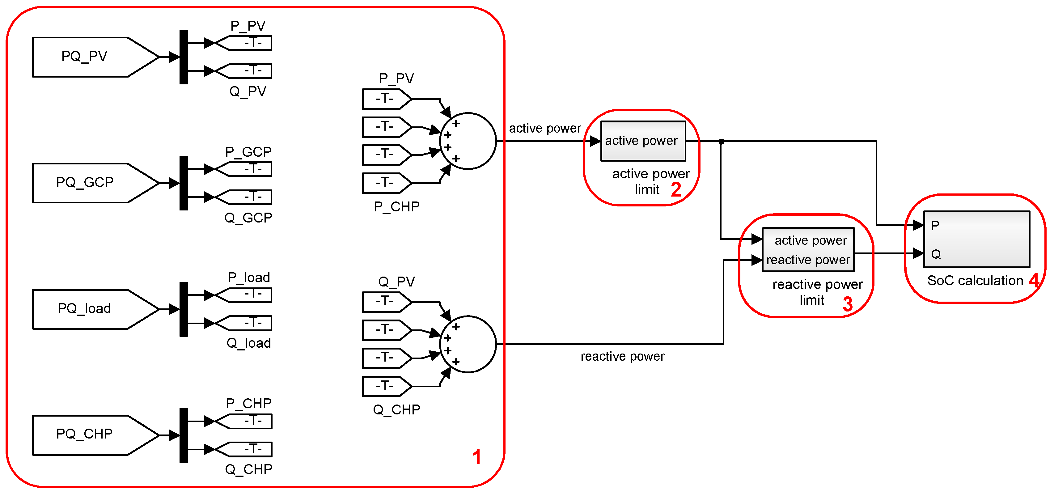
Example of Storage Modelling

An exemplary storage simulation implementation in Simulink is shown in Figure 6.

(1)

The real power and reactive power of all elements of the microgrid are combined. For this purpose, the instantaneous active and power performance values of all models are imported into the model storage via a “From” block and are then added separately according to active and reactive power.

(2)

Since the real power of the storage is limited, the sum of the active power of all other components must be limited to the minimum and maximum. For this purpose, an upper and lower limit value can be entered. Since all components have their own limitations, which is based on the maximum of the storage, there should be in principle no violation of the limit values. In order to be able to calculate the actual storage from the simulation, however, the limit value violations, should they occur, should be included in the simulation. For example, a limit value may be briefly exceeded if an electric car is connected to a charging column. These excesses can be realized by short-term overloading of the inverter of the storage.

(3)

For clarity, the simple reactive power limitation and SoC determination are omitted.

6. Interconnection of Components within the Microgrid

In general, the three classes of components, supply, storage and load, are interconnected and connected to the superimposed power grid. Any component may be connected and fed directly into any other component. The energy of the storage can be fed to both the load and the host network, and from the superimposed grid, in turn, the charging of the storage is possible. Furthermore, the load can be fed directly from the host network. From this general fully-interconnected model, a specific model can be derived, required for the simulation of the real microgrid. It is also necessary to incorporate technical or regulatory constraints that may limit the flow of energy. For example, an infeed from the energy storage into the superimposed power grid must be suppressed, because the feed from the storage is not considered a renewable-source energy by the regulations. If the feed from the storage cannot be separately measured, it must be technically prevented.

7. Modelling of the Power Grid

In order to be able to estimate the possibilities of a microgrid operation mode, it is necessary to determine which task a microgrid should take over within the energy transmission network. The infeed of energy from the microgrid into the superimposed power network at high load times, as well as the uptake of energy in weak load times represents a meaningful task and can be used for basic considerations. The residual load at the network connection point of the selected medium voltage network to the high voltage network is the reference load profile. In order to visualize this load profile, the medium voltage network to be investigated must be simulated with all loads and feeders for a dynamic load calculation. If the medium-voltage network is not known or only insufficiently known, various medium-voltage benchmark networks can be used. Figure 7 shows the medium-voltage benchmark network of International Council for Large Electric Systems (CIGRE) with 30 nodes [23].

The outputs of nodes Kn00 to Kn29 represent loads for which the standard load profiles can be set if no real load profiles of the grid to be examined are available. With this modeled grid, a dynamic load flow calculation can be carried out, resulting in the load profile of the overall network. Capacity bottlenecks in the power supply network are neglected. If, however, the power supply network is sufficiently known, the integration of these real load profiles at the designated location must be taken into account in the generation of the load curves for the microgrid. The microgrid can be connected in parallel to the grid, so the microgrid only affects the load. Figure 8 shows the basic connection point in the benchmark network shown above (a partial view was chosen for clarity).

The CIGRE benchmark network was simulated for the transfer profile at the grid connection point, and the standard load profiles were set at the network nodes. Figure 9 shows the simulated load profile for a weekday, Saturday and Sunday for the winter, transition and summer seasons.

Modelling of a Grid Connection Point

An exemplary implementation of the network connection point can be carried out in Simulink. Figure 10 shows a screenshot of the model.

(1)

The load profile (Figure 9) is loaded into the model via a “from file” block. We assume a constant power factor over the entire simulation time of the model. The reactive power curve can be determined accordingly.

(2)

If the storage can take up the energy from the grid connection point, the power that is to be fed into the microgrid from the network can be assumed without restriction. According to these specifications, the storage must be designed in such a way that the power flow is positive, as well as negative. If the storage is full, only the power that is needed as the balance of the other microgrid elements can enter into the system.

(3)

This also applies to the power that the microgrid can provide to the superimposed network. Here, as long as the storage has enough energy, an unrestricted availability can be assumed. However, if the storage is empty, only the balance of power of the other components can be assumed as available.

8. Optimization of Microgrid Components

Microgrids are suitable for achieving certain goals. Common to all of these goals is that the components are designed to meet the requirements of the microgrid and must be dimensioned in their critical properties. In order not to oversize the components, which adversely affects the profitability of a microgrid, the optimal component sizes have to be found [24]. In order to properly dimension the components within the microgrid, an optimization is required. For nonlinear problems with constraints, found here, the trust-region optimization presents a suitable method [25].

The trust region is a term used in mathematical optimization to denote the subset of the region of the objective function that is approximated using a model function (often a quadratic). If an adequate model of the objective function is found within the trust region, then the region is expanded; conversely, if the approximation is poor, then the region is contracted. The fit is evaluated by comparing the ratio of expected improvement from the model approximation with the actual improvement observed in the objective function. A model function is “trusted” only in the region where it provides a reasonable approximation. For clarity, we do not provide more details on this optimization method. The theoretical and practical implementation aspects can be found, e.g., in [26,27].

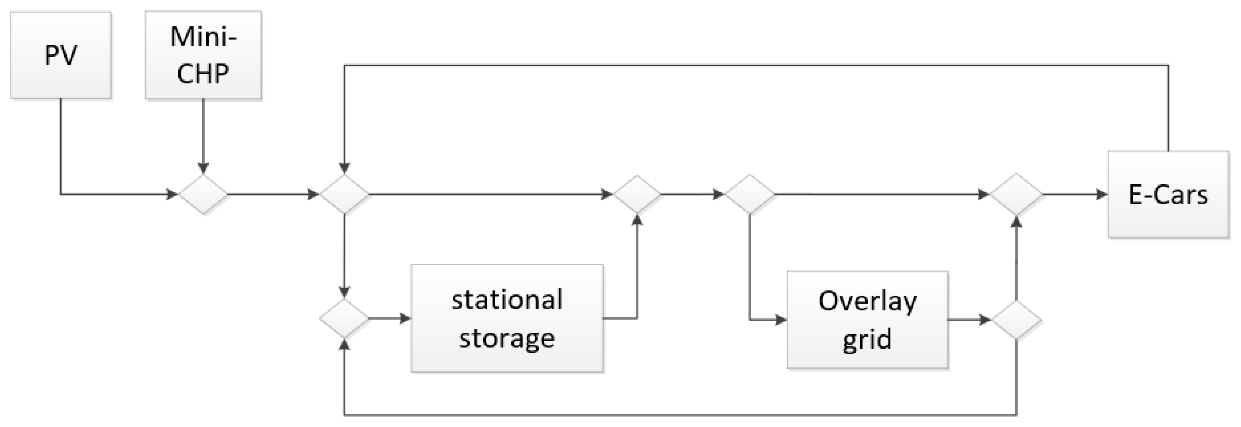
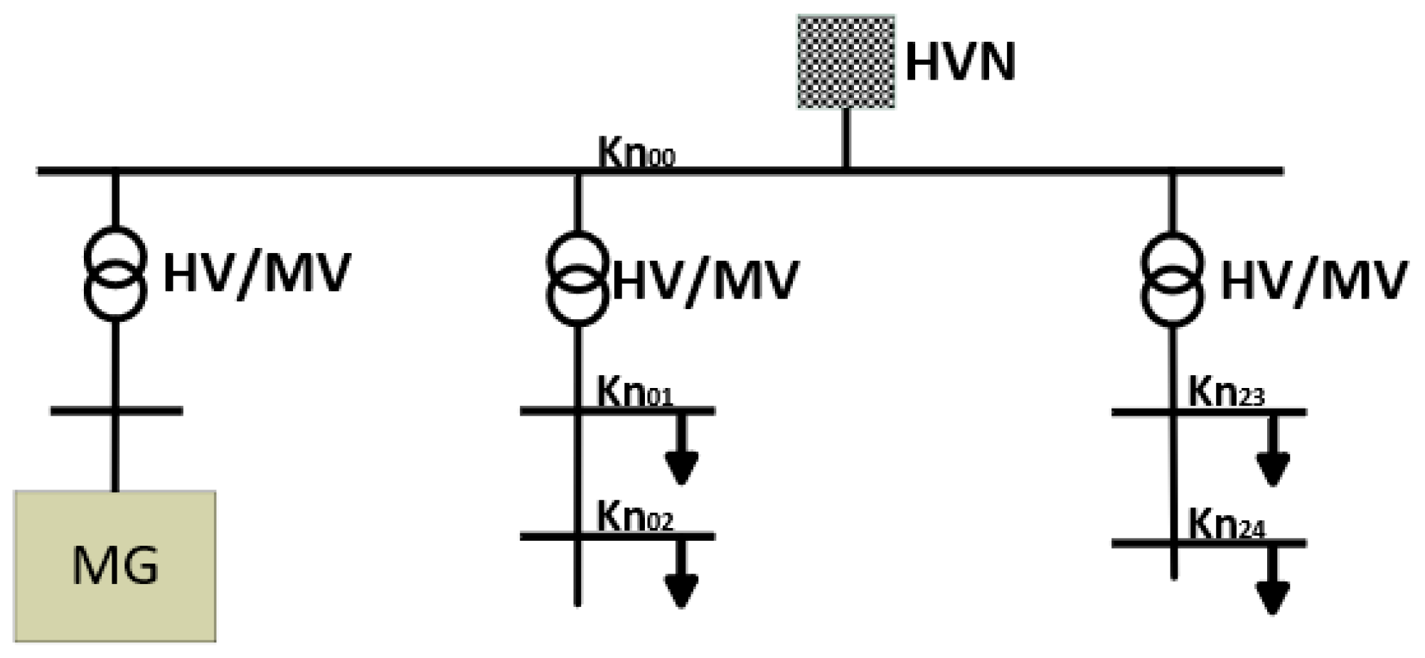
Figure 11 shows the energy flow of a sample plant where a PV plant and a mini-CHP are used as feeders, a stationary battery as energy storage, electric cars currently shown exclusively as a controllable load and to be eventually considered later as bidirectional units, as well as a superimposed medium voltage network.

The bi-directionality is considered, although currently, it is not sufficiently scientifically documented regarding the influence, limits and possibilities of bidirectional electric cars on the superimposed energy network, in this case the microgrid. In case of such an interconnection for the simulation of a real microgrid, it must be ensured that there may be technical or regulatory limiting conditions that can restrict the flow of energy.

In the example shown, as well as in the other chapters, it is assumed that no regulatory restrictions are to be observed. The control of each component, including the regenerative supply, as well as the supply to or from the superimposed power supply network is possible. For bidirectional controllable electric cars, it is assumed that the energy flow from the load into the storage, as well as into the superimposed power supply network is possible. Technical limitations such as capacity bottlenecks of the technical network components (power cables, transformers, etc.) are not taken into consideration, as the simulations as presented here are energy balancing models.

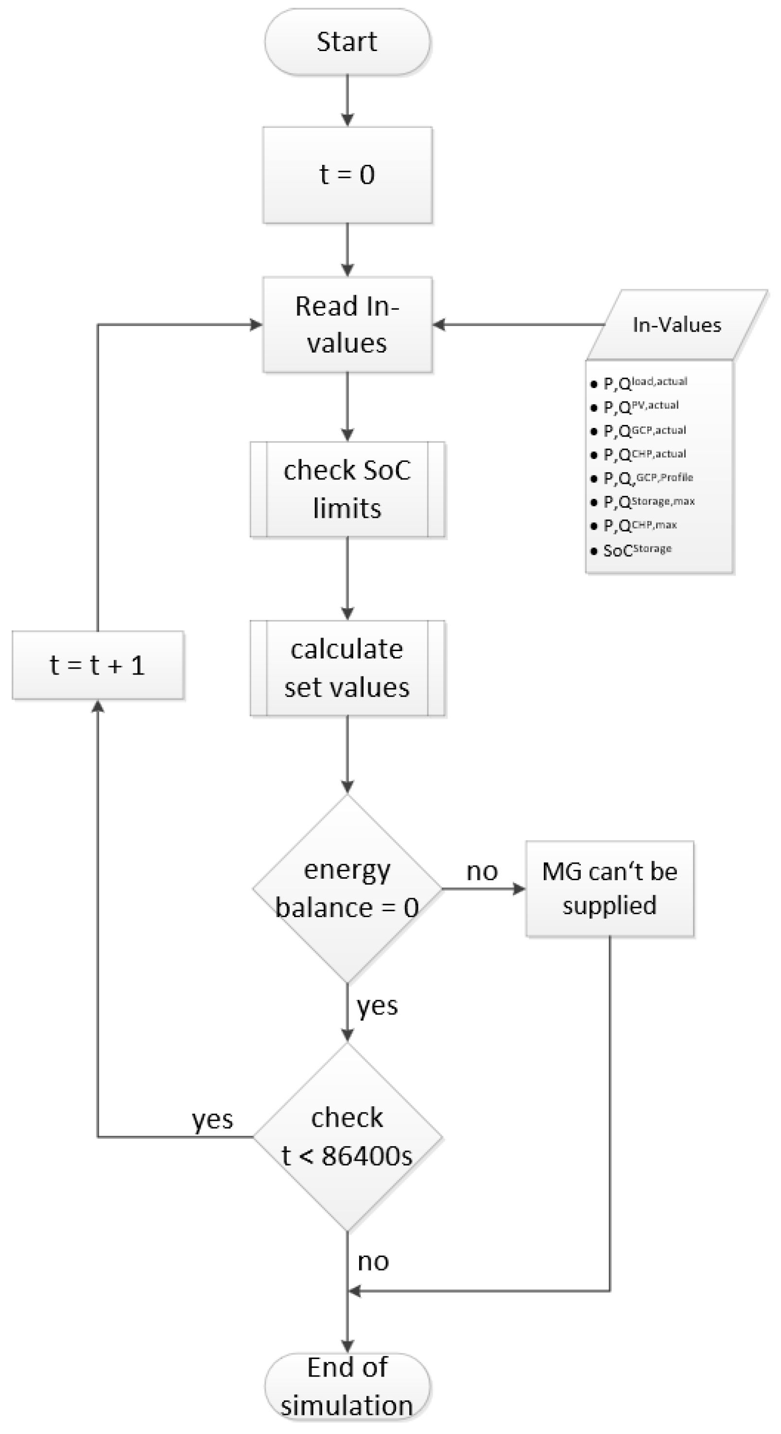
A possible sequence of the simulation of a microgrid is shown in Figure 12. Here, a 24-h simulation is described as an example with a one-second simulation step. At the beginning of the simulation (starting at time t = 0), the initial values of all components of the model are read. The initial values include the states (for example, the mini-CHP is in standby, the charge state of the storage, the number of the controllable loads, etc.), as well as the values for the active and reactive power. These values can then be used to check whether all limit values are complied with.

If the end of the duration to be simulated has been reached (here 24 h) and the energy balance has been equalized, the simulation is terminated successfully. For reasons of clarity, the flow chart shown in Figure 12 does not show whether the simulation targets have been met. The unconditional supply of the load is not taken into account in this flowchart, for example, and requires further algorithms, which must be used to check all simulation-specific targets. These algorithms can be implemented during the limit value check or the modeling of the components themselves, leading to a simulation termination or a subsequent message after the simulation has been completed. A simulation-oriented goal can be, for example, the complete supply of the load, the maximum use of the PV energy or the compliance with the prescribed curves on the grid connection point. A combination of all objectives is also conceivable. Targets can either be initialized directly in the simulation as a termination criterion (for example, when the PV generation was limited, even though full use is desired) or evaluated after the simulation. It is therefore left to the programmer.

The limit-value check is an integral part of the simulation of a microgrid. In a simulation step, the limit values entered by the user are compared with the actual values occurring in the simulation at this time step. If the limits are not met, measures are formulated for the next simulation step. In the configuration shown here, the state of charge state (SoC) of the stationary storage is the leading quantity. If set charging states are exceeded, measures are taken for the next simulation step. If, for example, the limit value has fallen below (here, SoC < 20%), the mini-CHP is started as an additional supply. When the lowest limit is reached, the entire microgrid load profile is subjected to a limitation.

8.1. Control Concepts for Microgrids with a Focus on the Load Supply

The premise for each control concept of a public or semi-public microgrid must be the relief of the upstream network while at the same time meeting all network requirements within the microgrid, as well as the complete load supply, the latter having a very high-ranking role. A microgrid control concept, in which the load supply is not top priority, is theoretically conceivable, but will lead to a strong rejection by the users of the electric vehicles in a real implementation.

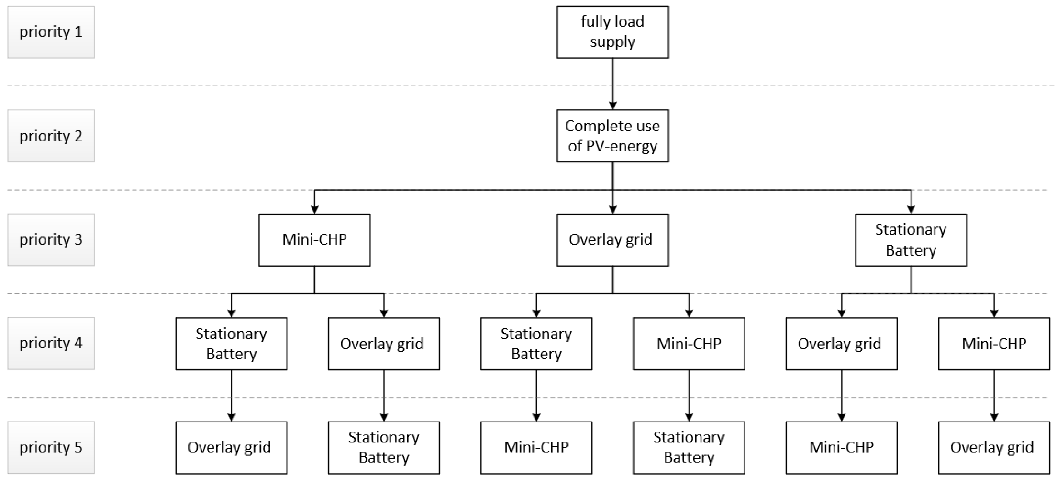
Using a priority tree, the variety of possibilities for prioritization can be demonstrated. A priority tree with five components [16] shows 120 options for the priority order of the components. Taking into account the unconditional load supply and the subsequent use of all available PV energy, the reasonable possibilities are reduced to six, which are shown in a tree structure in Figure 13. The control system in a complex system, such as a microgrid model, can either be defined by one of the components themselves or implemented separately by a superimposed controller.

The stationary storage is suitable as a guide component. If, on the other hand, circular references occur between the components, that is if mutually-dependent components refer to one another, they are unsuitable as a control-guiding component. A circular cover occurs in a microgrid between supply and load. The load can only supply as much power in a closed system as the supply is currently available. The feed-in components, on the other hand, can feed only as much into the system as the load allows. This circular dependence has the effect of an infinite loop in a simulation when the PV system or the load is selected as the guide component.

This circular dependence between the PV system and the load can be broken by implementing a component that represents the maximum possible irradiation through the simulated PV system. Thus, the load can serve as a guide variable for the PV system while the load adjusts to the maximum possible power that is to a separated component. This separate component then represents, for example, a measuring device that has been placed locally close to the PV system and with the aid of which, the available irradiation is transmitted to the system. If the SoC of the stationary storage is selected as the guide variable, care must be taken of the delays of the components’ reaction during the control. For example, a mini-CHP has a certain initial and post-run time, so that the system can react immediately, but the desired effect is delayed. A limit value for the system reaction must be selected with a safety buffer, so that the battery is not charged above 100% or discharged to less than 0%. In order to be able to depict these effects adequately, a simulation in the millisecond clock is required. Exceeding the limit values can result in large inaccuracies during longer cycle times, as a result of which, information loss may occur when limiting the values. A two-point control should always be used for a limit implementation. Such a two-point control prevents an oscillation between two states when a limit value overshoot leads to a reaction, which would prevent the limit value from being exceeded. A two-point control has a dead region corresponding to a hysteresis. In this way, for example, the mini-CHP can be connected if the stationary storage falls below a defined SoC and is only switched off again when a higher SoC is reached. The mini-CHP will then be switched off again until the lower limit value is reached. Such regulations should be implemented for all supply and related components to ensure system stability.

8.2. Optimization of Microgrid to Support a Medium Voltage Network

The example is of a microgrid with 10 electric cars supplied by a PV system, a storage unit and a mini-CHP unit, while at the same time, a load profile on the grid connection point is to be maintained. By optimizing the component sizing, the smallest possible setup of the photovoltaic system, the mini-CHP and the storage battery can be found, which can be used to supply both the load and the specified load profile at the GCP without having to down-regulate the PV system. The control algorithms and limit values are set according to the example of Figure 12, unless otherwise mentioned in the component description. The storage has an SoC of 5% at initialization of the model and is used to temporarily store the PV energy, as well as to ensure the load profile. The cars are only loaded from the storage when they go into quick charge mode and the power within the microgrid is not sufficient. This microgrid model corresponds to an industrial microgrid as described in Section 4.3.

8.2.1. Feature-Dependent Generation

The solar irradiance values in a German city were recorded with a measuring instrument for a complete year for the supply-dependent feed. The measuring instrument consists of 33 measuring cells arranged on a spherical surface. As shown in [19], such a measuring instrument can be used to perform an almost exact reproduction of each photovoltaic system in the immediate vicinity of the measuring device. From the measured values, an average curve for each cell was created separately for the period of summer. From a combination of different cells, a representative curve can be created for any PV plant. From all curves measured in the summer period (orientation south, angle of inclination 45°), an average curve is formed, which represents the average single-beam values for this period. These injection values are introduced into the simulation. The starting value is an installed power of the photovoltaic system of 80 kW peak, which is to be viewed as an optimization variable.

8.2.2. Storage

The storage technology is insignificant for the simulation since no transient effects, such as voltage dips, etc., are considered. The stationary storage is modeled with an initial apparent power of 60 kVA and an initial capacity of 200 kWh, where apparent power and capacity represent the two variables to be optimized. The capacity calculated in the simulation represents the usable energy of the required storage and, depending on the storage technology, must be transferred according to the energy to be installed. Since the relationship between usable and installed energy differs greatly depending on the technology, the transfer is not used at this point.

8.2.3. Load

Ten bi-directional electric cars for the simulation are modeled according to the procedure described in Section 5.1. The average time of arrival and the average service life of each car were determined from the field tests carried out by electric car drivers. For the arrival time, a random value is calculated for each day in the determined time span. The average absorbed energy was calculated from the measurement data of the first three of four test periods (18 months in total).

The required energy per car is 9–20 kWh (total of 169 kWh). Again, the values of the test drivers measured in the field test were used. The maximum required power per car is 9.5 kW. Each electric car can be controlled up to a minimum power of minus 9.5 kW, so that it is possible to feed the energy back from the car storage to the microgrid. Here, the state of charge of each car is considered separately. Until the time of departure, each car must be fully charged.

When the electric car is fully charged, only the power required to maintain the charge is drawn from the system until the user or the superimposed system disconnects the electric car from the charging column. Between arrival and departure, the electric car can be freely controlled within the simulation until the charging curve is reached. The load is assumed to be constant, i.e., all electric cars are simulated with corresponding power and corresponding energy requirements. They are not varied during optimization.

8.2.4. Mini-CHP

The mini-CHP modeled as in Section 5.3 is activated in the simulation if the stationary storage falls below a critical value of 5% or the load is limited by more than 50% of the maximum power. When a load condition of 20% or a reduced load limit is reached, the mini-CHP is switched off, taking into account the start-up and stopping times. The heat component of the mini-CHP is neglected as it is assumed that the mini-CHP is connected to the heating network, so that this heating network is an infinite heat storage from the point of view of the mini-CHP. The mini-CHP is inserted into the simulation as a starting value with a power of 0 kVA. Later, it is added in increments of 5 kVA separately to illustrate the relationships between the increase in the power of the mini-CHP and the reduction in the performance of the other feeding components.

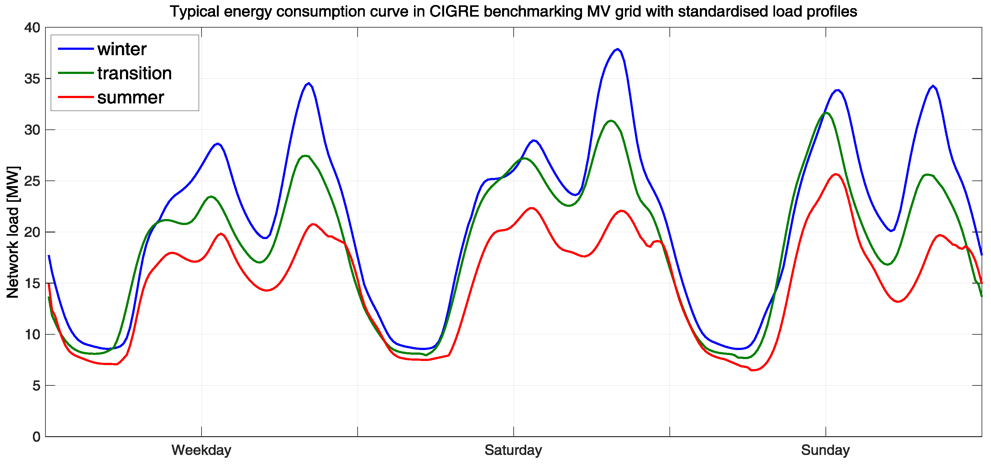
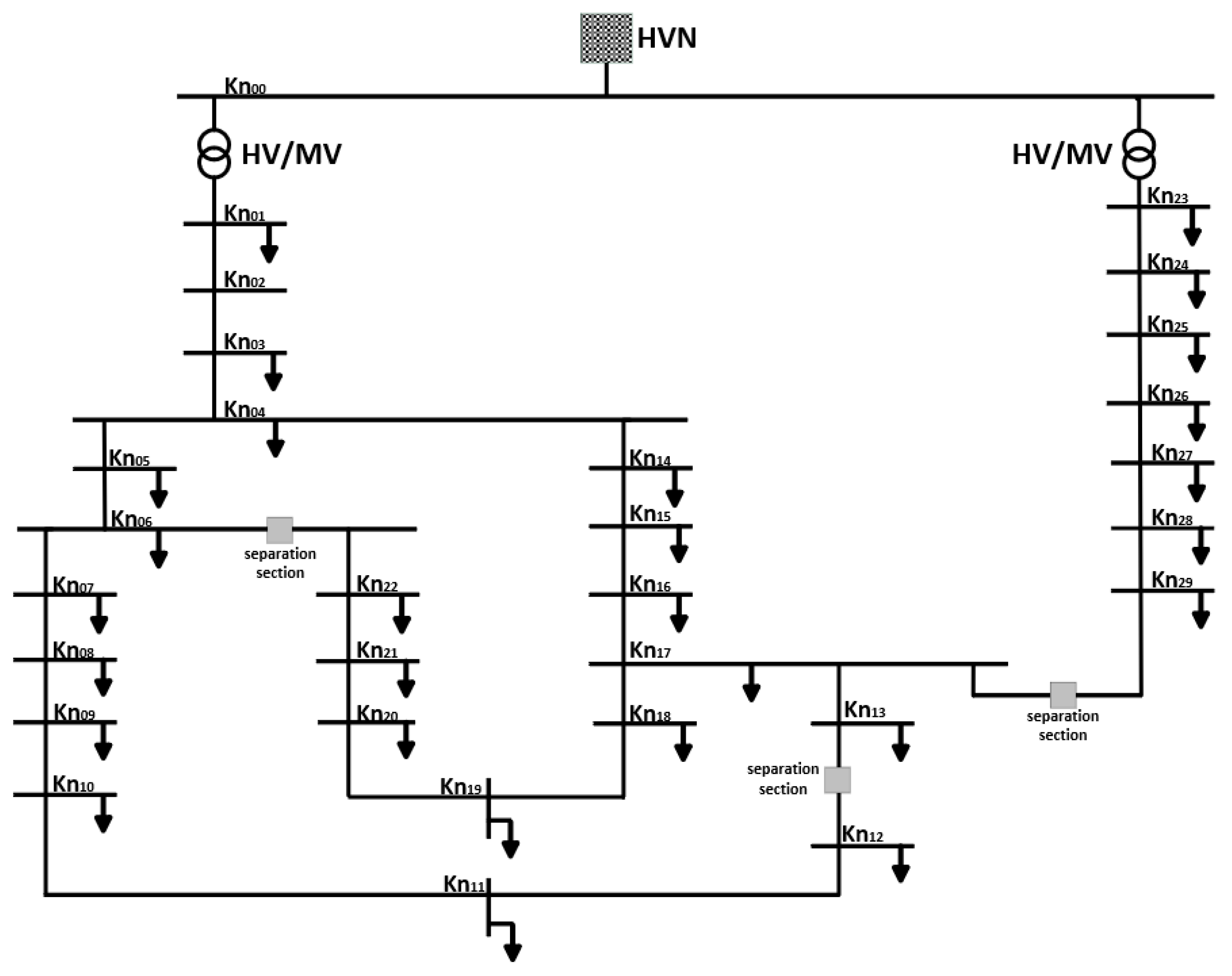
The CIGRE benchmark network, as described in Section 7 was simulated for the transfer profile at the GCP, and the standard load profiles were set at the network nodes.

8.3. Optimization of Components

With the help of the optimization procedure presented in Section 8, the components of a PV system, storage and mini-CHP are to be chosen in such a way that all conditions are fulfilled:

(1)

All electric cars are fully charged at the end of the day,

(2)

No PV energy has been lost and

(3)

The default load profile has been fully followed at the GCP.

The target function is:

$$F\left(w,x,y,z\right)=\parallel P_{\mathrm{GCP},\mathrm{set}}-P_{\mathrm{GCP},\mathrm{sim}}{\left(w,x,y,z\right)\parallel }_2-\parallel P_{\mathrm{PV},\mathrm{set}}-P_{\mathrm{PV},\mathrm{sim}}{\left(w,x,y,z\right)\parallel }_2$$

(1)

where $w$ is storage power, $x$ is storage energy, $y$ is power of the PV system, $z$ is power of the mini-CHP unit, $P_{\mathrm{GCP},\mathrm{set}}$ = default GPC load profile, $P_{\mathrm{GCP},\mathrm{sim}}$ simulated GPC load, $P_{\mathrm{PV},\mathrm{set}}$ input-PV power, from irradiation and $P_{\mathrm{PV},\mathrm{sim}}$ simulated PV power.

8.4. Results of Optimization and Discussion

In order to find a suitable starting point for the optimization, the energy balance within the microgrid is considered over a whole day. For this purpose, the required daily energy quantity of the cars (111 kWh) and the daily energy amount at the GCP (180 kWh) are added with correct signs. The amount of energy required must be provided by the PV system and the mini-CHP unit. Neglecting the mini-CHP, the above-described PV system has an installed power of 74 kW for an average summer day. This configuration makes it possible to determine the storage capacity of 100 kWh and a storage power of 26 kW. Figure 14 shows the real-time load profiles of the GCP, the PV system and the electric cars in kW, as well as the percentage of consumption in the load for the defined component dimensioning.

It becomes clear that with the chosen storage dimensioning, the energy of the PV system can be shifted in time so that no energy is lost. When the electric cars arrive, the energy available in the microgrid is not enough to charge the electric cars. It is even necessary to extract energy from the electric cars for the microgrid in order to be able to meet the default profile at the GCP. The energy flow changes as soon as enough energy is available through the PV system or from the superimposed power grid. At the end of the usage period of the electric cars, these were fully charged without violating the predefined profile at the GCP. The next step is to introduce the mini-CHP in the range from 0 kW–30 kW in 5 kW steps in the simulation. All other components within the microgrid are not changed any further. For reasons of clarity, the representation of the performance profiles of all calculated variants is omitted.

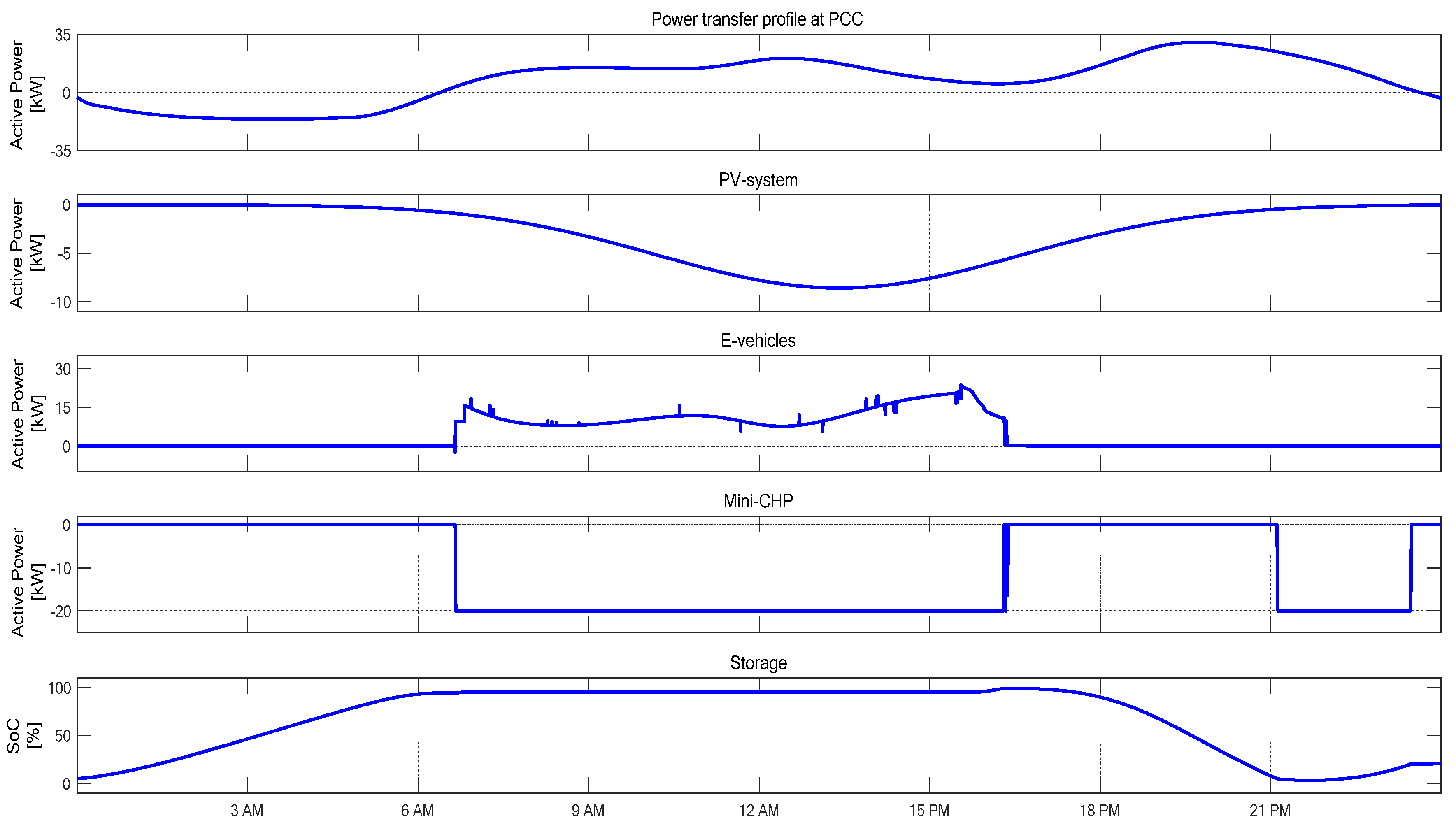
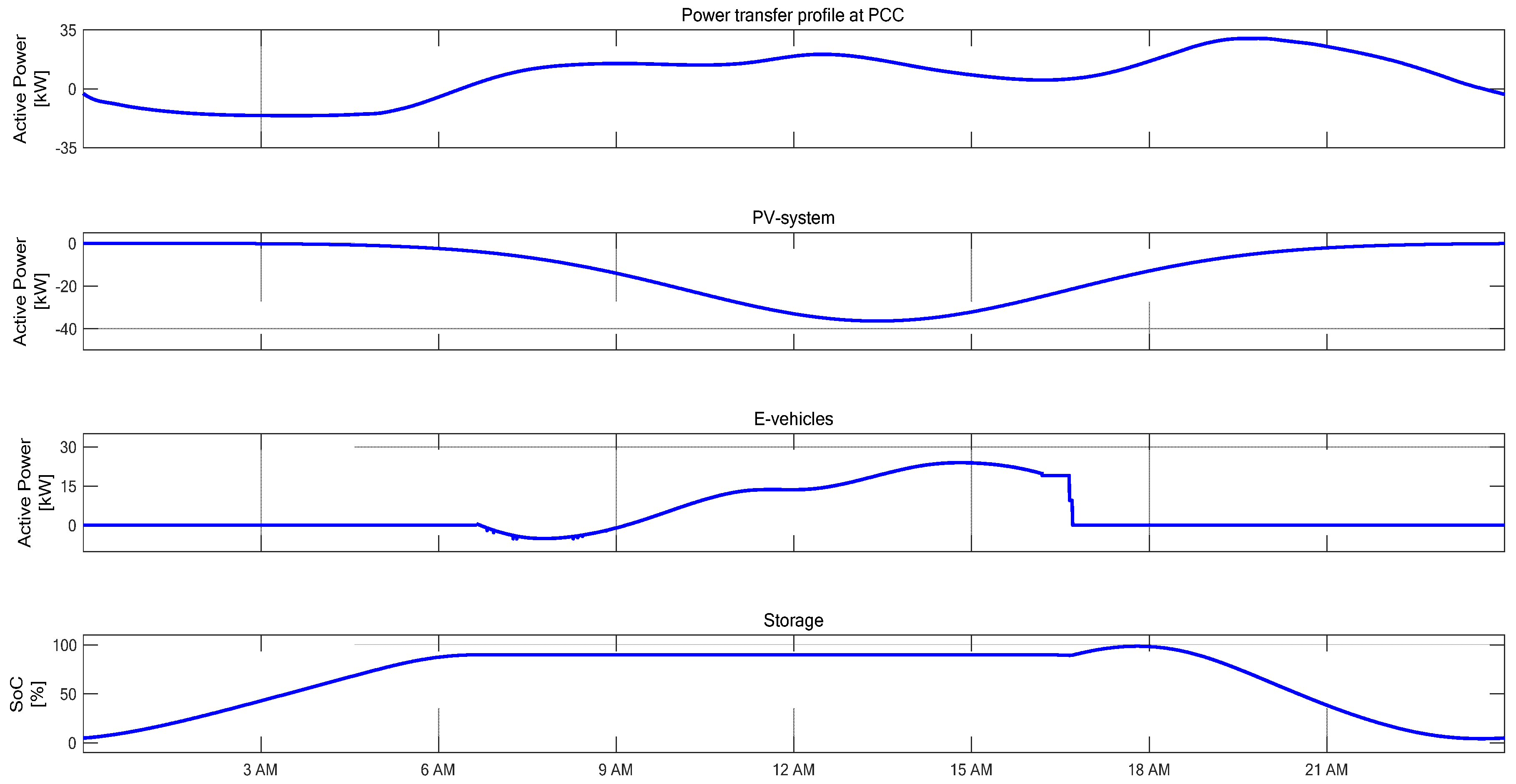
Figure 15 shows the performance curves for the variant with a mini-CHP of 20 kW. The mini-CHP is used to support the charging of the electric cars until the charge is no longer limited to more than 50% (see the mini-CHP model) or the electric cars are fully charged. Furthermore, it supports compliance with the specified transfer profile at the GCP, when the energy in the storage is no longer sufficient.

Due to the simulated control characteristics, the mini-CHP recharges the storage again if enough power is available. This behavior is programmed in the algorithm and can be modified so that the mini-CHP is only used to support the charging of the electric cars and to assure the compliance of the GCP load profile so that the storage would not be charged.

Table 1. Results of the optimization of the component storage and PV as a function of the selected mini-CHP power.

Mini-CHP	PV	Storage Capacity	Storage Power
0 kW	74 kW	100 kWh	26 kW
5 kW	61 kW	100 kWh	26 kW
10 kW	49 kW	96 kWh	26 kW
15 kW	35 kW	91 kWh	26 kW
20 kW	18 kW	91 kWh	26 kW
25 kW	10 kW	91 kWh	26 kW
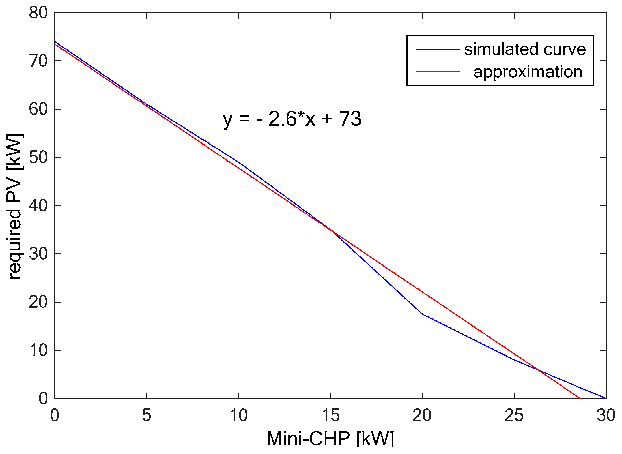
30 kW	0 kW	91 kWh	26 kW

shows the results of the optimization for the component storage and PV as a function of the selected mini-CHP power parameter. As can be clearly seen, there is almost no relation between the mini-CHP and the storage in the example shown. The storage dimensioning takes place predominantly on the basis of the predefined load profile at the GCP, specifically due to the uptake of energy from the superimposed network into the microgrid before the electric cars are connected. There is, however, a clear relation between the required PV power and the dimensioning of the mini-CHP. If the required PV power is plotted above the installed mini-CHP power, a straight line can be approximated by a simple curve fitting, which is given by the function $f\left(x\right)=2.6x+73$.

Figure 16 shows this relationship graphically. From this diagram, it is also possible to estimate the power required for a mini-CHP so that the power within the microgrid is still sufficient on low-radiation days. Since, in the summer, a large range of different solar radiations can be covered by installing a mini-CHP, the microgrid’s objectives can still be achieved.

9. Discussion and Outlook

Although there are relations between the feed-in components for a component dimensioning, no direct relationship between the storage dimensioning and the dimensioning of the PV system or the mini-CHP could be established. The feed-in components complement each other linearly so that the available power within the microgrid can be assumed to be constant. The storage is used to vary the energy over time so that it can be assumed that the required capacity does not change with the power within the microgrid. For the sizing of the battery, the energy absorbed from the superimposed energy network is primarily decisive in the example presented here. Furthermore, it was found that the objectives of the microgrid to be defined beforehand, as well as the objectives of each component strongly affect the dimensioning. A change in the control characteristics leads directly to an adaptation of the required component dimensions and must therefore be determined before the component optimization, or be treated as an optimization variable, in order to adapt the required components to their own objectives.

In this paper, microgrids were generally described and classified. The diversity of the component composition and the importance of the dimensioning of each individual component for the corresponding application area were demonstrated. It was shown how optimization of component sizing is possible. For this purpose, an example microgrid is simulated. It has been found that component sizing is strongly dependent on the objectives and the target algorithm to be defined.

A change in the control algorithm for a component requires the re-dimensioning of all components to be considered within the microgrid.

Further studies have shown that the nine variants resulting from the summer, winter and transition seasons and the three working days of the week, Saturday and Sunday, lead to different dimensions of the required components despite the same goals and the unchanged algorithm. Therefore, all nine variants should be simulated and the components separately optimized in order to be able to define a variant that corresponds to the desired goals.

Beyond the example microgrid shown here, the heat component is a very important factor. Especially in the winter, a mini-CHP is predominantly controlled to cover the heat demand. The dimensioning of the mini-CHP is thus dependent on the control variable (current controlled or heat controlled). Thus, after a separate dimensioning of the mini-CHP due to the heat requirement, this can enter into the optimization as a fixed variable so that the mini-CHP is not further adapted during the component dimensioning of the microgrid. The dimensioning of the required components within a microgrid is possible so that an over-dimensioning and thus an extension of the economic payback time can be prevented.