Model-Based Predictive Current Control Method with Constant Switching Frequency for Single-Phase Voltage Source Inverters

Abstract

Voltage source inverters operated by predictive control methods generally lead to a variable switching frequency, because predictive control methods generate switching operation based on an optimal voltage state selected at every sampling period. Varying switching frequencies make it difficult to design output filters of voltage source inverters. This paper proposes a predictive control algorithm with a constant switching frequency for the load current control of single-phase voltage source inverters. This method selects two future optimal voltage states used in the subsequent sampling period, which are a zero-voltage state and a future optimal voltage state, based on the slope of the reference current at each sampling period. After selecting the two future voltages, the proposed method distributes them to produce a constant switching frequency and symmetric switching pattern. The performance of the proposed method is validated with both simulation and experimental results for single-phase voltage source inverters.

1. Introduction

With the increasing popularity of renewable energy systems, single-phase converters for grid-connected systems with distributed power generation sources, such as those for photovoltaic (PV) panels [1], electric vehicles [2], and railway systems [3], have been used more often for relatively low-power applications. One of the main objectives of single-phase converters and inverters is to synthesize a high-quality ac-side sinusoidal current tracking a reference current, to transfer the power required by a variety of systems. For generating a sinusoidal line or load current with low harmonic distortion, control methods for the single-phase converters or inverters usually handle the ac-side sinusoidal current [4,5,6,7,8,9]. The current control methods, based on proportional-integral (PI) controllers, in [4], have been generally utilized; however, steady-state current errors exist in the ac-side current because of exposure of the PI controller to low-frequency fundamental components. In addition to the PI-controller-based current control methods to eliminate the steady-state error, numerous approaches have been proposed to reduce current errors, such as hysteresis control [5], deadbeat control [6], proportional-resonant (PR) control [7], voltage-oriented control [8], and predictive control [9]. In particular, the predictive control method has been widely used to control the ac-side current of single-phase converters [10], inverters [11], and other topologies [12,13] as a simple and effective technique due to the development of digital signal processors with low cost and high performance [14,15,16]. The predictive control method for ac-side current control predicts future current movements by using system models. On the basis of predicting control variables, the method directly selects an optimal switching state to be applied to the next step in such a way as to minimize the control errors, described in terms of a cost function criterion, without producing switching patterns by pulse width modulation (PWM) blocks. The predictive control method can lead to such merits as fast transient behaviors and a simple structure lacking dedicated modulation blocks. On the other hand, one of the disadvantages of the predictive control method is a varying switching frequency, because the switching pattern depends on the optimal switching state decided arbitrarily by the cost function at each control period. The variable switching frequency and correspondingly spread frequency spectrum with numerous harmonic components in the converter voltage and current waveforms result in difficulty in designing the output filter. Furthermore, a single application of an optimal switching state during the entire switching period can lead to large ripple components in the output current waveforms. Therefore, there have been several studies on converter operations with a constant switching frequency based on the platform of predictive control methods. Several techniques have been developed for the predictive control methods with constant switching frequency for three-phase inverters and converters [17,18,19,20,21,22]. Ref. [17] proposed the direct power control (DPC) for a three-phase voltage source converter. In this method, an optimal vector was selected using the model-based reference voltage in the αβ stationary coordinate frame, and the duty cycle and vector distribution were determined by the conventional space vector pulse width modulation (SVPWM). Ref. [18] proposed the direct torque control (DTC) for permanent magnet synchronous motor (PMSM) drive, where an optimal reference voltage and the angle were calculated for vector selection through the cost function. In addition, the duty cycle and the vector distribution were obtained using the conventional SVPWM to obtain a constant switching frequency. Ref. [19] selects an optimal vector using the model-based reference voltage in the synchronous dq coordinate frame and uses the conventional SVPWM to decide the duty cycle and vector placement. Ref. [20] proposed the predictive current control (PCC) for the three-phase converters used in wind turbine, where optimal vectors are selected using the angles of the grid voltages and the optimal duty cycle is calculated by differentiating the cost function. This method also uses SVPWM to obtain a constant switching frequency. Ref. [21] proposed a DTC for PMSM motor drive. In order to obtain the constant switching frequency, the vector was selected using the model-based reference voltage in the stationary coordinate frame same as Ref. [17], and the duty cycle and vector placement were determined using the conventional SVPWM. Ref. [22] uses the grid voltage angle to select the vector and calculate the duty cycle at which the power error is zero in the next step. Moreover, SVPWM is used to obtain a constant switching frequency in this method. All the approaches for the three phase converters [17,18,19,20,21,22] use the pulse width modulation (PWM) blocks, for generating a fixed switching frequency based on the predictive control method.

Studies to achieve a constant switching frequency in the platform of the predictive control for single-phase converters have less revealed than those for the three phase converters [10,23]. Both approaches for predictive power control construct a virtual two-phase system from single-phase signals and employ pulsewidth modulation blocks. Ref. [10] creates two virtual phases using the angle of the input source voltage to extend single phase axis to stationary αβ axes for generating the optimal αβ reference voltage vector. Based on the resultant optimal reference voltage vector, a space vector pulsewidth modulation (PWM) block is used to switching patterns with constant switching frequency. Similar approach was addressed in Ref. [23], which develops the model predictive direct power control with constant switching frequency. In this paper, fictitious orthogonal phase voltages and currents are generated from a single-phase quantity by a second-order generalized integrator. Using the generated virtual quantities, an optimal modulation index for predictive power control is calculated and is passed through a carrier-based PWM generator.

This paper proposes an improved predictive current control method with a fixed switching frequency for single-phase voltage source inverters, without employing PWM blocks. On the contrast to the conventional approaches for the single-phase converters, the proposed method selects the optimal voltage states using only the slope of the reference current. This approach is simpler because the optimal switching state can be easily selected without constructing the virtual orthogonal quantities, in comparison with the existing studies of the single-phase converters. In addition, the proposed method develops switching patterns with a fixed switching frequency by appropriately dividing the zero-voltage state and the non-zero-voltage state, without employing the PWM modules. Thus, the proposed method can create a constant switching frequency based on the predictive control method with simple control structure and algorithm, in comparison with the previous approaches. The harmonic spectrum of output currents and voltages obtained by the proposed predictive control method are concentrated on multiple switching-frequency regions, without output harmonic components spread over wide frequency ranges. With the proposed scheme, the centralized harmonics of the output current and the voltage with fixed switching frequency, which can help to design output filters, are obtained without employing a PWM block. Simulation and experimental results for both the steady-state and dynamic responses are provided to demonstrate the effectiveness of the proposed method. The proposed predictive current control method is compared with a conventional predictive current control method and a carrier-based PWM method with a PI current controller, where the fast Fourier transform (FFT) analysis of the proposed method reveals similar switching patterns achieved by a carrier-based PWM method with a PI current controller.

2. Conventional Predictive Current Control Method for Single-Phase Voltage Source Converters

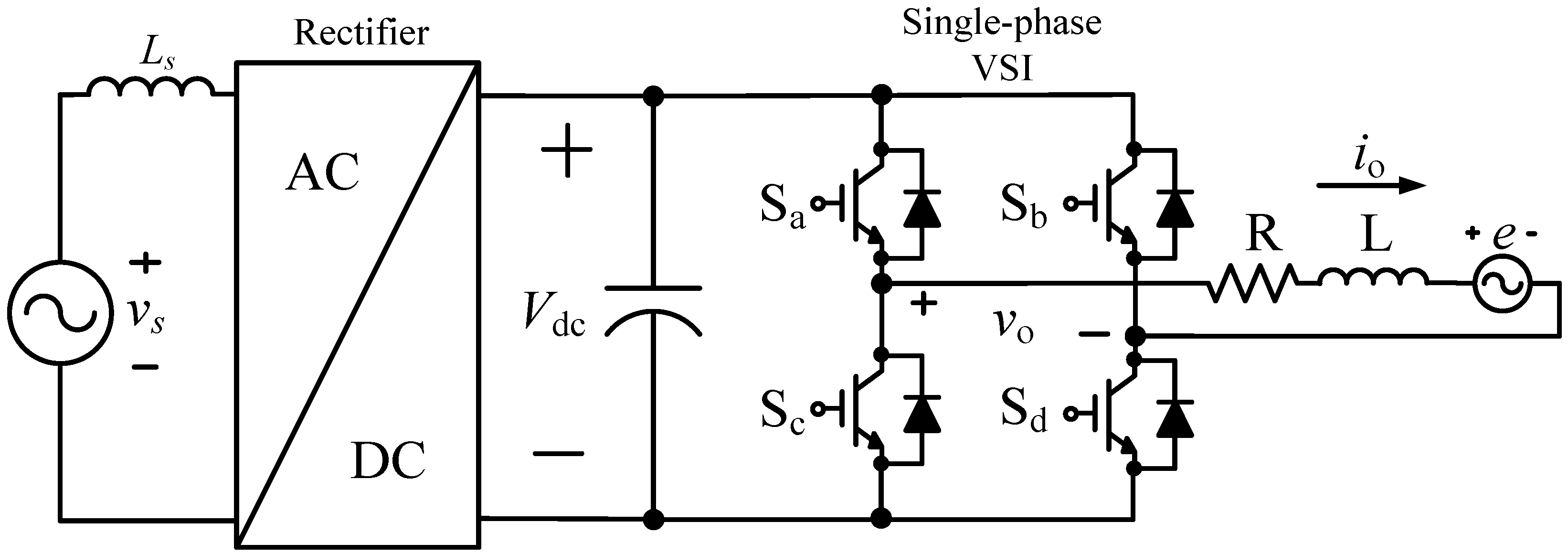
Figure 1 shows a single-phase voltage source inverter that consists of a general resistive-inductive load and back-electromotive force (back-emf) with four switch components as well as a diode rectifier. The conventional model predictive control (MPC) method [24], which is called the conv-MPC method in this paper, for a single-phase inverter can employ one optimal voltage, which leads the possibly smallest current error at every sampling instant. In the single-phase inverter, there are three individual output voltages which can only make three different current behaviors to loads connected to the converter. Thus, the relationship of the output voltage (v_o(t)) and current (i_o(t)) in Figure 1 is given by

$$v_o\left(t\right)=R{i}_o\left(t\right)+L\frac{d{i}_o\left(t\right)}{dt}+e\left(t\right),$$

(1)

where R, L, and e(t) are the load resistance, inductance, and back-electromotive force (back-emf), respectively. On the basis of the sampling period [$n{T}_s$, $(n+1)T_s$], (1) can be written in discrete form as:

$$i_o[(n+1)T_s]=i_o[n{T}_s]+\frac{T_s}{L}(v_o[n{T}_s]-R{i}_o[n{T}_s]-e[n{T}_s]).$$

(2)

where i_o[nT_s], v_o[nT_s], and e[nT_s] are load current, load voltage, and back-electromotive force (back-emf) at the present step, respectively.

Moreover, the present back-emf needed in (2) can be assumed to be equal to the back-emf one step prior because the sampling frequency is much faster than the frequency of the back-emf voltage as

$$e[n{T}_s]\approx \widehat{e}[(n-1)T_s]=\left(v_o[(n-1)T_s]-R{i}_o[(n-1)T_s]\right)-\frac{L}{T_s}\left[i_o\left[n{T}_s\right]-i_o[(n-1)T_s]\right].$$

(3)

With the output current dynamics presented in (2), three future current acts made by three output voltages can be predicted for the single-phase inverter. The optimal voltage is selected among three voltages used for the single-phase inverter, which reduces current errors between the next-step actual load current (i_o[(n + 1)T_s]) and the reference current (i_o*[(n + 1)T_s]) by estimating the output current dynamics at every sampling period. The cost function to judge the current error can be described by the future current error between the reference current and the predicted current as

$$g=\left|i_o^{*}[(n+1)T_s]-i_o[(n+1)T_s]\right|.$$

(4)

The above future reference current needed for the cost function is acquired in the Lagrange extrapolation, with the past and present reference values, by [25]

$$i_o^{*}\left[\right(n+1)T_s]=3i_o^{*}\left[\right(n+1)T_s]-3i_o^{*}\left[\right(n-1)T_s]+i_o^{*}\left[\right(n-2)T_s].$$

(5)

where i_o*[nT_s], i_o*[(n − 1)T_s], and i_o*[(n − 2)T_s] are the reference load current at the present-step, the one-step before, and the two-step before, respectively.

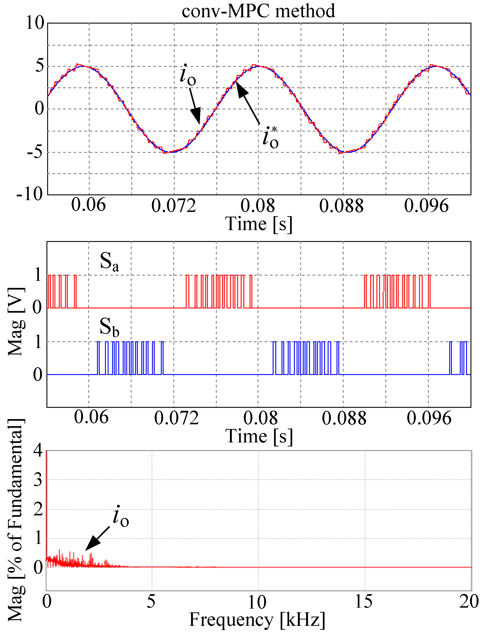
A simulation waveform of the output current of the single-phase inverter obtained by the conv-MPC method is shown in Figure 2. The switching pattern waveforms and the fast Fourier transform (FFT) waveform are also included in Figure 2, where the frequency spectrum was spread over a wide range of frequencies.

3. Proposed Predictive Control Method for Single-Phase Inverter

In the proposed method addressed in this paper, two voltages, among the three achievable in the single-phase voltage source inverter (VSI), are selected and applied in one sampling period, which affects switching patterns with a constant switching frequency, such as those of sinusoidal PWM (SPWM) combined with the PI controller [26]. After choosing the two voltages, the two selected voltages are adequately divided to synthesize the switching forms with a fixed switching frequency. There exist three sets with two voltages in the single-phase VSI, which are {0, V_dc}, {0, −V_dc}, and {−V_dc, V_dc}. However, a set with {V_dc, −V_dc} obviously leads to the largest current ripples in the output current. Thus, the proposed method incorporates the advantages of two sets with two voltages, i.e., {0, V_dc} and {0, −V_dc}.

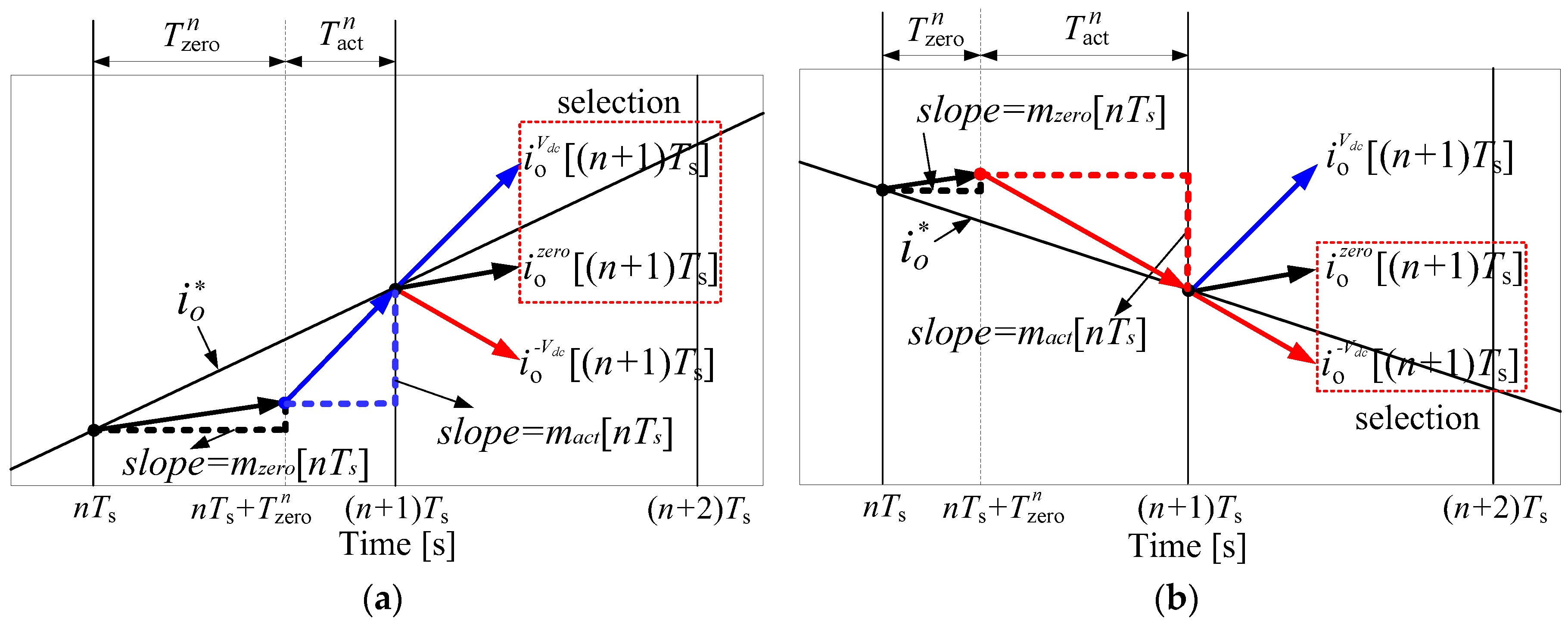
Figure 3 shows the concept of the proposed method with the two sets of two voltages, e.g., {0, V_dc} and {0, −V_dc}, where the proposed method is forced to a no-current error at every sampling instant. It is seen that one set between the two sets can be simply selected on the basis of reference current slope. As shown in Figure 3, the load current created by applying the voltage V_dc in Equation (2) is represented by $i_o^{V_{dc}}[(n+2)T_s]$. Similarly, the load currents created by applying zero and −V_dc voltage are denoted $i_o^{zero}[(n+2)T_s]$ and $i_o^{{-V}_{dc}}[(n+2)T_s]$, respectively. As shown in Figure 3a, in the case in which the reference current at the next step is higher than the reference at the present step, the set {0, V_dc} is used to increase the actual current in the next step. On the other hand, a set {0, −V_dc} is applied to decrease the actual current when the slope of the reference current is negative, as shown in Figure 3b.

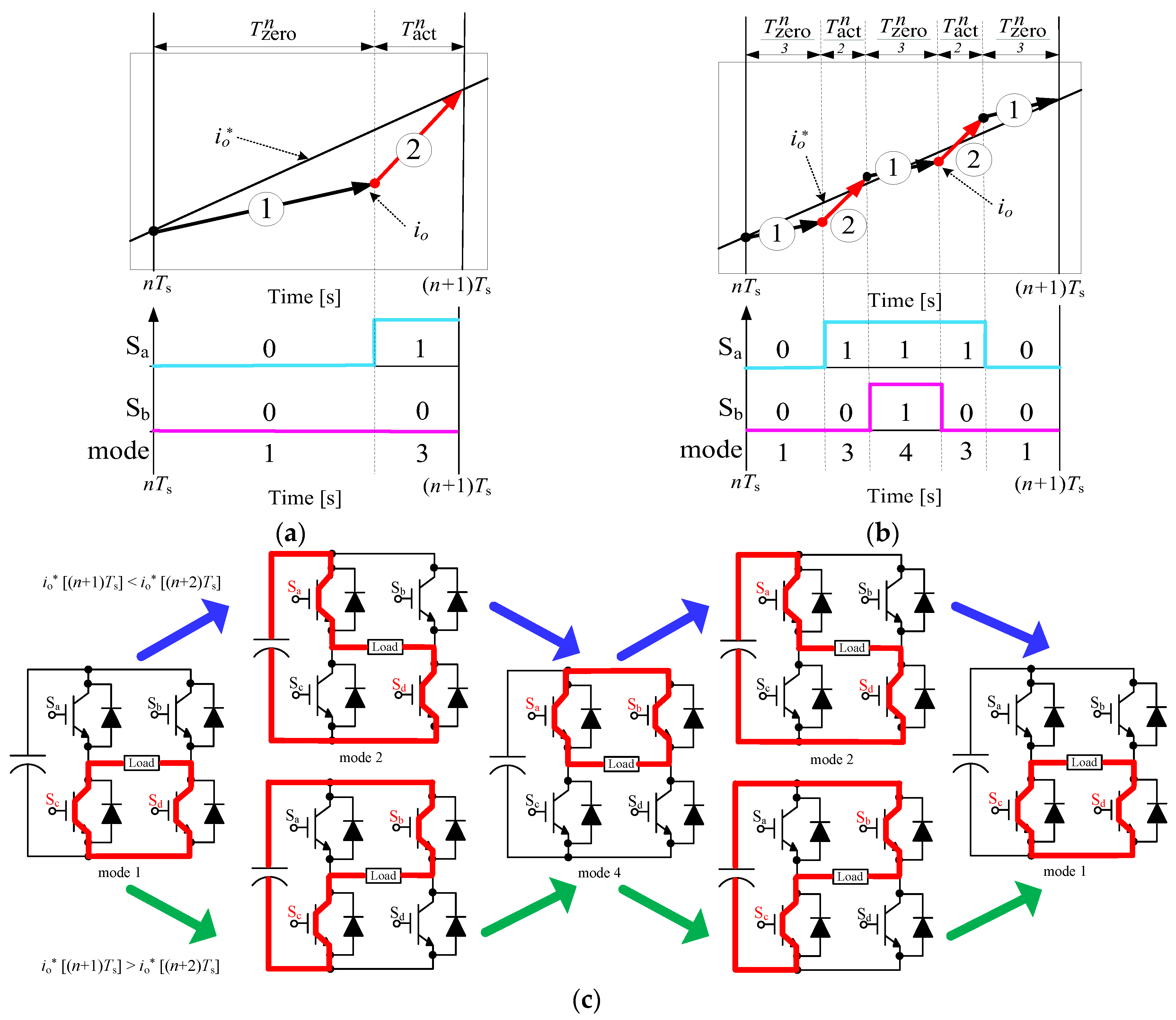
Assume that $T_{zero}^n$ and $T_{act}^n$ are the time durations for the zero-voltage and the active voltage, such as V_dc and −V_dc, in the nth sampling period, respectively. In one sampling period T_s, it always should be satisfied that

$$T_{zero}^n+T_{act}^n=T_s$$

(6)

With the two voltages applied during the time periods $T_{zero}^n$ and $T_{act}^n$, the prediction of the output current at the next step is expressed as

$$i_o[(n+1)T_s]=i_o[n{T}_s]+m_{zero}[n{T}_s]\ast T_{zero}^n+m_{act}[n{T}_s]\ast T_{act}^n,$$

(7)

where, m_zero[nT_s] and m_act[nT_s] are the slopes of the output current produced by the zero and the active voltages during the nth sampling period, respectively. The slopes m_zero[nT_s] and m_act[nT_s], which are represented in (8) and (9), are acquired by Equation (2).

$$m_{zero}[n{T}_s]=\frac{v_{zero}[n{T}_s]-R{i}_o[n{T}_s]-e[n{T}_s]}{L}$$

(8)

$$m_{act}[n{T}_s]=\frac{v_{act}[n{T}_s]-R{i}_o[n{T}_s+T_{zero}^n]-e[n{T}_s+T_{zero}^n]}{L}$$

(9)

where, v_zero[nT_s] and v_act[nT_s] are the zero and the active voltages during the nth sampling period, respectively.

Because of the much lower frequency of the back-emf voltage than the sampling frequency, two back-emf voltages inside one sampling period can be assumed to be equal.

$$e[n{T}_s+T_{zero}^n]\approx \widehat{e}[n{T}_s]$$

(10)

Because of the inevitable control delay of one-step prediction, the two-step prediction in the proposed method is introduced to compensate [23]. By shifting Equations (7)–(9) one step ahead, the compensated output current i_o[(n + 2)T_s] is calculated on the basis of the shifted versions of (7)–(9) with Equation (10). In addition, the output current i_o[(n + 2)T_s] can be replaced with the reference current $i_o^{*}[(n+2)T_s]$, by assuming that the actual current follows the reference value at the two-step future with no current error. Thus, one can obtain

$$\begin{array}{c}{i}_o^{*}[(n+2)T_s]=i_o[(n+1)T_s]+\frac{T_{zero}^{n+1}}{L}\left(v_{zero}[(n+1)T_s]-R{i}_o[(n+1)T_s]-e[(n+1)T_s]\right)\\ +\frac{(T_s-T_{zero}^{n+1})}{L}\left(v_{act}[(n+1)T_s]-R{i}_o[(n+1)T_s]-\frac{R{T}_{zero}^{n+1}}{L}(v_{zero}[(n+1)T_s]-R{i}_o[(n+1)T_s]-e[(n+1)T_s])-e[(n+1)T_s]\right).\end{array}$$

(11)

Furthermore, in a similar manner to that represented in (3), the predicted back-emf vector can be considered the present back-emf voltage, and is expressed as

$$e[(n+1)T_s]\approx \widehat{e}[n{T}_s]=\frac{T_{zero}^n}{T_s}\left(v_{zero}[n{T}_s]-R{i}_o[n{T}_s]\right)+\frac{T_{act}^n}{T_s}\left(v_{act}[n{T}_s]-R{i}_o[n{T}_s+T_{zero}^n]\right)-\frac{L}{T_s}\left[i_o\left[\right(n+1)T_s]-i_o\left[n{T}_s\right]\right]$$

(12)

As a result, the time duration $T_{zero}^{n+1}$ can be calculated by solving (11) and (12), as

$$T_{zero}^{n+1}=\frac{R\times T_s-(a-b)L\pm \sqrt{{\left((a-b)L-R\times T_s\right)}^2-4\left(a\times (i_o[(n+1)T_s]-i_o^{*}[(n+2)T_s])\times L^{2}R-ab\times T_s\times LR\right)}}{2aR},$$

(13)

where $a=v_{zero}[(n+1)T_s]-R{i}_o[(n+1)T_s]-e[(n+1)T_s]$ and $b=v_{act}[(n+1)T_s]-R{i}_o[(n+1)T_s]-e[(n+1)T_s]$.

Because the time duration $T_{zero}^{n+1}$ should be equal to or greater than zero, only a positive value is selected between two possible values obtained from (13). Once the period $T_{zero}^{n+1}$ is calculated, the time interval $T_{act}^{n+1}$ is determined by (6). Thus, the two output voltages are distributed according to the time durations of $T_{zero}^{n+1}$ and $T_{act}^{n+1}$ in one sampling period. It is shown in Figure 4a that the simple application of the two voltages assigned during the interval of $T_{zero}^{n+1}$ and $T_{act}^{n+1}$ in one sampling period results in a variable switching frequency, although two-voltage utilization helps reduce the current ripples. Thus, in this paper, in order to achieve switching patterns with a constant switching frequency, two selected voltages are divided as shown in Figure 4b, similar to the sinusoidal PWM method. Figure 4b represents the switch states with the symmetric switching pattern obtained by the proposed method, in the case that the reference current increases. As shown in Figure 4b, the entire time duration for the zero-voltage, $T_{zero}^{n+1}$, is divided into three intervals. In addition, the switching state (00) is used for the zero-voltage application during $T_{zero}^{n+1}/3$, in the beginning of and at the end of the sampling period, as shown in Figure 4b. On the other hand, the zero-voltage is generated by the switching state (11) during $T_{zero}^{n+1}/3$, in the middle of the sampling period. The active voltage, which can be V_dc or −V_dc depending on the slope of the reference current, is separated into two intervals, as shown in Figure 4b. Therefore, the proposed switching technique guarantees one switching commutation with a symmetric switching pattern during one sampling period for all the four switches in the single-phase VSI. Figure 4b shows that the proposed method results in symmetric patterns with a constant switching frequency. In addition, it is seen from Figure 4b that the switching shapes of the proposed method without any PWM operation is the same as those in the sinusoidal PWM method. Figure 4c illustrates the circuit operation of the proposed method during one sampling period, in the cases of positive and negative slopes of the reference current.

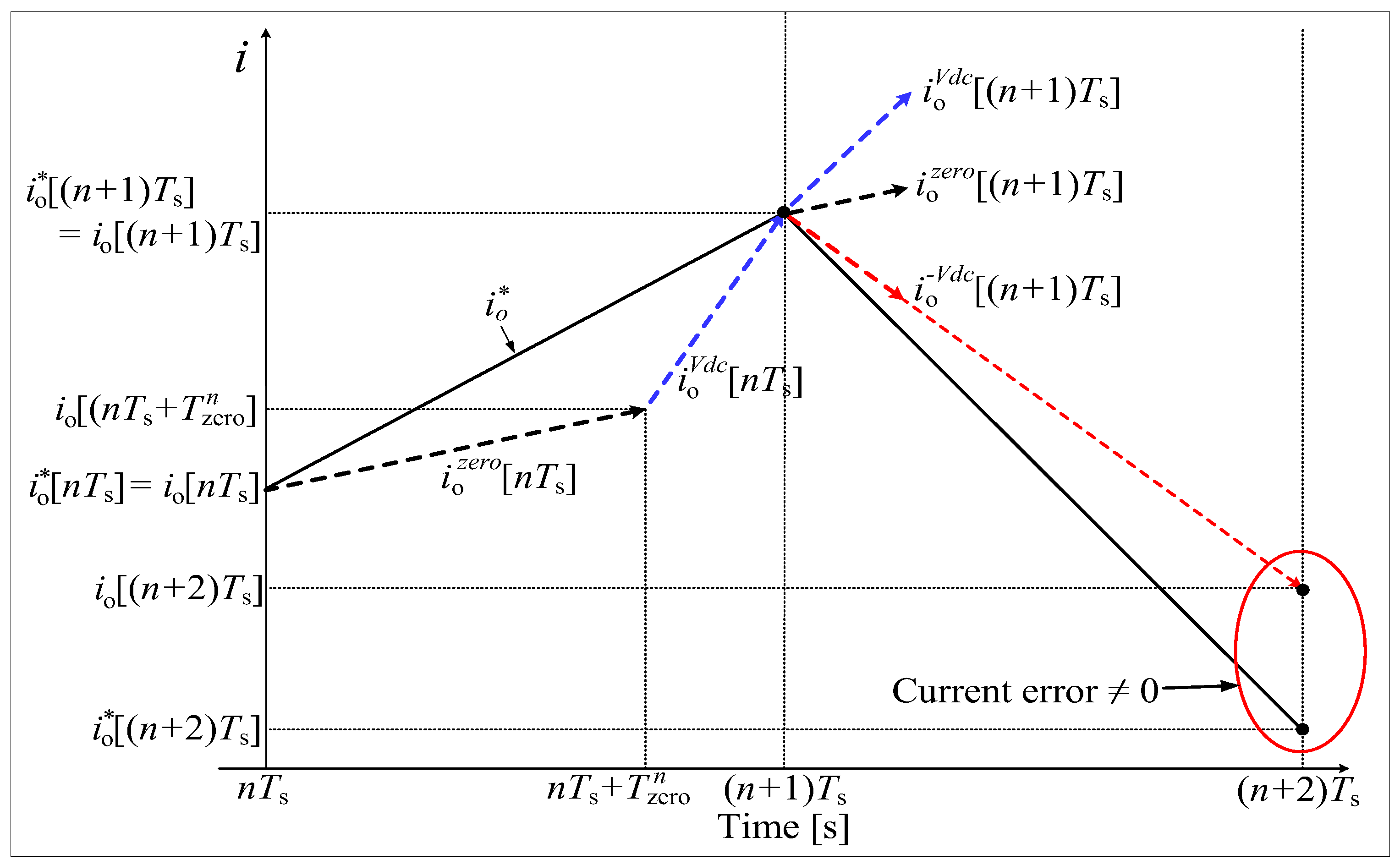
In the proposed method, the error between the reference and the actual load currents is forced to be zero at the instant of the next sampling instant at steady state. On the other hand, this current error cannot be zero during transient periods, which has a large step change in the reference current. Figure 5 shows an example of a transient state in which the slope of the reference current change during one sampling period is greater than the maximum slope of the actual current generated by one output voltage applied during the entire sampling period. As shown in Figure 5, the output voltage applied during the sampling period cannot make the current error at the (n + 2)th instant completely zero. It should be noted that the time calculated in Equation (13) does not exist between 0 and T_s. For this transient state, the proposed method sets the $T_{zero}^{n+1}$ to zero and set the time of $T_{act}^{n+1}$ to T_s to obtain a fast transient response. This allows for fast transient response using only non-zero switching states, such as the conventional predictive control, when transients occur.

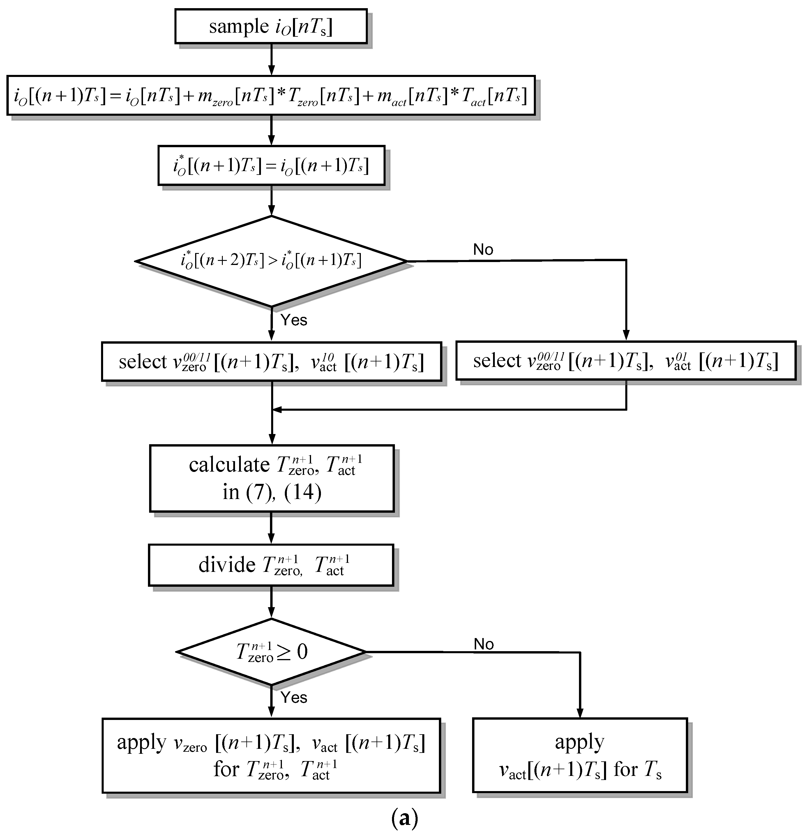
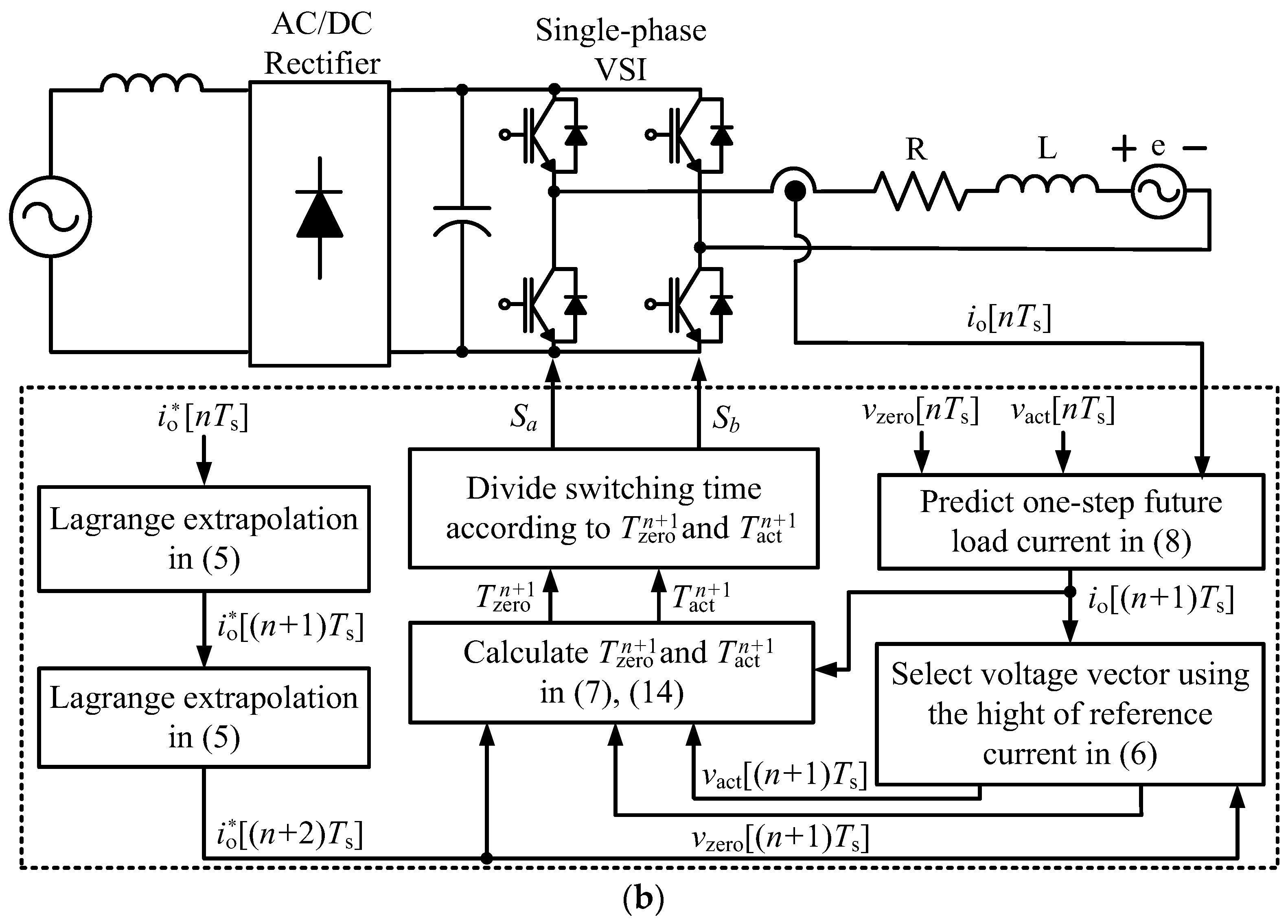
Figure 6a illustrates a flowchart to explain how the two optimal voltages are selected and how the optimal durations of the two voltages are calculated in the proposed method. In addition, a block diagram is presented in Figure 6b that includes the method by which the inevitable delay of the digital signal processor (DSP) in the practical experiment is compensated. In addition, the comparative remarks among the existing methods with a constant switching frequency and the proposed method is illustrated in

Table 1. Comparison of conventional model predictive control (MPC) methods with constant switching frequency and proposed method.

Phase	MPC Method	Vector Selection	Duty Time	PWM Block	Topology	Control Target
three-phase	Ref. [17]	Find sector like SVPWM using model-based on Vα*,Vβ*	Conventional SVPWM	Conventional SVPWM	Converter	Complex power
	Ref. [19]	Find sector like SVPWM using model-based on Vd*,Vq*	Conventional SVPWM	Conventional SVPWM	Converter	Current
	Ref. [21]	Find sector like SVPWM using model-based on Vα*,Vβ*	Conventional SVPWM	Conventional SVPWM	Inverter for PMSM	Torque and stator flux
	Ref. [22]	Find sector like SVPWM using grid angle	Zero power error at the next step	Modified SVPWM	Converter	Complex power
	Ref. [18]	Find sector like SVPWM based on V/θ using cost-function	Conventional SVPWM	Conventional SVPWM	Inverter for PMSM	Torque and stator flux
	Ref. [20]	Find sector like SVPWM using grid angle	Differentiating the cost function	Conventional SVPWM	Converter for Wind turbine	Current
single-phase	Ref. [10]	Find sector like SVPWM using model-based on Vα*,Vβ*	Conventional SVPWM	Conventional SVPWM	NPC Converter	Complex power
	Ref. [23]	Find sector like SVPWM using model-based on Vα*,Vβ*	CBPWM using modulation index		Converter	Complex power
	Proposed method	Active vector/zero vector using slope of reference current	Zero current error at next step	No PWM block	Converter	Current

.

4. Simulation and Experimental Results

Simulation of the proposed method with the single-phase VSI has been done with T_s = 200 μs, V_dc = 100 V, and an R–L load of R = 1.5 Ω and L = 24 mH. To validate the performance of the proposed method, the conv-MPC method was simulated with T_s = 33 μs, because this condition leads to almost the same average numbers of switching with the proposed method with T_s = 200 μs. Moreover, the sinusoidal PWM method along with the PI controller, which is henceforth called the PI-PWM method, was also implemented with the same carrier frequency T_c = 200 μs as the proposed method, because the proposed method results in the constant switching frequency operation, similar to the sinusoidal PWM method with the PI controller.

Table 2. Parameter values for simulation and experiment.

Parameters	Values
Vdc	100 V
R (load resistance)	1.5 Ω
L (load inductance)	24 mH
Ts (sampling period)	200 μs
Tsw (carrier period)	200 μs
favg (average switching frequency)	5 kHz
io* (reference current)	5 A

shows the parameter values for both the simulation and the experiment.

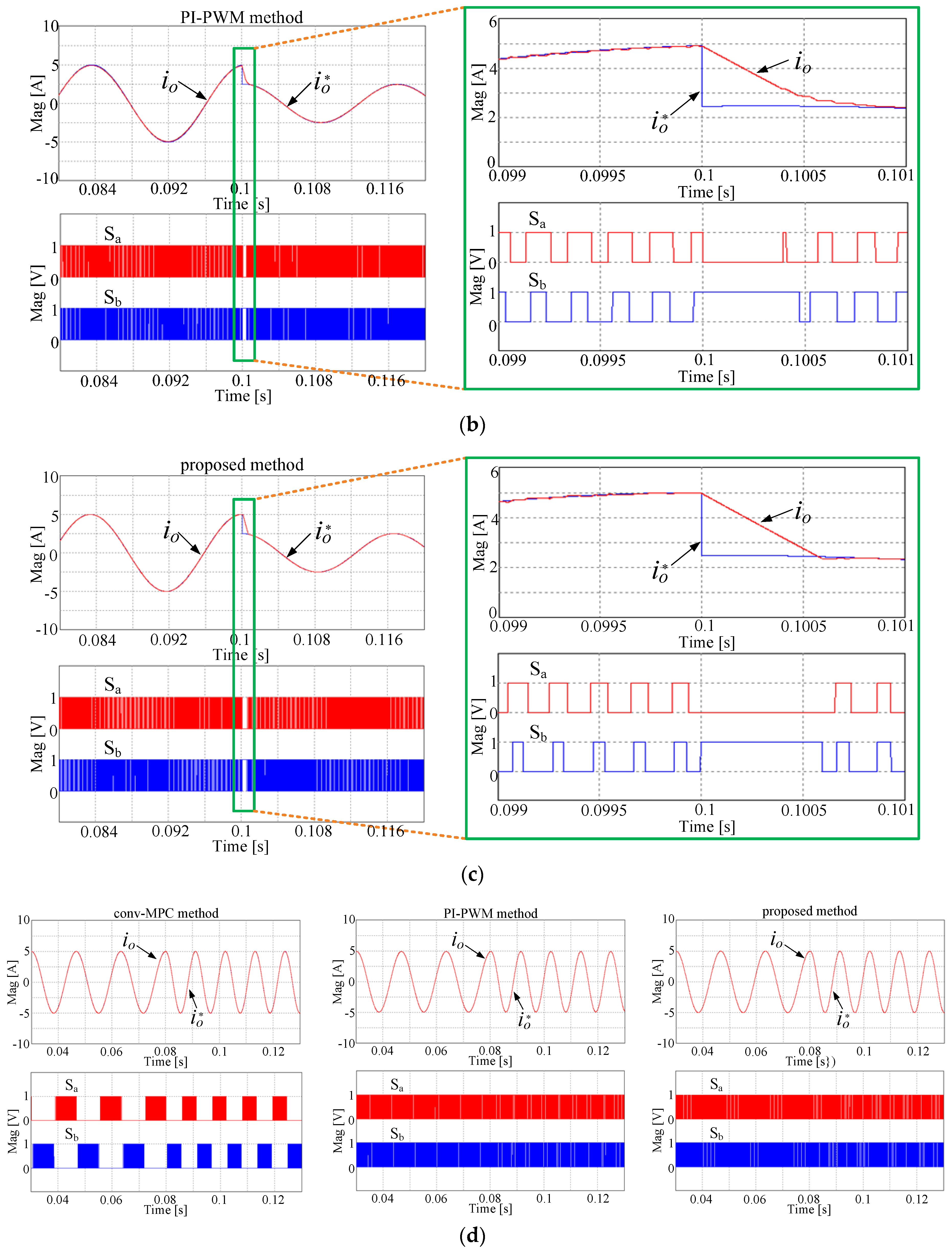
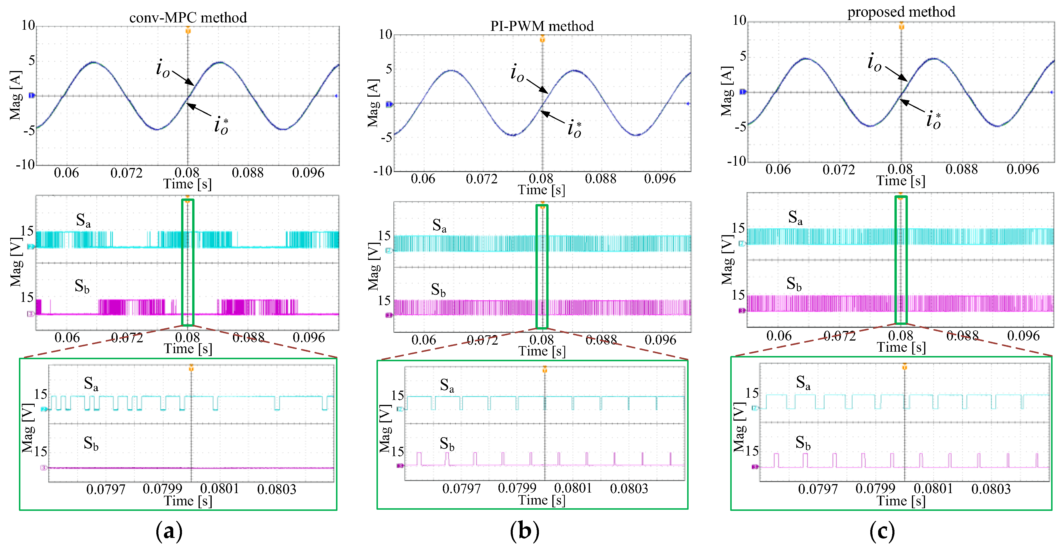
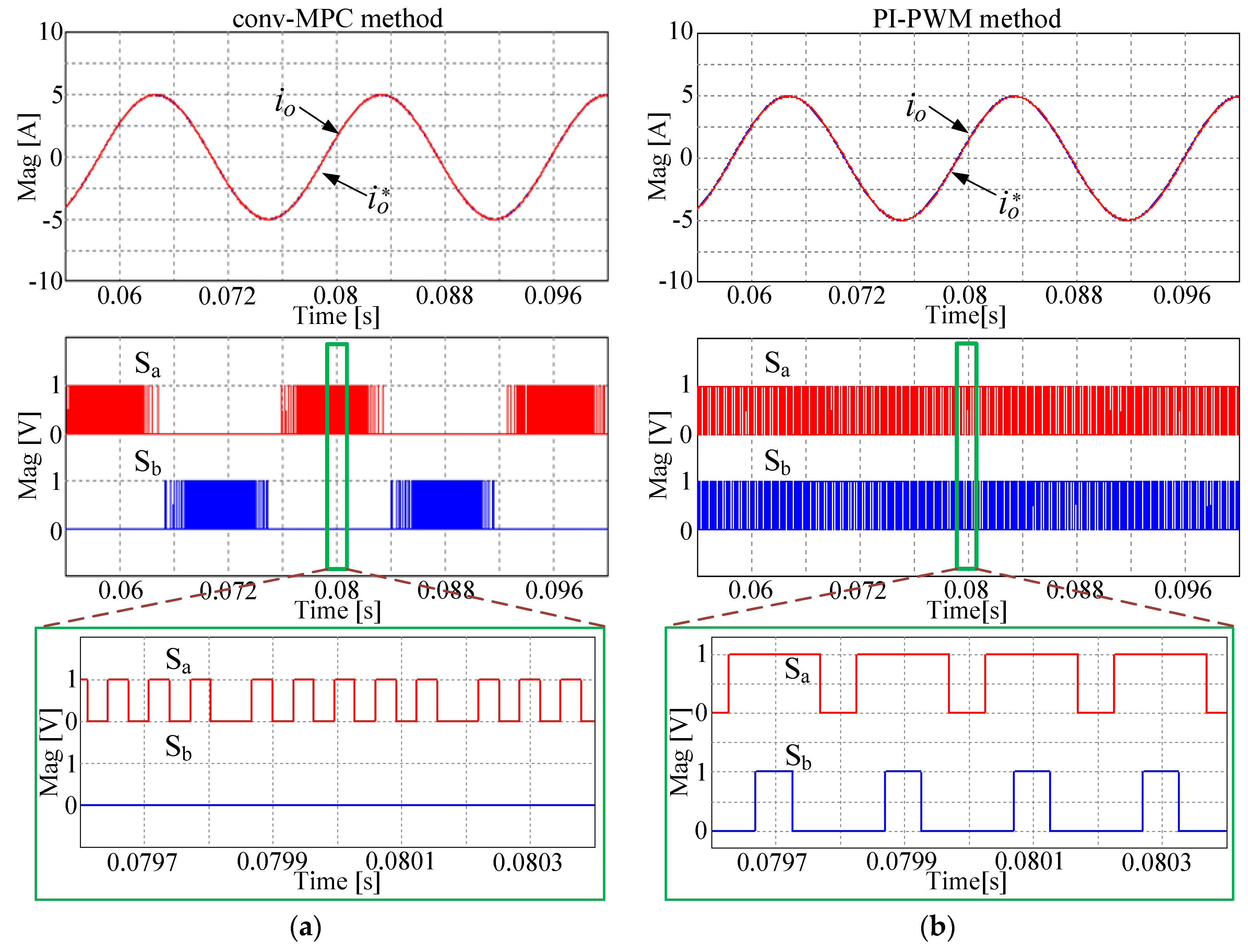
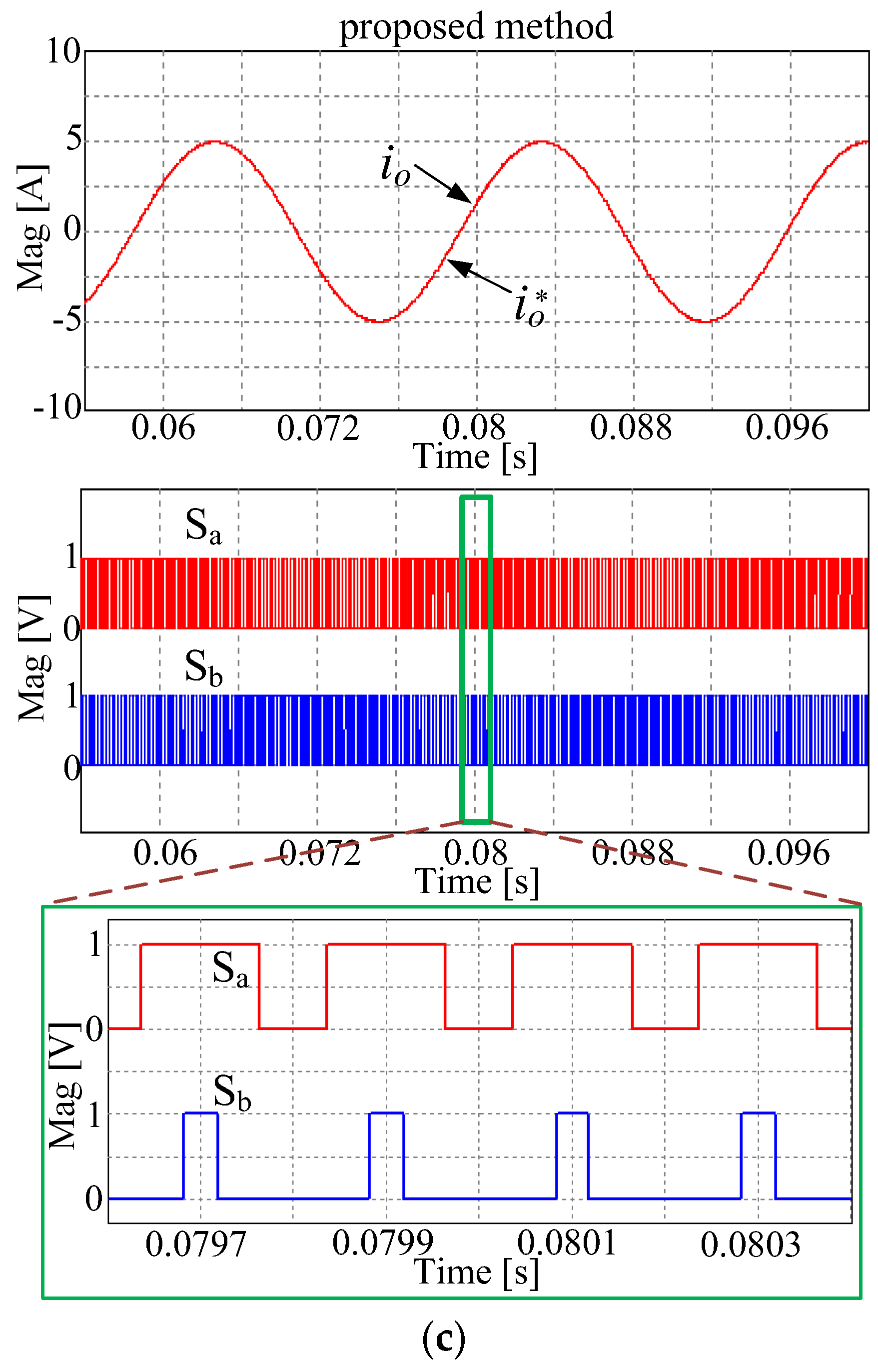
Figure 7 represents the simulation results of the output currents and the upper switch patterns during steady states in the conv-MPC, the PI-PWM method, and the proposed method. The output current waveforms obtained from the three methods show excellent regulation with the reference current, irrespective of the different algorithms. However, the patterns of the switch states (S_a, S_b) look different, where the conv-MPC method yields varying switching patterns with irregular switching waveforms. On the other hand, the switching forms of both the PI-PWM method and the proposed method are regular because both methods turn on the switches once per sampling period. 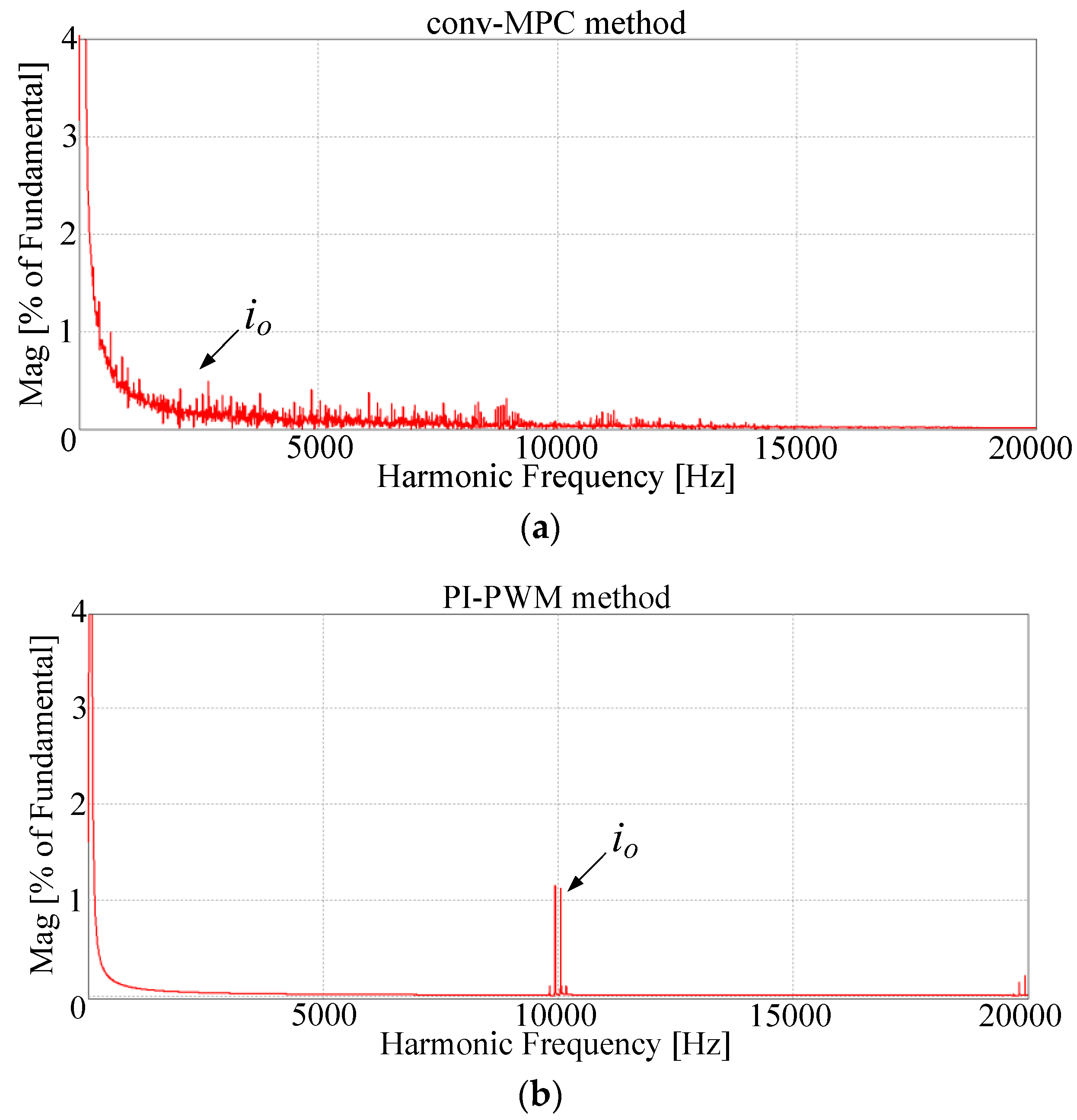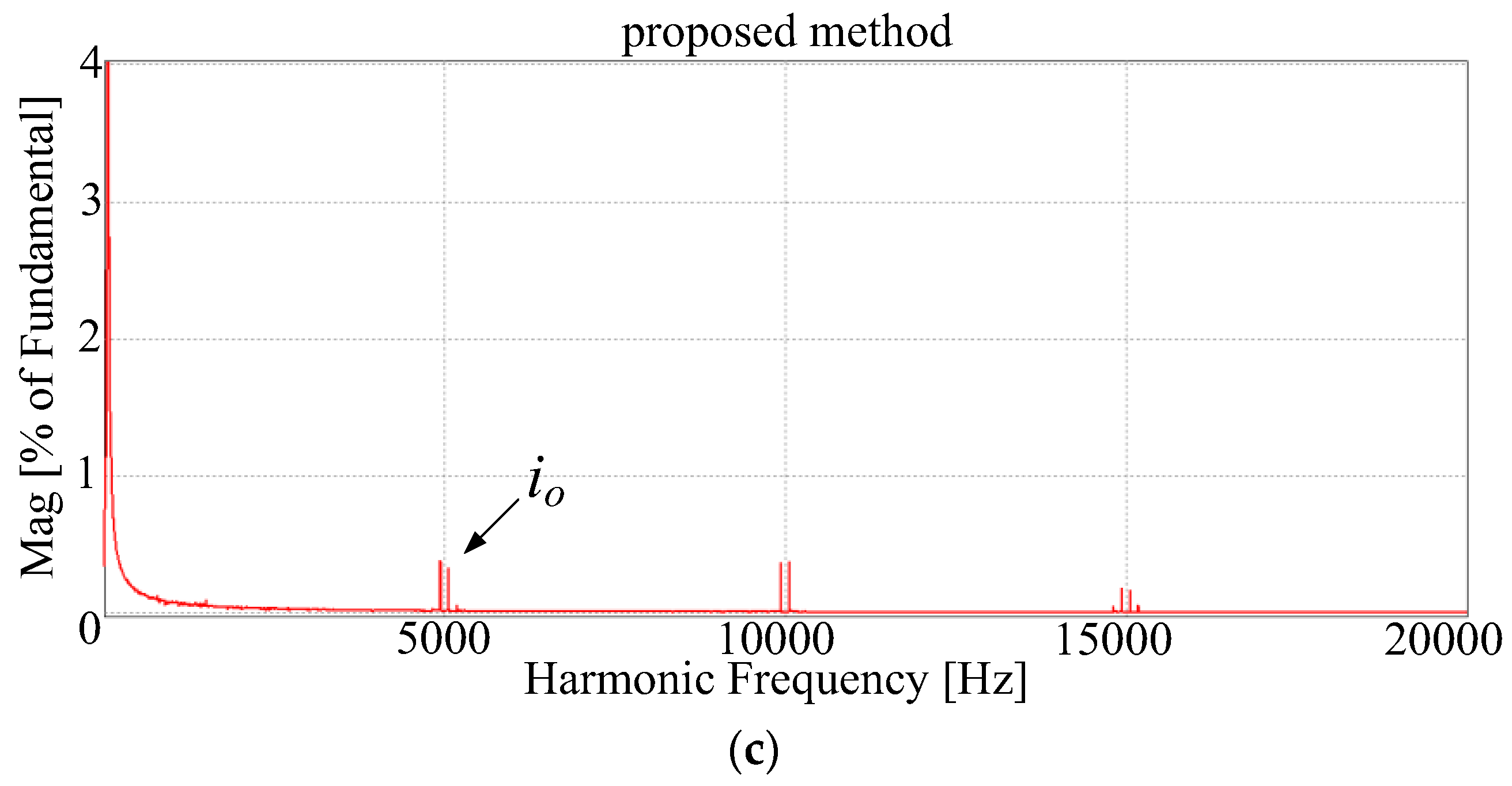This is clearly seen in Figure 8, with the FFT analysis waveforms obtained by the conv-MPC, the PI-PWM, and the proposed methods under the same average switching frequency. In contrast to the conv-MPC method with a varying frequency spectrum of output current, the proposed method results in an output current frequency spectrum concentrated in multiples of the sampling frequency, similar to the PI-PWM method, which helps design the output filter.

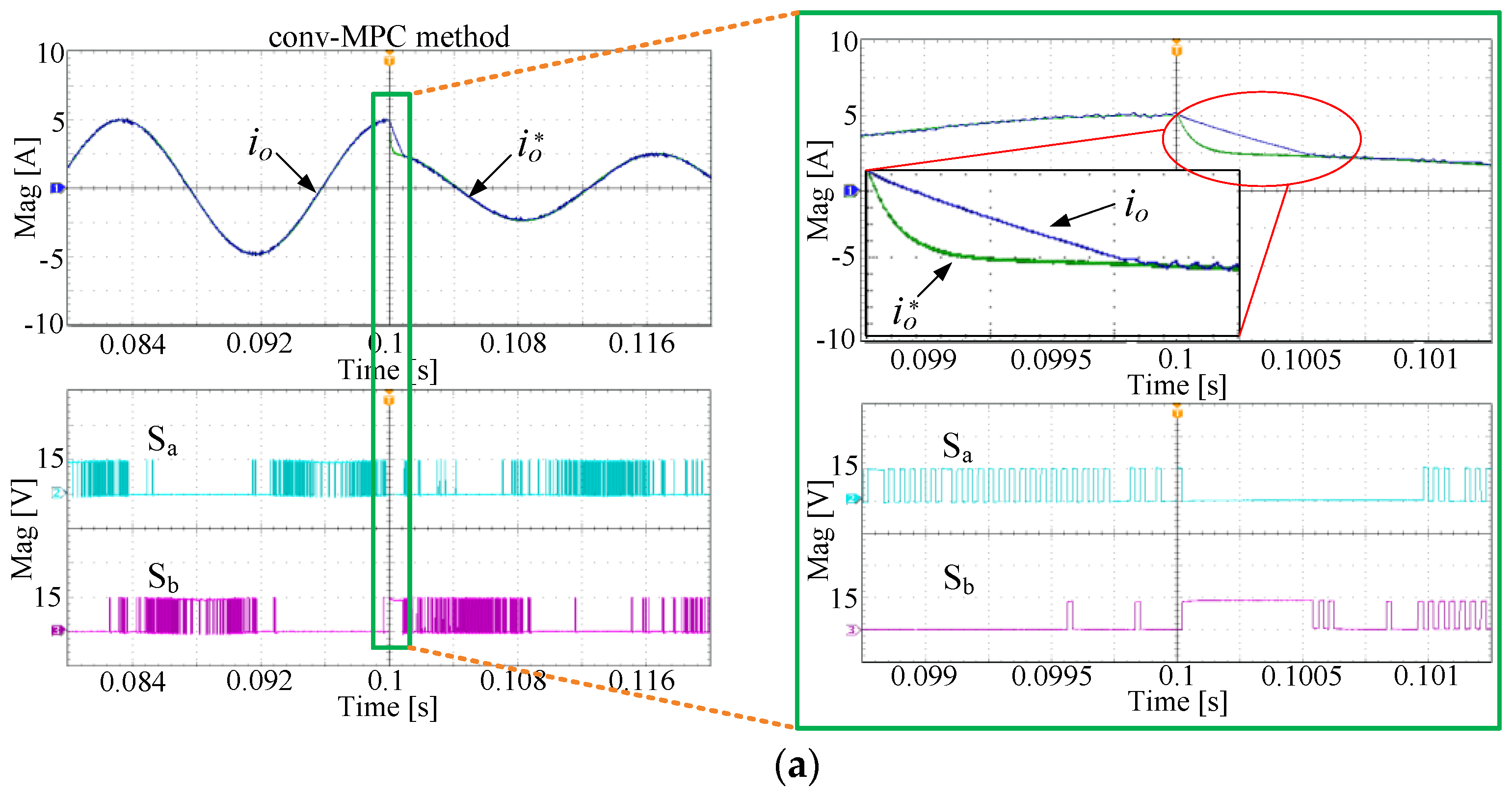
Figure 9 shows the simulation results of the output currents and the upper switching states with transient conditions and magnitude and frequency changes of the reference current. It is seen that the output current regulated by the conv-MPC method tracks the reference current with fast speed during the magnitude step change from 5 A to 2.5 A due to one switching state lasting for consecutive sampling periods. On the other hand, the PI-PWM method, which operates in both the over-modulation and the linear modulation regions, shows slower dynamics than the conv-MPC method. The proposed method utilizes one active voltage during entire sampling period like the conv-MPC method during the magnitude step- change as shown in Figure 9c, which leads to dynamics as fast as the conv-MPC method. Therefore, the proposed method can show switching patterns with fixed switching frequency like the PI-PWM method in the steady state and fast dynamic response like the conv-MPC method in the transient response. Figure 9d illustrates the transient responses of the frequency change of the three methods.

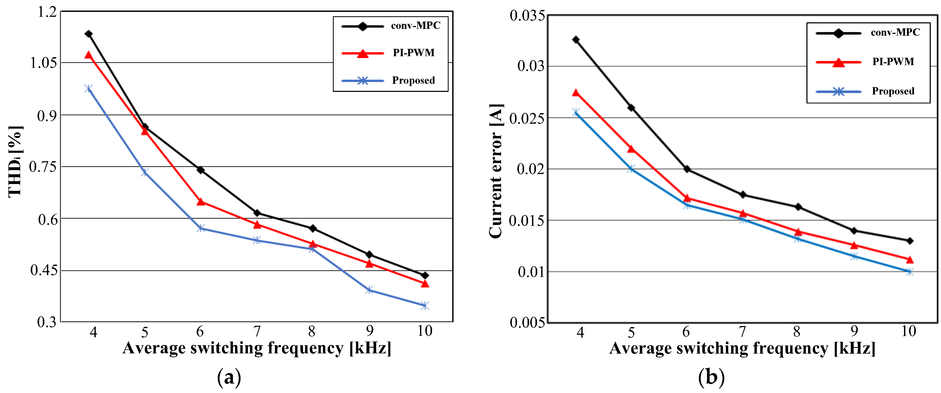
Figure 10 shows the comparative results of the conv-MPC, the PI-PWM, and the proposed methods in terms of total harmonic distortion (THD) and current errors, as a function of the switching frequency. For fair comparison, the average switching frequency of the conv-MPC method with varying switching frequency was equally set to the switching frequency of the PI-PWM and proposed methods. The total harmonic distortion (THD) and the mean absolute error values of the load currents are defined in (15) and (16).

$$THD(\%)=100\times \sqrt{\frac{i_{o2}^2+i_{o3}^2+i_{o3}^2+\cdots +i_{on}^2}{i_{o1}}}$$

(14)

$$MAE=\frac{1}{k_{samp}}{\displaystyle \sum _{n=1}^{k_{samp}}\left|i_o(n)-i_o^{*}(n)\right|},$$

(15)

where i_o1 and i_on are the fundamental and nth harmonic components in load current, respectively. The value of n is 8333 in this comparison. The value of k_samp is set to 17,000 per fundamental period. From Figure 10, it can be seen that the proposed method results in almost the same performance as the conv-MPC and the PI-PWM methods, from the perspective of the output current quality and current errors, under the conditions of the same average switching frequency. As a result, the proposed method can yield fixed switching frequency as well as the same THD and current error performance as the conv-MPC approach.

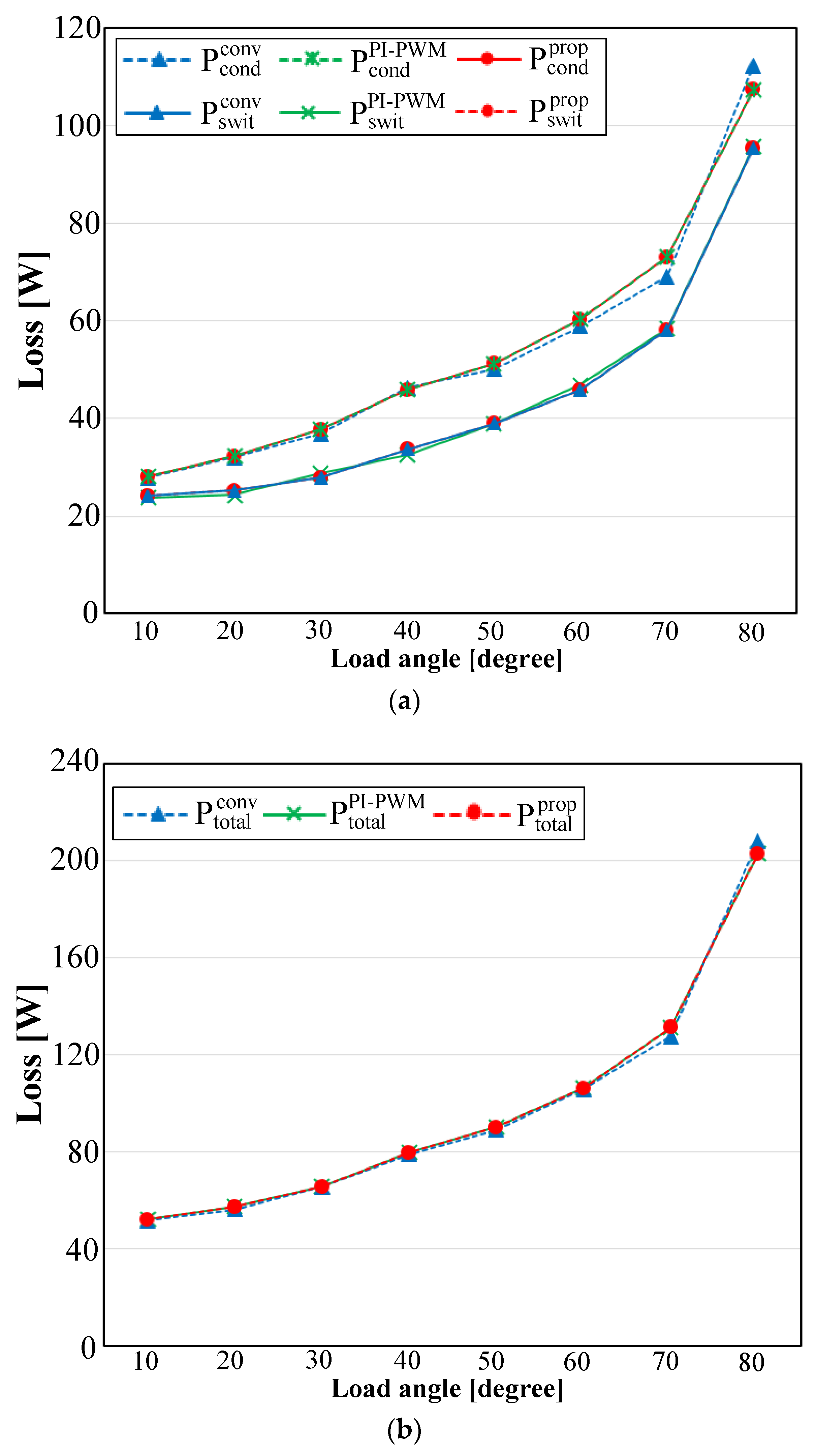
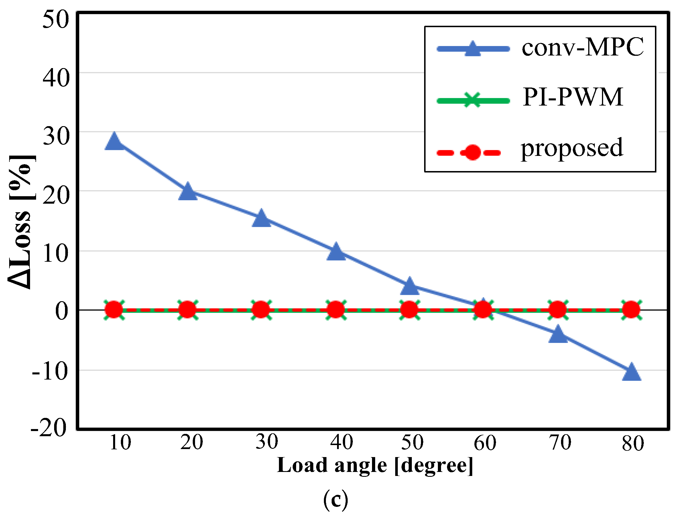
Figure 11 represents the loss performance as function of load angle under the constant power condition, where $P_{cond}^{prop}$, $P_{swit}^{prop}$, and $P_{total}^{prop}$ represents conduction loss, switching loss, and total loss of the proposed method, respectively. Likewise, $P_{cond}^{conv}$, $P_{swit}^{conv}$, and $P_{total}^{conv}$ indicate the conduction loss, switching loss, and total loss of the conventional method, respectively. The conduction loss, switching loss, and total loss of the PI-PWM method are $P_{cond}^{PI-PWM}$, $P_{swit}^{PI-PWM}$, and $P_{total}^{PI-PWM}$, respectively. With the constant power conditions, the load current increases as the load angle increases. Thus, it can be seen that both the conduction losses and the switching losses increase due to the increased load current magnitude in all three methods, as shown in Figure 11a. In addition, the switching losses of the three methods are almost equal due to the equal average switching frequency from Figure 11a. The conduction losses and the corresponding total losses of the three methods are also almost the same, as can be seen from Figure 11a,b. Although the total losses of the conv-MPC and proposed methods are similar, they have different loss distributions among the four switches. The loss imbalance between the upper and lower switches is defined by

$$\Delta Loss(\%)=100\times \frac{\left(P_{total}^{upper}-P_{total}^{lower}\right)}{P_{total}},$$

(16)

where $P_{total}^{upper}$ and $P_{total}^{lower}$ show the total loss of the upper and lower switches, respectively. Figure 11c illustrates the loss imbalance versus the load angle of the three methods. It is seen that the proposed and PI-PWM methods lead to even loss balance regardless of the load conditions, whereas the conv-MPC method shows an uneven loss profile focused on either the upper or the lower switches. Because the switching operation of the conv-MPC method happens at a certain switch, as shown in the switching waveforms in Figure 7a (only S_a), the loss profile is concentrated to either the upper or lower switch, which changes by load conditions. However, the proposed method with a regular switching operation, as shown in the switching waveforms in Figure 7c, leads to loss balance among the switching devices, just as in the PI-PWM method with the switching waveforms in Figure 7c, as shown in Figure 11c. Therefore, one can note that the proposed method exhibits the same loss performance as the PI-PWM method because of their similar switching patterns with fixed switching frequency, as shown in the switching waveforms in Figure 7b,c.

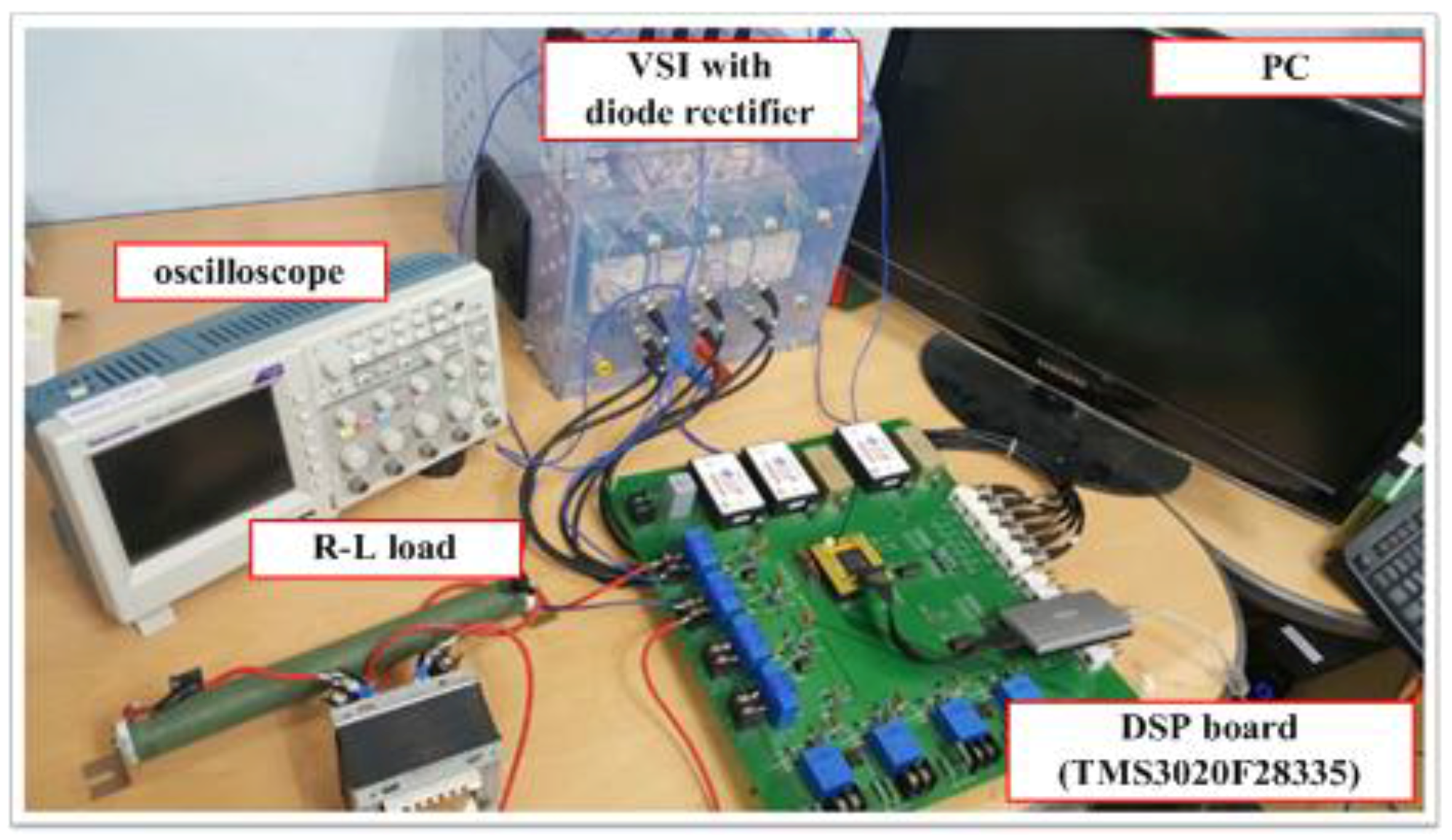
The proposed method with constant switching frequency has been validated by experimental results using a prototype setup that consists of R = 1.5 Ω, L = 24 mH, V_dc = 100 V, and T_s = 200 μs with an insulated gate bipolar mode transistor (IGBT) module (SKM50GD123D) of a single-phase voltage source inverter. For comparison, the conv-MPC method with a sampling period of 33 μs and the PI-PWM method with a switching period of T_sw = 200 μs were tested together with the proposed method. Note that the sampling frequency of the conv-MPC method was set for the purpose of obtaining the same average switching frequency as the two other methods. The three control methods were implemented on a DSP board (TMS3020F28335) to synthesize a sinusoidal output current with a 5-A magnitude and a 60-Hz fundamental frequency. 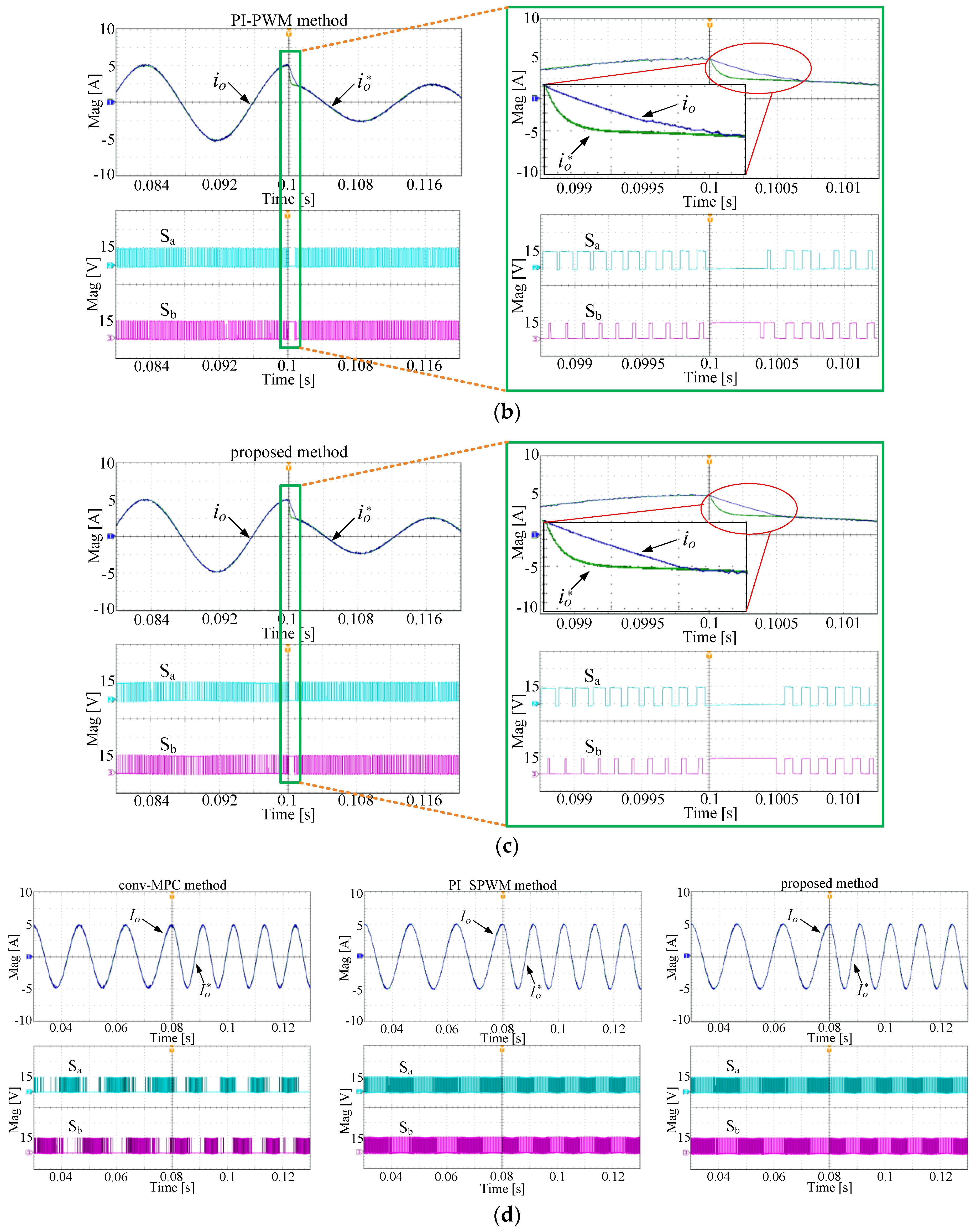A photograph of the prototype setup is shown in Figure 12.

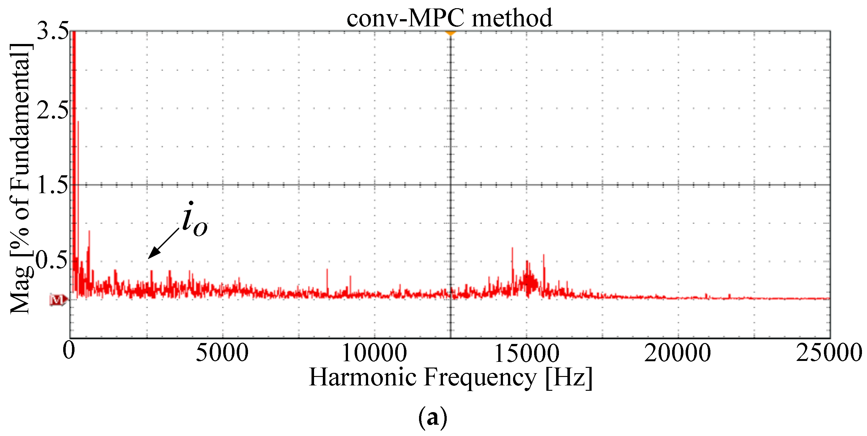
Figure 13 represents the experimental results of the output current waveform and the switching patterns of the two upper switches, obtained by the three methods. It is seen that the three methods lead to the same sinusoidal output current waveforms. However, the switching patterns of the three methods are different. Where the conv-MPC method shows switching waveforms with a variable switching frequency, the proposed method exhibits switching patterns with a constant switching frequency, which looks similar to those of the PI-PWM method.

Figure 14 illustrates the experimental performance of FFT analyses of the three methods. The conv-MPC method in Figure 14a shows the frequency spectrum spread over a wide frequency range. On the other hand, the proposed method in Figure 14b has a frequency spectrum focused on multiples of the sampling frequency, which is analogous to that of the PI-PWM method shown in Figure 14c. It is good that the switching frequency is fixed for the design of output filter, which relies on the switching frequency.

Figure 15 represents the experimental results of transient responses with magnitude and frequency step changes. The output current wave forms of the three methods track the reference changes, which are the same as the simulation results. From Figure 15, it can be seen that the dynamic response of the proposed method is as fast as the conv-MPC method. In fact, the proposed method yields a faster response than the PI-PWM method during the transient period, as shown in Figure 15b,c. Therefore, the proposed method can generate switching patterns with a constant switching frequency similar to the PI-PWM method during steady state, which facilitates the resolution of filter design issues. In addition, the proposed method can maintain dynamics as fast as those of the conv-MPC method, which is faster than the PI-PWM method.

Experimental power data were measured to calculate power losses obtained by the three control methods, where each method was performed under the same input power and load conditions. The output power of each method was measured through an oscilloscope (MSO3054). The efficiencies of the conv-MPC, the PI-PWM, and the proposed method are 94.3%, 95.5%, and 95.4%, respectively, all of which are similar, just as in the simulation study.

5. Conclusions

In this paper, an advanced predictive control algorithm with constant switching frequency for load current control is proposed for single-phase voltage source inverters. The proposed method uses only the slope of the reference current to select the switching state, and it uses the online optimization process to eliminate the error between the reference current and the actual current in the future step, thereby calculating the optimal duty cycle. This approach is simpler because the optimal switching state can be easily selected without constructing virtual orthogonal quantities, in comparison with existing studies of single-phase converters. In addition, the proposed method develops switching patterns with a fixed switching frequency by appropriately dividing the zero-voltage state and the non-zero-voltage state, without employing the PWM modules. The proposed method has advantages of simple optimal voltage selection and not using PWM block, compared to existing methods. The performance of the proposed method was compared with that of the conventional predictive current control method with varying switching frequency and that of the PI-controller-based PWM method. The proposed method can generate switching patterns with a constant switching frequency, similar to the PI-controller-based PWM method during steady state, which facilitates the resolution of filter design issues. In addition, the proposed method can maintain the fast dynamics of the conventional predictive current control method, which is faster than the PI-controller-based PWM method. The performance of the proposed method was validated with both simulation and experimental results for single-phase voltage source inverters.